How Much Does the Dynamic F0 Curve Affect the Expression of Emotion in Utterances?

Abstract

The modulation of vocal elements, such as pitch, loudness, and duration, plays a crucial role in conveying both linguistic information and the speaker’s emotional state. While acoustic features like fundamental frequency (F0) variability have been widely studied in emotional speech analysis, accurately classifying emotion remains challenging due to the complex and dynamic nature of vocal expressions. Traditional analytical methods often oversimplify these dynamics, potentially overlooking intricate patterns indicative of specific emotions. This study examines the influences of emotion and temporal variation on dynamic F0 contours in the analytical framework, utilizing a dataset valuable for its diverse emotional expressions. However, the analysis is constrained by the limited variety of sentences employed, which may affect the generalizability of the findings to broader linguistic contexts. We utilized the Ryerson Audio-Visual Database of Emotional Speech and Song (RAVDESS), focusing on eight distinct emotional states performed by 24 professional actors. Sonorant segments were extracted, and F0 measurements were converted into semitones relative to a 100 Hz baseline to standardize pitch variations. By employing Generalized Additive Mixed Models (GAMMs), we modeled non-linear trajectories of F0 contours over time, accounting for fixed effects (emotions) and random effects (individual speaker variability). Our analysis revealed that incorporating emotion-specific, non-linear time effects and individual speaker differences significantly improved the model’s explanatory power, ultimately explaining up to 66.5% of the variance in the F0. The inclusion of random smooths for time within speakers captured individual temporal modulation patterns, providing a more accurate representation of emotional speech dynamics. The results demonstrate that dynamic modeling of F0 contours using GAMMs enhances the accuracy of emotion classification in speech. This approach captures the nuanced pitch patterns associated with different emotions and accounts for individual variability among speakers. The findings contribute to a deeper understanding of the vocal expression of emotions and offer valuable insights for advancing speech emotion recognition systems.

1. Introduction

The modulation of vocal elements, such as pitch, loudness, duration, and voice quality, across syllables in an utterance conveys both linguistic information—such as prominence and prosodic phrasing—and non-linguistic information, notably the speaker’s emotional state [1]. Emotional states are psychological conditions indicated by neurophysiological changes, being typically associated with thoughts, feelings, and behavioral responses [2]. These states are communicated not only through facial expressions but also through vocal expressions in both linguistic and paralinguistic contexts [3].

When speaking, individuals inherently transmit their emotional status alongside linguistic content. Two prevailing theories attempt to explain how emotions influence behavior and expression: the dimensional theory and the discrete emotion theory [4]. The dimensional theory, proposed by [5] and further developed by [6], suggests that emotions can be distinguished along two primary dimensions: valence (the positivity or negativity of the emotion) and arousal (the intensity of the emotion). According to this perspective, basic emotions are defined within this two-dimensional emotional space.

In contrast, the discrete emotion theory, initially devised by [7] and extensively developed by [2], posits that there are specific biologically and neurologically distinct basic emotions. Ekman’s research supports the view that emotions are discrete, measurable, and physiologically distinct, and certain emotions are universally recognized across cultures. These basic discrete emotions typically include happiness, sadness, anger, fear, disgust, and surprise.

Acoustic features play a critical role in the analysis and recognition of emotional speech [4,8]. Features such as the fundamental frequency (F0), variability (pitch), voice intensity (energy), and Mel-Frequency Cepstral Coefficients (MFCCs) are commonly used in automatic emotion recognition tasks. MFCCs capture the human auditory frequency response and represent the signal more effectively than raw frequency bands [9,10,11]. However, some studies have reported poor emotion classification results using MFCCs, possibly due to the embedded pitch filtering during cepstral analysis that may obscure important pitch-related emotional cues [8].

Despite the availability of rich acoustic data, challenges remain in accurately classifying emotions based on speech. This is partly due to the complexity of emotional expression and the limitations of analytical methods that often simplify dynamic vocal data, potentially overlooking intricate patterns indicative of specific emotions [12]. For instance, previous research suggests that some acoustic features are associated with general characteristics of emotion rather than specific emotional states, supporting the idea that grouping emotions by activation levels (e.g., high-activation emotions like anger and joy) can improve recognition performance [13,14]. However, distinguishing between emotions within similar activation levels remains challenging.

Intonation, particularly pitch contour patterns, has been recognized as important for expressing emotional states [15,16,17,18,19]. Previous works [15,16,17,18,19] have made significant contributions to enhancing our understanding of the role of F0 in emotional speech. However, previous studies often used simplistic intonation parameters, which may contribute to lower classification rates of emotional types based on acoustic features [8]. Simplifying dynamic data can reduce the data size and make traditional statistical methods easier to apply, but it may also lead to the loss of potentially interesting patterns [20]. Some studies, such as [15,19], have modeled F0 dynamics in emotional speech. But the previous approaches had a limitation in allowing us to evaluate not only the general trends of F0 contours but also their interaction with speaker-specific variability and temporal effects.

To address these challenges, more sophisticated statistical techniques are needed, particularly those capable of identifying non-linear patterns in dynamic speech data. Generalized Additive Mixed Models (GAMMs) offer such capabilities, allowing for the modeling of non-linear trajectories and interactions [21]. While several speech emotion recognition frameworks combine different feature types, the direct incorporation of dynamic F0 contours into emotion classification systems using GAMMs has not been extensively explored [8].

This study aims to classify emotional states by extracting and analyzing dynamic F0 contours using GAMMs, which have proven effective in capturing non-linear trajectory patterns in speech data [22,23]. By leveraging GAMMs, we seek to uncover the underlying patterns of vocal expression associated with different emotional states, thereby refining emotion classification in speech and advancing our understanding of the vocal expression of emotions.

To achieve this, a dataset with classified emotion types is necessary. Additionally, the results of modeling based on the F0 curve should be compared to the state of the art achieved using the same data to assess the level of explanatory power. For reasons like this, the RAVDESS dataset was chosen. The RAVDESS dataset consists of only two sentences per emotion, which imposes certain limitations on the generalizability of the findings from this study. While the dataset is valuable for controlled experimentation, the limited number of sentences may not capture the full variability present in natural speech, thereby restricting the extent to which these results can be applied to broader contexts. Nevertheless, the dataset has a few strengths: Professional actors and controlled recording conditions ensure consistent audio quality. The dataset covers a wide range of emotions, which is essential for comprehensive emotion classification. Equal numbers of male and female actors facilitate gender-related analyses. Using the same sentences across emotions and actors controls for linguistic variability, allowing us to focus on acoustic features related to emotion.

Prior Classification Accuracy Using the RAVDESS Dataset

Several prior studies have attempted emotion classification using the RAVDESS dataset with varying degrees of success. For instance, Ref. [24] utilized Support Vector Machines (SVMs) with features selected via Continuous Wavelet Transform (CWT) and achieved an accuracy of 60.1%. Additionally, Ref. [25] focused on a subset of four emotions and obtained an accuracy of 57.14% using group multi-task feature selection.

Deep learning approaches have reported higher accuracies. For example, Ref. [26] implemented a Deep Neural Network (DNN) using spectrograms and achieved a 65.9% accuracy. Also, Ref. [27] fine-tuned a pre-existing DNN and, using VGG-16, reported an accuracy of 71%. Similarly, Ref. [28] employed a one-dimensional deep CNN with a combination of acoustic features like MFCCs, mel-scaled spectrograms, chromograms, spectral contrast features, and tonnetz (e.g., tone network) representations, reaching an accuracy of 71.61%.

While these deep learning models outperform the human accuracy rates of 67% reported by [29], they often function as black boxes, offering limited insight into which features drive the classification. The use of multiple acoustic features in these models combines various sound characteristics, potentially leading to improved performance. However, this complexity makes it challenging to discern the contribution of individual features to the overall classification, which can hinder the interpretability and explainability of the results.

Our approach offers the following contributions: First, we utilize the full temporal dynamics of F0 contours rather than static or simplified representations, capturing intricate pitch patterns associated with specific emotions. Second, we apply GAMMs to model non-linear relationships and individual variability in emotional speech, accommodating the complex interplay between time, emotion, and speaker characteristics. Finally, by integrating dynamic F0 contours with GAMMs, we aim to improve accuracy of emotion classification, particularly for emotions with similar activation levels.

The remainder of this paper is organized as follows: In Section 2, we present our methodology, including data collection, preprocessing, and the GAMM approach. Section 3 details the results of our analysis and compares them with those of previous approaches. In Section 4, we discuss the implications of our findings and potential limitations. Finally, in Section 5, we draw conclusions and indicate possible directions for future research.

2. Materials and Methods

2.1. Materials

For the statistical modeling of emotion classification, we employed the Ryerson Audio-Visual Database of Emotional Speech and Song (RAVDESS) [29], a validated multimodal dataset widely used in emotion recognition research. The RAVDESS dataset comprises 2880 audio–visual files, including both speech and song modalities, expressed across a range of emotions.

For our analysis, we selected the audio-only speech files (modality code 03, vocal channel 01), focusing on the emotional expressions relevant to our study. Each actor contributed 60 recordings, resulting in a total of 1440 audio files. This selection ensured a balanced representation of genders and emotions, providing a robust dataset for statistical modeling. These files feature 24 professional actors (12 female and 12 male), each vocalizing two semantically neutral sentences: (1) “Kids are talking by the door.” (2) “Dogs are sitting by the door.”

Each sentence is articulated with varying emotional expressions and intensities, except for the neutral emotion, which is presented only at a normal intensity.

Emotional Categories and Data Organization

The RAVDESS dataset encompasses eight distinct emotional states: (1) neutral, (2) calm, (3) happy, (4) sad, (5) angry, (6) fearful, (7) disgust, and (8) surprise. Each emotion (except neutral) is expressed at two levels of intensity: normal and strong. Every actor provides two repetitions of each sentence per emotional expression and intensity level, resulting in a comprehensive set of emotional speech data.

To streamline data access and analysis, we reorganized the audio files from their original actor-specific directories into eight consolidated folders, each corresponding to one of the emotional categories. This reclassification facilitated efficient retrieval and processing of the data associated with each emotion.

Each audio file in the RAVDESS dataset is uniquely named following a structured convention that encodes metadata about the recording. The file-naming convention consists of a seven-part numerical identifier in the format Modality-VocalChannel-Emotion-EmotionalIntensity-Statement-Repetition-Actor.

Table 1. Meta information and identifiers used in the RAVDESS (Ryerson Audio-Visual Database of Emotional Speech and Song) dataset.

	Meta Information	Identifiers
1	Modality	01 = full AV; 02 = video only; 03 = audio only
2	Vocal Channel	01 = speech; 02 = song
3	Emotion	01 = neutral; 02 = calm; 03 = happy; 04 = sad; 05 = angry; 06 = fearful; 07 = disgust; 08 = surprise
4	Emotional Intensity	01 = normal; 02 = strong (cf. no strong intensity for the “neutral” emotion)
5	Statement	01 = “Kids are talking by the door”; 02 = “Dogs are sitting by the door”
6	Repetition	01 = 1st repetition; 02 = 2nd repetition
7	Actor	01 to 24 (24 actors)
8	Gender	Odd-numbered actors = male; even-numbered actors = female

summarizes the identifiers used in the RAVDESS dataset. This naming convention facilitated systematic organization and the retrieval of files based on attributes such as emotion, intensity, and actor identity.

2.2. Methods

2.2.1. Preprocessing of F0 Contours

To enhance the accuracy of emotion classification in speech, we focused on the sonorant segments of utterances, where fundamental frequency (F0) extraction is the most reliable. F0 values were converted into semitones relative to a standard 100 Hz baseline to normalize inherent pitch variances across speakers.

We utilized the Ryerson Audio-Visual Database of Emotional Speech and Song (RAVDESS) dataset [29], which comprises 1440 audio files representing a range of emotions portrayed by professional actors. Forced alignment techniques synchronized the textual scripts with their corresponding audio recordings. This alignment was facilitated using Python libraries such as Parselmouth [30], librosa [11,31], and tgt [32], which collectively enabled the processing of audio files and the extraction of vocal features like vowel duration and F0 variability, which are essential for nuanced emotion classification.

2.2.2. Pitch Extraction and Processing

Pitch extraction was conducted using the autocorrelation method via Praat [33], interfaced through Parselmouth. A pitch ceiling of 450 Hz was set to ensure data fidelity and to accommodate the pitch range of the speakers. The extracted F0 values were smoothed to remove non-numerical anomalies, thereby preserving the integrity of the dataset for analysis.

Our dataset comprised over 126,000 measurement points obtained from 1440 speech trials, with an average word duration of approximately 0.78 s. Due to the fixed sampling rate and variations in word lengths, the number of sample points per word varied, averaging about 78 measurements per word. To address this variability and maintain consistency across the dataset, we employed the resampy package (v.0.4.2) [34] to interpolate the F0 data. This interpolation adjusted the resampled files to match the maximum utterance length in the dataset while retaining the essential shape of the pitch contours. This process was crucial for ensuring that the statistical modeling would be comparable across utterances of different durations.

Our analysis concentrated on sonorant segments, particularly vowels, where F0 can be accurately extracted. We noted that adjacent obstruents and sonorants could exhibit subtle effects on the F0, which warranted careful attention. By converting F0 values to semitones relative to a 100 Hz reference tone, we standardized the units for comparison and analysis across different speakers and recordings.

All RAVDESS speech files were subjected to precise time alignment using forced alignment techniques. This process allowed us to focus our analysis on both durational and segmental features, deepening our understanding of the complexities of emotional speech. Recognizing that accurate emotion classification requires a multitude of features, we ensured that our dataset was rich in relevant vocal characteristics.

Figure 1 illustrates an example of the F0 values in semitones extracted from a sample audio file (“03-01-08-01-01-01-03.wav”). The left panel shows the original F0 values, while the right panel demonstrates the resampled pitch contours using the resampy function. In the right panel, the original pitch values are represented by a solid line, and the resampled pitch values are depicted by a dotted line. This visualization highlights the effectiveness of our resampling technique in preserving the inherent shape of the pitch contours, providing a robust foundation for subsequent statistical modeling.

2.3. GAMM

To capture the complex, non-linear relationships inherent in emotional speech data, we employed Generalized Additive Mixed Models (GAMMs). A Generalized Additive Mixed Model (GAMM) is an extension of the generalized linear mixed model (GLMM) that incorporates non-linear relationships in the data through smooth functions. GAMMs are adept at revealing complex patterns that are not apparent under linear analysis, making them particularly powerful for nuanced analyses where relationships between variables are not strictly linear or change across different levels of another variable. The basic formula for a Generalized Additive Mixed Model (GAMM) can be expressed as follows:

$$y=\beta 0+{\displaystyle \sum }_j{s}_j\left(x_j\right)+{\displaystyle \sum }_k{b}_k{z}_k+ϵ$$

in which ${\beta }_0$ is the intercept term, and the term $\sum _j{s}_j\left(x_j\right)$ represents the sum of smooth functions $f_j$ applied to predictor variable $x_j$. The term $\sum _k{b}_k{z}_k$ is for the sum of random effects $b_k$ for grouping variables $z_k$, capturing variability in $y$ due to random factors. $ϵ$ indicates the error term. In summary, the GAMM combined fixed effects and random effects to model complex data with both non-linear patterns and hierarchical measures [19,20].

In our study, we embraced the flexibility of GAMMs to interpret the intricate dynamics within our emotional speech dataset. We constructed our GAMMs using the mgcv package in R (version 1.8-36) [21], a robust environment for statistical computing and graphics. The mgcv package offers comprehensive tools for building and evaluating GAMMs, facilitating the modeling of complex data structures and relationships. It enables the modeling of complex, non-linear, and non-fixed relationships between predictors and the response variable: in our case, the various speech features influencing emotional expression. The visualization and interpretation of the models were enhanced using the itsadug package (version 2.4) in R [35], which provides utilities for plotting smooths, assessing model diagnostics, and interpreting interaction effects. This combination allowed us to effectively communicate the subtleties and strengths of our models through graphical representations.

The use of GAMMs in phonetic research is well established, with studies demonstrating their efficacy in analyzing dynamic speech patterns [36,37,38,39,40]: Ref. [36] applied GAMMs to investigate phonetic variations and changes in Scottish English, capturing complex interactions between social factors and speech acoustics. Ref. [37] utilized GAMMs to analyze articulatory trajectories in tongue movement data, revealing non-linear patterns associated with language proficiency. Ref. [38] employed GAMMs to model the time-varying nature of electrophysiological responses in psycholinguistic experiments, showcasing the models’ capacity to handle time-series data.

These precedents highlight the suitability of GAMMs for our study, which involves modeling the non-linear F0 contours associated with different emotional expressions over time. GAMMs have also been instrumental in investigating the temporal dynamics of speech and the interplay between articulatory movements and acoustic outcomes [22,23,32], further evidencing their utility in phonetics.

Model Specification

By leveraging this advanced statistical approach, our objective is to uncover the underlying patterns of vocal expression associated with different emotional states, elucidating how these patterns may vary across different speakers or linguistic contexts. Through the rigorous application and interpretation of GAMMs, we aim to contribute significantly to the growing body of knowledge in emotional speech processing and phonetic analysis, providing insights that can be applied across various fields, including speech technology, clinical diagnostics, and communication studies.

The comprehensive approach we have adopted, encompassing sophisticated statistical modeling and careful visualization, is designed to offer a more nuanced understanding of the complex relationship between speech features and emotional expression. The results of our GAMM analysis promise to provide a rich, multi-dimensional perspective on the phonetic underpinnings of emotional speech, potentially informing both theoretical frameworks and practical applications in speech science.

3. Results

We developed a series of Generalized Additive Mixed Models (GAMMs) to classify the eight emotion labels in the RAVDESS dataset based on fundamental frequency (F0) contours. Our modeling approach progressively incorporated additional complexity to better capture the nuances of emotional speech.

3.1. Baseline Model

The first model (Model 0) was designed to estimate the average (constant) F0 across utterances among the eight emotion labels. We used the bam (Big Additive Model) function from the mgcv package in R [21] to fit the Generalized Additive Model (GAM). The bam function is specifically optimized for large datasets and complex models, making it suitable for our dataset comprising over 750,000 observations. In contrast, the alternative gam function can become prohibitively slow for complex models when fitted to datasets exceeding 10,000 data points, thus reinforcing our choice of bam for efficient computation. The formula for Model 0 can be interpreted as follows:

$$Model 0: F0=\beta 0+{\sum }_{i=1}^8{\beta }_i·Emotio{n}_i+ϵ$$

In this case, the inclusion of a single predictor, emotions, allows the model to estimate a constant difference among its eight levels. The parametric coefficients for Model 0 are presented in

Table 2. Parametric coefficients of Model 0. The table includes the estimates, standard errors, t-values, and p-values for the intercept and each emotional category (neutral set as intercept, calm, sad, fear, angry, happy, disgust, and surprise).

	Estimate	Std. Error	t Value	Pr (>|t|)
(Intercept)	7.8841	0.0313	252.3	<2 × 10−16	*** 1
Calm	−0.6751	0.0383	−17.6	<2 × 10−16	***
Sad	2.8221	0.038	73.7	<2 × 10−16	***
Fear	7.3384	0.0383	191.7	<2 × 10−16	***
Angry	6.9627	0.0383	181.9	<2 × 10−16	***
Happy	5.7407	0.0383	150.0	<2 × 10−16	***
Disgust	2.2176	0.0383	57.9	<2 × 10−16	***
Surprise	6.2874	0.0383	164.3	<2 × 10−16	***

¹ Significance codes used throughout the table: 0, ‘***’; 0.001, ‘**’; 0.01, ‘*’; 0.05, ‘.’; 0.1, ‘ ’ 1.

. Note that the standard errors are identical for all emotion categories except for the intercept. Each emotion is treated as a fixed effect, and the model estimates a single, pooled error term that applies across all levels of the factor. Thus, the model’s residual error is shared across all categories, resulting in the same standard error.

Table 3. Summary statistics for Model 0.

R-sq. (adj)	Deviance Explained	fREML	Scale est.	N
0.145	14.5%	2.5511 × 106	49.317	757,440

provides the key summary statistics for Model 0, providing a clear overview of the model’s performance and fit to the dataset. The adjusted R-squared value is 0.145, suggesting that 14.5% of the variance in the response variable is explained by the model. The restricted maximum likelihood (REML) estimate is 2.5511 × 10⁶, and the estimated scale parameter is 49.317. The model was fitted to a dataset comprising 757,440 observations.

Figure 2 illustrates the distribution of the mean F0 for each emotion. It is evident in the figure that the mean F0 alone is not sufficient in explaining the types of emotion.

3.2. Incorporating Non-Linear Time Effects

We fit another simple model (Model 1) that includes the constant difference among emotions but only a single smooth. The function s sets up a smooth over the parameter (i.e., time). As such, Model 1 assumes that the pattern over time is the same for all the eight emotions. The modified Generalized Additive Model was specified to include a non-linear pattern over time. In this model, the Helmert contrast was applied with the order of neutral, calm, sad, fear, angry, happy, disgust, and surprise (the same order that is observed in Figure 3).

$$Model1:F0=\beta 0+{\displaystyle \sum }_{i=1}^8{\beta }_i·Emotio{n}_i+s\left(Time\right)+ϵ$$

The output of Model 1 is given in

Table 4. Parametric coefficients of Model 1.

	Estimate	Std. Error	t Value	Pr (>|t|)
(Intercept)	7.8841	0.0304	259.3	<2 × 10−16	***
Calm	−0.675	0.0372	−18.1	<2 × 10−16	***
Sad	2.8221	0.0372	75.9	<2 × 10−16	***
Fear	7.3384	0.0372	197.3	<2 × 10−16	***
Angry	6.9627	0.0372	187.2	<2 × 10−16	***
Happy	5.7407	0.0372	154.3	<2 × 10−16	***
Disgust	2.2176	0.0372	59.6	<2 × 10−16	***
Surprise	6.2874	0.0372	169.0	<2 × 10−16	***

for coefficient estimates and

Table 5. Approximate significance of smooth terms.

Title 1	edf	Ref.df	F	p-Value
s(Time)	8.96	9	4945	<2 × 10−16 ***

for the approximate significance of smooth terms:

The intercept represents the estimated mean F0 for the neutral emotion at the reference time point. The coefficients for each emotion indicate the difference in mean F0 compared to the neutral emotion, controlling for the effect of time. The standard errors for each emotion remain identical because the categorical variable is still treated as a fixed effect without interaction with time.

The approximate significance of the smooth term s(Time) is provided in Table 5. In the table, edf stands for the estimated degrees of freedom, which reflects the complexity of the smooth term. An edf close to 9 suggests a highly flexible function, allowing for intricate non-linear patterns in the F0 over time. Ref.df for the reference degree of freedom is used for hypothesis testing of the smooth term. The significant p-value (<0.001) confirms that the non-linear effect of time on the F0 is highly significant.

Table 6. Summary statistics for Model 1.

R-sq. (adj)	Deviance Explained	fREML	Scale est.	N
0.192	19.2%	2.5295 × 106	46.58	757,440

presents the key summary statistics for Model 1. The adjusted R-squared value of 0.192 indicates that Model 1 explains 19.2% of the variance in the F0, an improvement from the 14.5% explained by Model 0. This increase demonstrates the importance of modeling the temporal dynamics of F0.

The adjusted R-squared value of 0.192 indicates that Model 1 explains 19.2% of the variance in the F0, an improvement from the 14.5% explained by Model 0. This increase demonstrates the importance of modeling the temporal dynamics of F0.

In Figure 3, the smooth curve represents the estimated F0 contour over the normalized time course of the utterances, averaged across all emotions. The non-linear shape of the curve reflects the dynamic changes in pitch that are characteristic of spoken utterances.

Incorporating the non-linear effect of time significantly improved the model fit, as evidenced by the increase in the adjusted R-squared and deviance explained. The smooth term captures the inherent temporal dynamics of speech, which are essential for accurately modeling F0 contours.

However, Model 1 assumes that the shape of the F0 contour over time is identical across all emotions, differing only in their average levels. This assumption may not hold true, as different emotions can exhibit distinct temporal patterns in pitch modulation. For instance, emotions like surprise may have abrupt pitch changes, while sadness may show more gradual contours.

To address this limitation, we developed Model 2, which allows for emotion-specific smooth functions over time, enabling us to capture the unique F0 trajectories associated with each emotion.

3.3. Modeling Emotion-Specific, Non-Linear Time Effects

While Model 1 incorporated a non-linear effect of time on the F0, it assumed that the temporal pattern of F0 variation was identical across all emotions, differing only in their average levels. However, different emotions may exhibit distinct temporal patterns in pitch modulation. To capture these potential differences, we extended our modeling approach by allowing the non-linear effect of time to vary by emotion.

In Model 2, we introduced emotion-specific smooth functions over time, enabling the model to capture the unique F0 trajectories associated with each emotion.

$$Model 2: F0=\beta 0+{\displaystyle \sum }_{i=1}^8{\beta }_i·Emotio{n}_i+{\displaystyle \sum }_{j=1}^8{S}_j\left(Time\right)·Emotio{n}_j+ϵ$$

In this model, the $\sum _{j=1}^8{S}_j\left(Time\right)·Emotio{n}_j$ term allows for a separate smooth function over time for each level of the emotions variable. This means that each emotion can have its own unique F0 contour over time, providing a more flexible and detailed modeling of the data. The parametric coefficients from Model 2 are presented in

Table 7. Parametric coefficients of Model 2.

	Estimate	Std. Error	t Value	Pr (>|t|)
(Intercept)	7.86715	0.03021	260.43	<2 × 10−16	***
Calm	−0.67342	0.03700	−18.20	<2 × 10−16	***
Sad	2.83017	0.03700	198.50	<2 × 10−16	***
Fear	7.34380	0.03700	197.3	<2 × 10−16	***
Angry	6.97021	0.03700	188.40	<2 × 10−16	***
Happy	5.73618	0.03700	155.04	<2 × 10−16	***
Disgust	2.22634	0.03700	60.17	<2 × 10−16	***
Surprise	6.32826	0.03700	171.04	<2 × 10−16	***

.

The intercept represents the estimated mean F0 for the neutral emotion at the reference time point. The coefficients for each emotion indicate the difference in the mean F0 compared to the neutral emotion, controlling for the emotion-specific, non-linear effects of time. Note that the uniformity in standard errors occurs because the s(Time, by = Emotion) term does not alter the fixed-effects structure of the emotions variable itself. The fixed effect for each emotion is still estimated using a common residual variance across categories.

The approximate significance of the emotion-specific smooth terms s_e(Time) is provided in

Table 8. Approximate significance of smooth terms.

Title 1	edf	Ref.df	F	p-Value
s(Time): Neutral	7.844	8.654	572.0	<2 × 10−16 ***
s(Time): Angry	8.895	8.997	764.4	<2 × 10−16 ***
s(Time): Happy	8.882	8.996	1086.2	<2 × 10−16 ***
s(Time): Fear	8.648	8.964	426.0	<2 × 10−16 ***
s(Time): Sad	8.272	8.854	583.8	<2 × 10−16 ***
s(Time): Calm	8.293	8.862	909.9	<2 × 10−16 ***
s(Time): Disgust	8.841	8.992	779.1	<2 × 10−16 ***
s(Time): Surprise	8.983	9.000	922.2	<2 × 10−16 ***

. The edf values range from approximately 7.8 to 8.9, indicating that the smooth functions are flexible enough to capture complex, non-linear patterns for each emotion. All smooth terms are highly significant (p < 0.001), suggesting that the emotion-specific, non-linear effects of time significantly improve the model fit.

The key summary statistics for Model 2 are presented in

Table 9. Summary statistics for Model 2.

R-sq. (adj)	Deviance Explained	fREML	Scale est.	N
0.202	20.2%	2.5252 × 106	46.038	757,440

. The adjusted R-squared value of 0.202 indicates that Model 2 explains 20.2% of the variance in the F0, an improvement from the 19.2% explained by Model 1. This increase demonstrates the importance of allowing for emotion-specific temporal dynamics in modeling F0 contours.

To assess whether Model 2 provides a significantly better fit than Model 1, we compared the two models using a likelihood ratio test (approximated via the difference in fREML scores). The comparison is summarized in

Table 10. Comparison of the two models, Model 1 and Model 2.

Model	Score	edf	Difference	Df	p Value	Sig.
Model 1	2,529,552	10
Model 2	2,525,258	24	4293.991	14.0	<2 × 10−16	***

. The significant reduction in the fREML score (ΔfREML = 4294, p < 0.001) indicates that Model 2 provides a significantly better fit to the data than Model 1. The increase in the edf reflects the additional complexity introduced by allowing separate smooth functions for each emotion.

Figure 4 illustrates the modeled F0 contours over time for each emotion, as estimated using Model 2.

In Figure 4, each panel represents the estimated F0 contour for one emotion over the normalized time course of the utterances. The distinct shapes of the contours demonstrate how different emotions exhibit unique temporal patterns in pitch modulation. For example, surprise shows a rapid increase in the F0 towards the end of the utterance. Sadness exhibits a gradual decline in the F0 over time. And happy displays fluctuations in the F0, reflecting dynamic pitch variation.

These visualizations highlight the benefits of modeling emotion-specific, non-linear time effects, capturing the nuanced acoustic signatures of each emotion. While Model 2 allows for emotion-specific, non-linear time effects, it does not yet account for individual variability among speakers (actors). Speakers may differ in their baseline pitch levels and in how they express emotions acoustically. To address this, we need to incorporate random effects for speakers, as well as potential interactions between speakers and emotions. Additionally, our current model does not include random slopes for the non-linear time effects across individuals. This means that while we have accounted for the average emotion-specific F0 contours, we have not yet modeled how individual speakers might vary in their expression of these contours.

3.4. Incorporating Random Effects for Speakers

While Models 1 and 2 accounted for non-linear time effects—both general and emotion specific—they did not consider individual variability among speakers (actors). In speech data, especially emotional speech, individual differences can significantly impact acoustic features like the fundamental frequency (F0). Speakers may have different baseline pitch levels and may express emotions with varying degrees of intensity and modulation. Ignoring this variability can lead to biased estimates and reduced model accuracy.

To address this, we extended our modeling approach by incorporating random effects for speakers in Model 3. This allowed us to account for both the random intercepts (differences in baseline F0 levels among speakers) and random slopes (differences in how speakers’ F0 contours change over time and across emotions).

Model 3 introduces a random intercept for each speaker (actor) to capture individual baseline differences in the F0.

$$Model 3:F0=\beta 0+{\displaystyle \sum }_{i=1}^8{\beta }_i·Emotio{n}_i+{\displaystyle \sum }_{j=1}^8{S}_j\left(Time\right)·Emotio{n}_j+u_{Actor}+ϵ$$

In the model, the term $u_{Actor}~\mathcal{N}\left(0,{\sigma }_{Actor}^2\right)$ represents the random effect for each actor, capturing individual variability in the baseline F0. This models the variability in the baseline F0 levels across different speakers. The term $\sum _{j=1}^8{S}_j\left(Time\right)·Emotio{n}_j$s allows each emotion to have its own non-linear F0 contour over time, as in Model 2.

The parametric coefficients from Model 3 are presented in

Table 11. Parametric coefficients of Model 3.

	Estimate	Std. Error	t Value	Pr(>|t|)
(Intercept)	7.86671	0.97132	8.099	5.55 × 10−16	***
Calm	−0.67314	0.02688	−25.043	<2 × 10−16	***
Sad	2.83025	0.02688	105.295	<2 × 10−16	***
Fear	7.34407	0.02688	273.224	<2 × 10−16	***
Angry	6.96962	0.02688	259.292	<2 × 10−16	***
Happy	5.73642	0.02688	213.413	<2 × 10−16	***
Disgust	2.22613	0.02688	82.819	<2 × 10−16	***
Surprise	6.32624	0.02688	235.357	<2 × 10−16	***

. The intercept now reflects the mean F0 for the neutral emotion, adjusted for the random effects of speakers. The standard errors of the emotion coefficients have decreased compared to previous models, indicating more precise estimates after accounting for speaker variability. Note that the standard errors of the fixed effects are still identical because of the way the model treats the random effects and smooth terms.

The significance of the smooth terms in Model 3 is provided in

Table 12. Approximate significance of smooth terms in Model 3.

Title 1	edf	Ref.df	F	p-Value
s(Time): Neutral	8.439	8.911	1053.9	<2 × 10−16 ***
s(Time): Angry	8.945	8.999	1448.7	<2 × 10−16 ***
s(Time): Happy	8.938	8.999	2058.1	<2 × 10−16 ***
s(Time): Fear	8.806	8.989	805.8	<2 × 10−16 ***
s(Time): Sad	8.580	8.949	1095.1	<2 × 10−16 ***
s(Time): Calm	8.610	8.956	1706.5	<2 × 10−16 ***
s(Time): Disgust	8.915	8.998	1476.2	<2 × 10−16 ***
s(Time): Surprise	8.991	9.000	1747.5	<2 × 10−16 ***
s(Actor)	22.999	23.000	29,457.0	<2 × 10−16 ***

. The edf values for the emotion-specific smooths remain high (around 8.4 to 8.9), indicating complex, non-linear F0 contours for each emotion. The term s(Actor) has an edf of approximately 23, reflecting the 24 actors in the dataset (since edf = number of levels − 1). The extremely high F-value and significant p-value indicate substantial variability among speakers.

Table 13. Summary statistics for Model 3.

R-sq. (adj)	Deviance Explained	fREML	Scale est.	N
0.579	57.9%	2.2834 × 106	24.3	757,440

presents the summary statistics for Model 3. The adjusted R-squared has increased dramatically to 0.579 from 0.202 in Model 2, indicating that Model 3 explains 57.9% of the variance in the F0. This substantial improvement underscores the importance of accounting for speaker variability.

We compared Model 3 with Model 2 as in

Table 14. Comparison of the two models, Model 2 and Model 3.

Model	Score	edf	Difference	Df	p Value	Sig.
Model 2	2,525,258	24
Model 3	2,283,393	25	241,865.61	1.000	<2 × 10−16	***

to assess the impact of including random effects for speakers. The large reduction in fREML score (ΔfREML = 241,865, p < 0.001) indicates that including random intercepts for actors significantly improves the model fit. The increase in edf by 1 corresponds to the addition of the random intercept term.

Incorporating random effects for speakers in Model 3 significantly enhances the model’s ability to capture the variability in the F0 associated with different emotions and individual speakers. The substantial increase in the adjusted R-squared value demonstrates that speaker variability accounts for a large portion of the unexplained variance in previous models.

By modeling speaker-specific baseline F0 levels, we obtain more precise estimates of the fixed effects (emotions) and the smooth terms. Accounting for individual differences enhances the model’s applicability to new data, as it can generalize better across different speakers. Ignoring random effects can lead to biased estimates of fixed effects and the overestimation of significance levels.

While Model 3 includes random intercepts for speakers, it does not yet account for potential interactions between speakers and emotions (i.e., random slopes for emotions within speakers). Speakers may express emotions differently, leading to variability in the effect of emotions on the F0 across individuals. Additionally, the model assumes that the emotion-specific F0 contours are the same for all speakers after adjusting for baseline differences. To capture individual differences in how emotions affect F0 contours over time, we need to include random slopes and possibly interaction terms between time, emotions, and actors.

3.5. Incorporating Random Slopes for Emotions Within Speakers

While Model 3 accounted for random intercepts for speakers, it did not consider the possibility that the effect of emotions on the F0 might vary across speakers. In other words, different speakers may not only have different baseline pitch levels but may also express emotions differently in terms of pitch modulation. To capture this additional layer of variability, we extended our model to include random slopes for emotions within speakers in Model 4.

Model 4 includes both random intercepts and random slopes for emotions within speakers.

$$\begin{gathered} model4:F0=\beta 0+{\displaystyle \sum }_{i=1}^8{\beta }_i·Emotio{n}_i+{\displaystyle \sum }_{j=1}^8{S}_j\left(Time\right)·Emotio{n}_j+u_{Actor} \\ +u_{Actor,\mathrm{i}}·Emotio{n}_i+ϵ \end{gathered}$$

The term $u_{Actor, i}~\mathcal{N}\left(0,{\sigma }_{Actor, i}^2\right)$ represents the random slope for each emotion within each actor, capturing actor-specific variation in the effect of emotions on the F0. This models the interaction between speakers and emotions. According to [37], it is not possible to model correlations between random intercepts and random slopes in GAMs as one might in linear mixed-effects models. Therefore, we specify random intercepts and slopes separately.

The parametric coefficients from Model 4 are presented in

Table 15. Parametric coefficients of Model 4.

	Estimate	Std. Error	t Value	Pr (>|t|)
(Intercept)	7.867	1.063	7.40	1.4 × 10−13	***
Calm	−0.673	0.627	−1.07	0.28324
Sad	2.830	0.627	4.51	6.4 × 10−6	***
Fear	7.344	0.627	11.71	<2 × 10−16	***
Angry	6.967	0.627	11.11	<2 × 10−16	***
Happy	5.736	0.627	9.14	<2 × 10−16	***
Disgust	2.226	0.627	3.55	0.00039	***
Surprise	6.326	0.627	10.08	<2 × 10−16	***

. The effect of calm is no longer statistically significant (p = 0.28324), suggesting that after accounting for random slopes, calm does not differ significantly from neutral in terms of the mean F0. Compared to Model 3, the standard errors of the emotion coefficients have increased, reflecting the additional variability introduced by allowing emotion effects to vary by speaker.

The significance of the smooth terms in Model 4 is provided in

Table 16. Approximate significance of smooth terms in Model 4.

	edf	Ref.df	F	p-Value
s(Time): Neutral	8.54	8.94	1261	<2 × 10−16 ***
s(Time): Angry	8.95	9.00	1739	<2 × 10−16 ***
s(Time): Happy	8.95	9.00	2470	<2 × 10−16 ***
s(Time): Fear	8.84	8.99	967	<2 × 10−16 ***
s(Time): Sad	8.64	8.96	1313	<2 × 10−16 ***
s(Time): Calm	8.66	8.97	2046	<2 × 10−16 ***
s(Time): Disgust	8.93	9.00	1772	<2 × 10−16 ***
s(Time): Surprise	8.99	9.00	2098	<2 × 10−16 ***
s(Actor)	22.41	23.00	32,268,186	<2 × 10−16 ***
s(Actor, Emotions)	161.42	184.00	120,351	0.23

. The edf values for the emotion-specific smooths remain high, indicating complex, non-linear patterns for each emotion. The term s(Actor) is highly significant, confirming substantial variability in the baseline F0 among speakers. The term s(Actor, Emotions) is not statistically significant (p = 0.23), suggesting that allowing the effects of emotions on the F0 to vary across speakers does not significantly improve the model fit in this case.

Table 17. Summary statistics for Model 4.

R-sq. (adj)	Deviance Explained	fREML	Scale est.	N
0.649	64.9%	2.2148 × 106	20.245	757,440

presents the summary statistics for Model 4. The adjusted R-squared value has increased to 0.649 from 0.579 in Model 3, indicating that Model 4 explains 64.9% of the variance in the F0.

Figure 5 illustrates the modeled F0 contours over time for each emotion, as estimated using Model 3. Note that in this plot, the F0 values (fundamental frequency) are shown in semitones, which are likely normalized relative to a baseline (i.e., 100 Hz). When F0 values drop below this baseline (100 Hz in this case), they become negative in semitone units.

In

Table 18. Comparison of the two models, Model 3 and Model 4.

Model	Score	edf	Difference	Df	p Value	Sig.
Model 3	2,283,393	24
Model 4	2,214,817	26	68,575.483	1.000	<2 × 10−16	***

, we compared Model 4 with Model 3 to evaluate the impact of adding random slopes for emotions within speakers. The significant reduction in the fREML score (ΔfREML = 68,576, p < 0.001) suggests that Model 4 provides a better fit than Model 3. However, given that the random slopes for emotions within actors were not statistically significant, the improvement may be attributed primarily to other factors in the model.

Model 4 incorporated random slopes for emotions within speakers to account for potential variability in emotional expression across individuals. While the random slopes were not statistically significant, the model showed an improved fit over Model 3, suggesting that including these terms may still capture some variability not accounted for previously.

3.6. Incorporating Random Slopes for Emotions and Time Within Speakers

To capture individual differences in how speakers modulate their pitch contours over time, Model 5 includes a random smooth term for time within speakers. This addition allows each speaker to have a unique, non-linear F0 trajectory that evolves over time, thereby accounting for speaker-specific variations in pitch modulation. Model 5 adds a random smooth term for time within speakers, allowing each speaker to have their own non-linear F0 contour over time.

$$\begin{gathered} Model 5:F0=\beta 0+{\displaystyle \sum }_{i=1}^8{\beta }_i·Emotio{n}_i+{\displaystyle \sum }_{j=1}^8{S}_j\left(Time\right)·Emotio{n}_j+u_{Actor} \\ +u_{Actor,\mathrm{i}}·Emotio{n}_i+s_{Actor}\left(Time\right)+ϵ \end{gathered}$$

In the model, the term $s_{Actor}\left(Time\right)$ allows each speaker to have their own smooth F0 contour over time.

The parametric coefficients from Model 5 are identical to those from Model 4. The significance of the smooth terms in Model 5, which differs from that of Model 4, is provided in

Table 19. Approximate significance of smooth terms in Model 5.

	edf	Ref.df	F	p-Value
s(Time): Neutral	8.72	8.79	68.5	<2 × 10−16 ***
s(Time): Angry	8.80	8.84	111	<2 × 10−16 ***
s(Time): Happy	8.90	8.92	151	<2 × 10−16 ***
s(Time): Fear	8.83	8.86	107	<2 × 10−16 ***
s(Time): Sad	8.76	8.80	85.8	<2 × 10−16 ***
s(Time): Calm	8.75	8.80	62.5	<2 × 10−16 ***
s(Time): Disgust	8.84	8.87	94	<2 × 10−16 ***
s(Time): Surprise	8.94	8.95	271	<2 × 10−16 ***
s(Actor)	11.20	23.00	0.97	<2 × 10−16 ***
s(Actor, Emotions)	161.42	184.00	863	<2 × 10−16 ***
S(Time, Actor)	197.42	214.0	1.84 × 107	0.0038 **

. In Model 5, the term $s_{Actor}\left(Time\right)$ is statistically significant (p = 0.0038), indicating that allowing each speaker to have their own F0 contour over time significantly improves the model fit. The edf for $u_{Actor}$ is lower than in previous models, suggesting that some of the variability previously captured by random intercepts is now being modeled by the random smooths over time.

Table 20. Summary statistics for Model 5.

R-sq. (adj)	Deviance Explained	fREML	Scale est.	N
0.664	66.5%	2.1982 × 106	19.347	757,440

presents the summary statistics for Model 5. The adjusted R-squared value has increased to 0.665 from 0.649 in Model 4, indicating that Model 5 explains 66.5% of the variance in the F0.

Figure 6 illustrates the emotion-specific F0 contours over time from Model 5, adjusted for speaker-specific temporal patterns.

Model 5 represents the most comprehensive model in our approach to emotion classification using dynamic F0 values, incorporating random intercepts, random slopes for emotions, and random smooths for time within speakers. Including random smooths for time within speakers significantly improved the model fit, as evidenced by the increase in the adjusted R-squared and the significance of the s(Time, Actor) term. This model accounts for individual differences in how speakers modulate their pitch over time, providing a more accurate representation of the data. The emotion coefficients remained largely consistent with previous models, but the standard errors decreased slightly, indicating more precise estimates. As such, Model 5 provides the best fit to the data, explaining 66.5% of the variance in the F0.

3.7. Adding Additional Factors

While our primary focus is on Model 5 due to its emphasis on F0 dynamics, we also explored the inclusion of additional factors—such as utterance duration, statement type, gender, and intensity—to provide a more comprehensive understanding of their potential impact. These factors are provided here for reference.

Table 21. Summary of deviance explained by adding additional factors (duration, statement type, gender, and intensity) to Model 5.

Additional Factors	Deviance Explained
Utterance Duration by Emotions	69.9%
Statement + Utt. Duration by Emotions	71.4%
Gender + Utt. Duration by Emotions	71.4%
Intensity	73.1%
Intensity + Utt. Duration by Emotions	76.3%
Intensity + Statement + Utt. Duration by Emotions	76.3%
Intensity + Statement + Gender + Utt. Duration by Emotions	76.3%

summarizes the deviance explained by adding these factors to the model.

4. Discussion

Our findings shed light on the intricate role of dynamic F0 contours in speech emotion recognition and highlight both consistencies and discrepancies with previous research. Previously, [8] provided a foundational summary of the acoustic characteristics associated with various emotions. They reported that anger typically exhibits the highest energy and pitch level; disgust is characterized by a low mean pitch, low intensity, and slower speech rate compared to neutral speech; fear correlates with a high pitch level and increased intensity; and sadness is associated with low mean intensity and pitch. Additionally, they emphasized that pitch contour trends are valuable in distinguishing emotions, particularly noting that fear resembles sadness with an almost downward slope in the pitch contour, which helps separate it from joy.

However, statistics such as the mean and variance of pitch, while informative, are rudimentary and may not capture the complex temporal dynamics of emotional speech. Our study advances this understanding by directly modeling dynamic F0 contours using Generalized Additive Mixed Models (GAMMs) for the classification of eight basic emotions in the RAVDESS corpus.

One of the key advantages of using GAMMs in our study is the direct modeling of dynamic F0 contours. Unlike traditional methods that might rely on summary statistics, GAMMs allow us to capture the non-linear, temporal patterns in pitch that are critical for differentiating emotions. This approach not only improves classification performance but also enhances interpretability, enabling us to understand which aspects of the pitch contour contribute to recognizing specific emotions.

4.1. Current Approaches to Contributing to Interpretability

Our approach achieved an accuracy of 68.2%, which is higher than human performance (67%) and comparable to some deep learning models (71% in [27] and 71.61% in [28]). More importantly, by focusing on dynamic F0 contours and employing GAMMs, we provide a transparent model that elucidates which acoustic features are critical for emotion recognition. This interpretability is crucial for applications where understanding the basis of the classification decision is as important as the decision itself, such as in clinical settings or human–computer interaction design.

For example, our model highlights why certain emotions are more challenging to distinguish. The similarity in pitch contours between calm and neutral speech suggests that listeners and models alike may struggle to differentiate these emotions based solely on pitch information. This insight can guide future research to incorporate additional features, such as spectral properties or articulatory cues, to improve classification accuracy for these emotions.

4.2. Discrepancies with Previous Literature

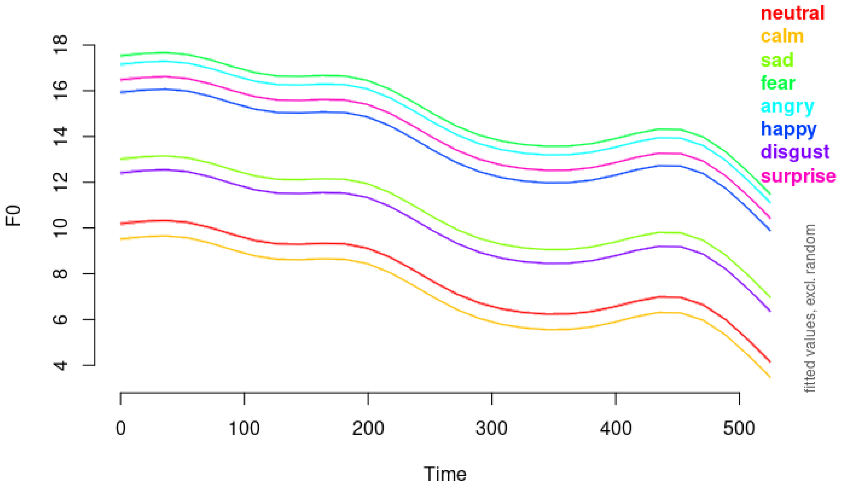
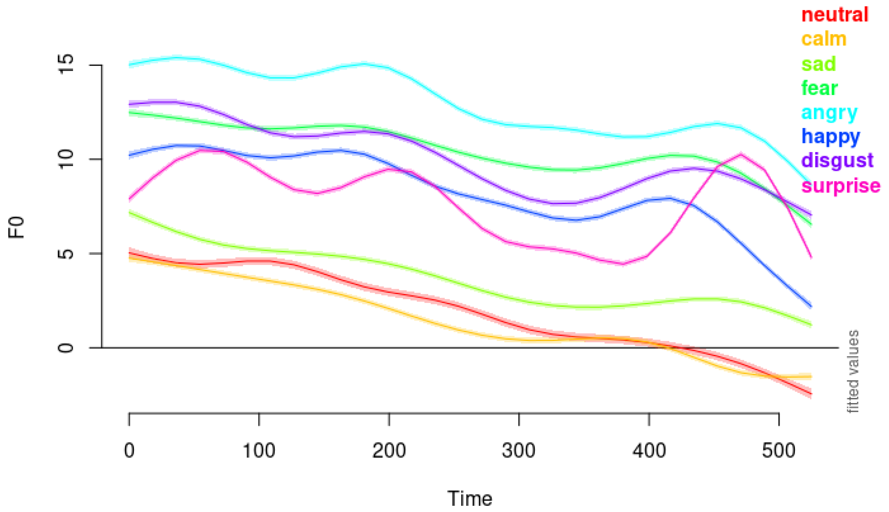
In our analysis, as illustrated in Figure 5 and Figure 6, we observed that anger, disgust, and fear all exhibit downward pitch contours at elevated pitch levels. Emotions such as sadness, calm, and neutral are characterized by downward pitch contours at subdued pitch levels. Notably, sadness occurs at a slightly higher pitch level than calm and neutral, which might reflect a difference in emotional arousal. The similarity between the pitch contours of calm and neutral suggests that these two emotions may be challenging to distinguish for listeners, potentially leading to misclassification. This difficulty underscores the importance of nuanced acoustic analysis in emotion recognition systems.

Among these emotions, anger starts at a higher pitch level than both disgust and fear, aligning partially with [8]’s findings regarding anger’s high pitch. While disgust also shows a downward contour similar to anger, it displays more fluctuation in the pitch contour compared to fear.

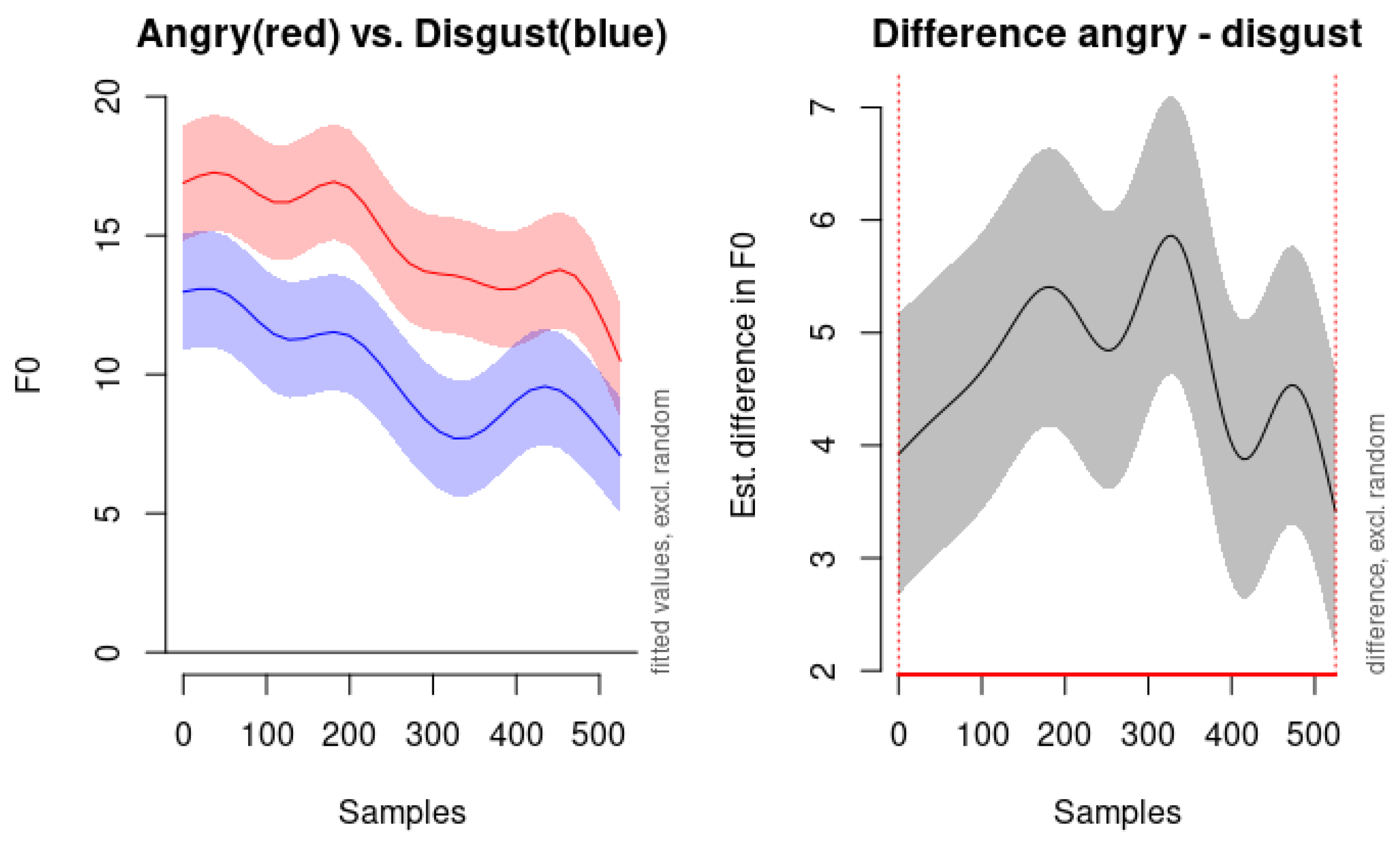
To further examine the nuances between anger and disgust, we present the modeled F0 contours for these emotions in Figure 7. As depicted in the left panel of Figure 7, both emotions demonstrate very similar shapes in their dynamic F0 movements, indicating a shared downward trajectory in pitch over time. However, the anger emotion (red line) consistently exhibits higher pitch levels compared to disgust (blue line) throughout the utterance.

The right panel of Figure 7 illustrates the estimated difference in the F0 between the angry and disgust conditions, along with the confidence interval of the difference. This visual comparison highlights that while the dynamic patterns of pitch movement are similar for both emotions, the overall pitch level serves as a distinguishing feature. The elevated pitch levels associated with anger support the notion of increased arousal and intensity in this emotion, which is reflected acoustically.

Interestingly, disgust in our data does not conform to the low mean pitch reported previously. In [8], disgust is expressed with a low mean pitch, a low intensity level, and a slower speech rate than the neutral state does. However, this is not the case in our data. Instead, it displays elevated pitch levels with more fluctuation in the pitch contour compared to fear. This discrepancy suggests that disgust may be expressed differently in the RAVDESS dataset, potentially due to cultural, linguistic, or methodological differences. The expression and perception of emotions can vary across cultures and languages. What is considered a typical acoustic manifestation of an emotion in one culture may differ in another. Or it can be the case that the actors in the RAVDESS dataset may have employed a different vocal strategy to convey disgust, perhaps emphasizing certain prosodic features to make the emotion more discernible. Methodological differences may have led to the differences in the finding; our use of dynamic modeling with GAMMs allows for capturing temporal variations in pitch contours that static measures like mean pitch may overlook.

The acoustic properties of calm and sadness emotions are characterized by downward pitch contours at subdued pitch levels, reflecting their low arousal states. This downward trajectory in pitch aligns with previous research indicating that lower pitch and reduced variability are common in less active or more negative emotional states. However, there are notable differences between the two emotions. Sadness consistently exhibits a slightly higher pitch level than calm throughout the utterance. This elevated pitch in sadness may convey a sense of emotional weight or poignancy, distinguishing it from the more neutral or relaxed state of calm. While both emotions are low in arousal, sadness typically carries a negative valence, whereas calm is generally neutral or slightly positive. This difference in emotional valence might be subtly reflected in the acoustic properties, such as the slight elevation in pitch for sadness.

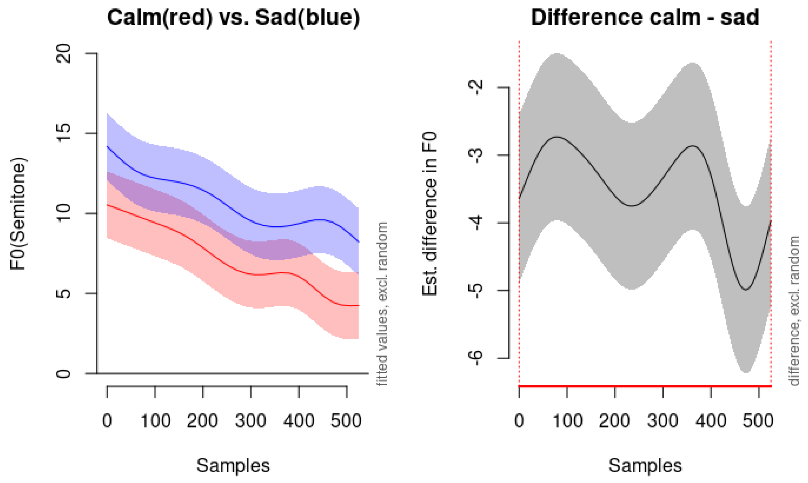
As illustrated in Figure 8, the left panel displays the fitted pitch contours for calm (red line) and sadness (blue line) over 500 samples. Both contours demonstrate a similar downward trend, but the pitch level for sadness remains consistently higher than that of calm. The shaded areas represent the confidence intervals excluding random effects, showing the reliability of these observations. The right panel of Figure 8 presents the estimated difference in the F0 between the calm and sad conditions, with the shaded area indicating the confidence interval of the difference. The fact that the confidence interval does not cross zero throughout the entire time window (0 to 525 samples) suggests that the difference in pitch level between calm and sadness is statistically significant across the utterance. These findings highlight the similarities between calm and sadness in terms of pitch contour shape: both exhibit a downward slope indicative of low arousal. However, the differences in the overall pitch level provide an acoustic cue for distinguishing between the two emotions. The higher pitch in sadness may reflect a slight increase in emotional intensity or a different emotional valence compared to calm.

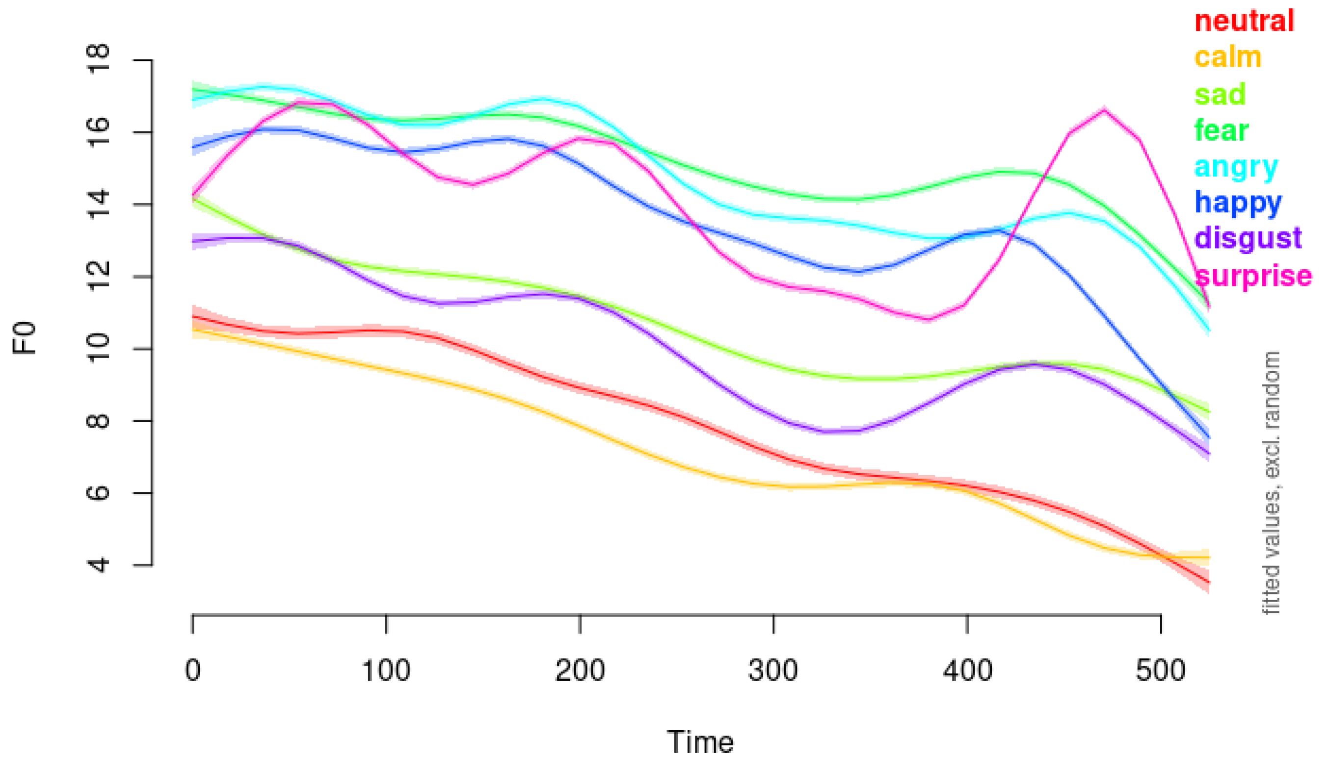
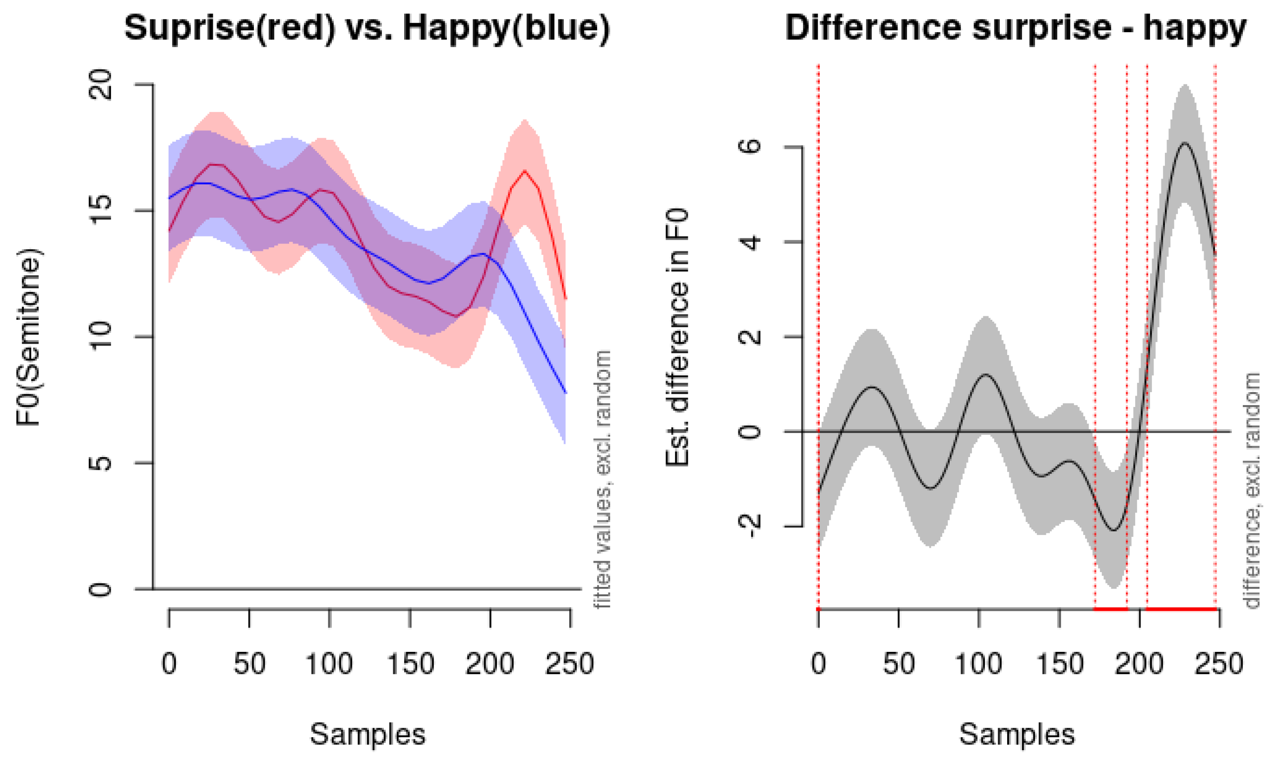
In our study, the pitch contours of happiness and surprise display distinct characteristics that aid in differentiating these emotions acoustically. The pitch contour of happiness begins at a mid-level pitch and exhibits a steeper downward slope compared to other emotions. This pattern aligns with previous research suggesting that happiness involves increased pitch variability and dynamic intonation patterns, reflecting a cheerful and expressive vocal demeanor. In contrast, the pitch contour of surprise is notably distinctive. As illustrated in Figure 9, surprise shows significant fluctuation throughout the utterance and features an elevated pitch towards the end, surpassing even other high-activation emotions like anger and fear. This elevation in pitch at the conclusion of the utterance may mirror the suddenness and heightened intensity typically associated with surprise. The dynamic rise in pitch could be indicative of an exclamatory expression, which is characteristic of how surprise is often vocally manifested.

The left panel of Figure 9 demonstrates the fitted pitch contours for both emotions. While both happiness and surprise start at similar pitch levels, their trajectories diverge significantly over time. Happiness maintains a relatively steady pitch before descending sharply, whereas surprise exhibits considerable fluctuation and culminates in a pronounced pitch increase at the end. The right panel of Figure 9 highlights the estimated difference in the F0 between the two emotions. The areas where the confidence interval does not cross zero indicate time windows where the difference in pitch is statistically significant. These differences suggest that listeners may rely on the distinctive pitch patterns, particularly the end-of-utterance elevation in surprise, to differentiate it from happiness.

Our results emphasize the importance of considering both the shape and level of pitch contours in emotion recognition. The similarities in contour shape indicate that relying solely on the dynamic movement of pitch may not suffice for accurate classification between certain emotions. However, incorporating pitch level differences enhances the discriminative power of the model, enabling better differentiation between closely related emotional expressions like anger and disgust. The unique pitch elevation in surprise, contrasted with the steeper downward slope in happiness, provides acoustic cues that are critical for distinguishing between these two positive high-arousal emotions. This differentiation is crucial, as happiness and surprise can be easily confused due to their shared characteristics of high activation and positive valence.

Our use of Generalized Additive Mixed Models (GAMMs) allows us to capture nuanced acoustic differences among various emotional states. By modeling the dynamic F0 contours, we enhance the interpretability of the emotion classification system, providing insights into how specific acoustic features correspond to different emotions. This approach is particularly valuable for low-arousal emotions like calm and sadness, where acoustic differences are more subtle and require sophisticated modeling techniques to detect.

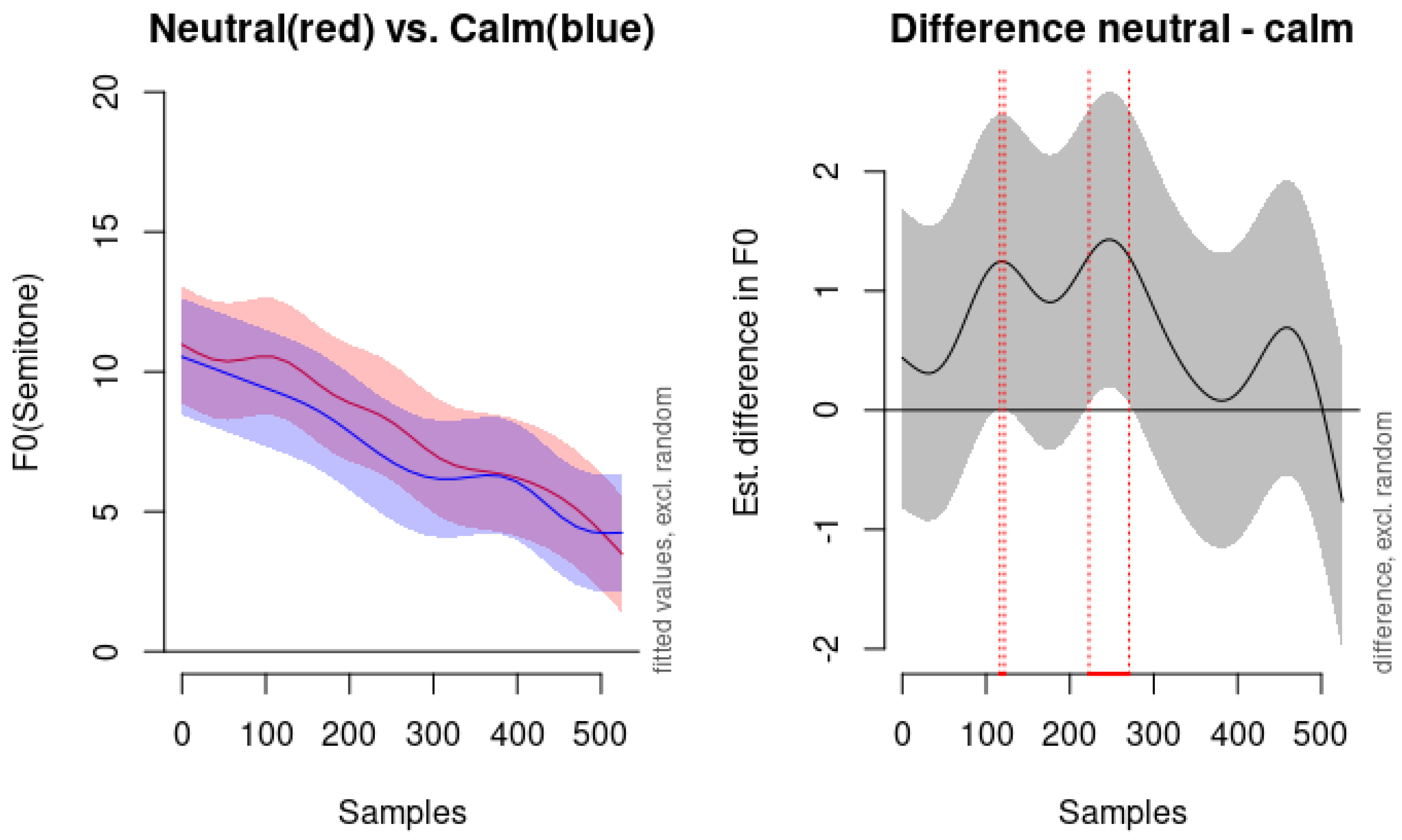
One of the challenges we encountered is the differentiation between neutral and calm emotions. According to our modeling, the neutral emotion is not statistically significantly different from calm emotion. As shown in Figure 10, which compares the predicted F0 contours for neutral and calm, the pitch contours are remarkably similar. The right panel of Figure 10 indicates with vertical red dots that the time window of significant difference is found merely between 116.67 and 121.97 milliseconds as well as 222.73 and 270.45 milliseconds: a very brief duration overall. The following observation from [29] provides context for our findings: The inclusion of both neutral and calm emotions in the RAVDESS dataset acknowledges the challenges that performers and listeners face in distinguishing these states. The minimal acoustic differences captured by our GAMM analysis reflect this perceptual similarity, as noted in [2] (note that in the quotation, the author’s citation style is replaced with numeric style citation):

“[T]he RAVDESS includes two baseline emotions, neutral and calm. Many studies incorporate a neutral or ‘no emotion’ control condition. However, neutral expressions have produced mixed perceptual results [1], at times conveying a negative emotional valence. Researchers have suggested that this may be due to uncertainty on the part of the performer as to how neutral should be conveyed [3]. To compensate for this, a calm baseline condition has been included, which is perceptually like neutral but may be perceived as having a mild positive valence. To our knowledge, the calm expression is not contained in any other set of dynamic conversational expressions” [29].

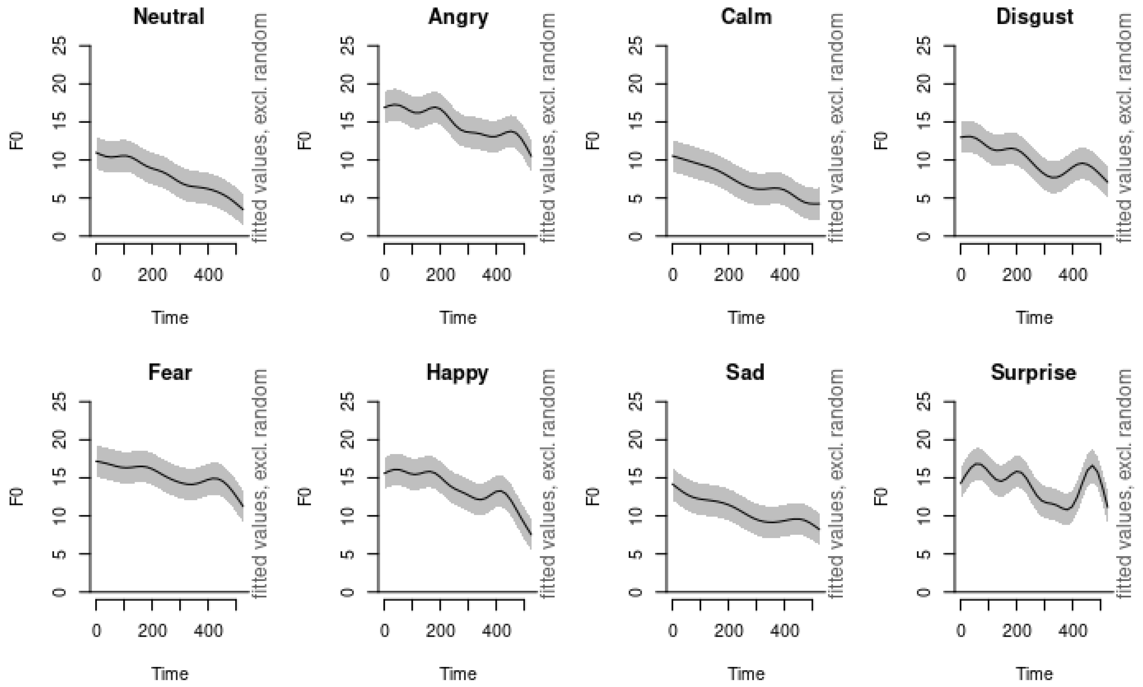
Figure 10 illustrates the modeled F0 contours and differences between neutral and calm emotions. The left panel displays the fitted pitch values in semitones over 500 samples, with shaded areas representing the confidence intervals, excluding random effects. The contours for neutral (red line) and calm (blue line) are nearly overlapping, indicating highly similar pitch patterns. The right panel shows the estimated difference in the F0 between the neutral and calm conditions, with the shaded area indicating the confidence interval of the difference. The vertical red dots mark the brief time windows where the difference is statistically significant.

Additionally, Figure 10 also includes comparisons of the modeled F0 contours for angry and happy emotions (top panel), demonstrating how our method effectively captures and illustrates distinctions between emotions with higher arousal levels. The clear differences in pitch contours and levels between angry and happy support the effectiveness of GAMMs in modeling and interpreting emotional speech across the arousal spectrum.

In conclusion, our use of GAMMs facilitates a deeper understanding of the acoustic properties of emotional speech. By capturing both prominent and subtle differences among emotions, especially in cases where traditional statistical methods might overlook minor yet significant variations, our approach enhances both the interpretability and the accuracy of emotion classification systems.

5. Conclusions

In this study, we employed a Generalized Additive Mixed Model (GAMM) to analyze the role of dynamic F0 contours in the classification of eight basic emotions using the RAVDESS corpus. The F0 values, extracted over the sonorant portions of speech at ten equidistant points, were concatenated across two predetermined sentences. By focusing on these controlled utterances, we aimed to isolate the effect of pitch dynamics on emotion recognition.

Our findings confirm previous observations about the informative role of pitch in expressing emotions. The dynamic modeling of F0 contours provided insights into the specific acoustic patterns associated with different emotional states. For instance, we observed that emotions such as anger, disgust, and fear exhibit downward pitch contours at elevated pitch levels, while happiness displays a steeper downward slope starting from a mid-level pitch. These nuanced differences highlight the significance of dynamic pitch features in distinguishing between emotions.

One of the key advantages of our approach is its interpretability. While deep learning-based automatic speech recognition systems have achieved higher accuracy in classifying emotion types—surpassing both human raters and our pitch contour-based modeling—they often function as “black boxes,” offering limited insight into the features driving their performance. In contrast, our method allows for a more transparent understanding of why certain emotions are harder to distinguish than others. By directly modeling dynamic F0 contours, we can explain, for example, why emotions like calm and neutral are challenging to differentiate due to their similar pitch patterns.

However, our study also has limitations that warrant discussion. The analysis was conducted using predetermined sentences, which constrains the generalizability of our findings to a broader range of speech contexts. The use of controlled utterances, while beneficial for isolating specific acoustic features, may not capture the variability inherent in natural, spontaneous speech. This limitation suggests that caution should be exercised when extrapolating our results to more diverse linguistic environments.

Despite this constraint, focusing on fixed sentences provided a controlled setting to delve deeply into the role of dynamic F0 in emotion classification. It allowed us to attribute differences in emotion recognition specifically to pitch contours, minimizing the influence of lexical or syntactic variations. This approach contributes valuable insights into how dynamic pitch features function as acoustic correlates of emotional expression.

It is also important to acknowledge that pitch contour alone does not bear the entire burden of conveying expressive meaning in speech. Emotions are complex and multifaceted, often communicated through a combination of prosodic features such as intensity, duration, speech rate, and spectral qualities. While our study was solely restricted to the pitch contour variable—due to its significant role in arousing sensations in listeners and its previously underexplored modeling—it is clear that incorporating additional acoustic features could enhance emotion recognition systems.

Future research should consider expanding the scope of analysis to include other prosodic and spectral features. Integrating variables such as intensity, speech rate, and formant frequencies could provide a more comprehensive understanding of emotional speech. Additionally, applying dynamic modeling techniques like GAMMs to spontaneous speech samples or a wider variety of sentences could improve the generalizability of the findings and contribute to the development of more robust emotion recognition models. Additionally, including dynamic and multimodal properties could be an interesting area for future research. For example, ref. [41] achieved an 80.08% accuracy in classifying eight emotions on the RAVDESS dataset using a multimodal emotion recognition system that combines speech and a facial recognition model.

In conclusion, our study demonstrates that dynamic F0 contours play a crucial role in emotion classification and that modeling these contours using GAMMs offers both interpretability and valuable insights into the acoustic properties of emotional speech. While the use of predetermined sentences presents limitations in terms of generalizability, it also serves as a strength by providing a controlled environment to explore the impact of pitch dynamics. Our approach underscores the importance of transparent and interpretable models in speech emotion recognition, paving the way for future studies to build upon these findings and develop more sophisticated, multimodal emotion recognition systems.

References

1. Scherer, K.R.; Banse, R.; Wallbott, H.G.; Goldbeck, T. Vocal cues in emotion encoding and decoding. Motiv. Emot. 1991, 15, 123–148. [Google Scholar] [CrossRef]
2. Ekman, P. Are there basic emotions? Psychol. Rev. 1992, 99, 550–553. [Google Scholar] [CrossRef] [PubMed]
3. Juslin, P.N.; Laukka, P. Communication of emotions in vocal expression and music performance: Different channels, same code? Psychol. Bull. 2003, 129, 770–814. [Google Scholar] [CrossRef] [PubMed]
4. Yoon, S.; Son, G.; Kwon, S. Fear emotion classification in speech by acoustic and behavioral cues. Multimed. Tools Appl. 2019, 78, 2345–2366. [Google Scholar] [CrossRef]
5. Plutchik, R. A general psychoevolutionary theory of emotion. In Theories of Emotion; Plutchik, R., Kellerman, H., Eds.; Academic Press: New York, NY, USA, 1980; pp. 3–33. [Google Scholar]
6. Russell, J.; Bachorowski, J.; Fernández-Dols, J. Facial and vocal expressions of emotion. Annu. Rev. Psychol. 2003, 54, 329–349. [Google Scholar] [CrossRef]
7. Tomkins, S. Affect Imagery Consciousnesss: Volume I: The Positive Affects; Springer Publishing Company: New York, NY, USA, 1962. [Google Scholar]
8. Ververidis, D.; Kotropoulos, C. Emotional Speech Recognition: Resources, Features, and Methods. Speech Commun. 2006, 48, 1162–1181. [Google Scholar] [CrossRef]
9. Davis, S.; Mermelstein, P. Evaluation of acoustic parameters for monosyllabic word identification. J. Acoust. Soc. Am. 1978, 64 (Suppl. 1), S180–S181. [Google Scholar] [CrossRef]
10. Abdulmohsin, H. A new proposed statistical feature extraction method in speech emotion recognition. Comput. Electr. Eng. 2021, 93, 107172. [Google Scholar] [CrossRef]
11. Alsalhi, A.; Almehmadi, A. Using Vocal-Based Emotions as a Human Error Prevention System with Convolutional Neural Networks. Appl. Sci. 2024, 14, 5128. [Google Scholar] [CrossRef]
12. Rodero, E. Intonation and Emotion: Influence of Pitch Levels and Contour Type on Creating Emotions. J. Voice 2011, 25, e25–e34. [Google Scholar] [CrossRef]
13. Whissel, C. The dictionary of affect in language. In Emotion: Theory, Research and Experience; Plutchik, R., Kellerman, H., Eds.; Academic Press: New York, NY, USA, 1989; Volume 4, pp. 113–131. [Google Scholar]
14. Juslin, P.N.; Laukka, P. Impact of intended emotion intensity on cue utilization and decoding accuracy in vocal expression of emotion. Emotion 2001, 1, 381–412. [Google Scholar] [CrossRef] [PubMed]
15. Arias, J.P.; Busso, C.; Yoma, N.B. Shape-based modeling of the fundamental frequency contour for emotion detection in speech. Comput. Speech Lang. 2014, 28, 278–294. [Google Scholar] [CrossRef]
16. Bänziger, T.; Scherer, K.R. The role of intonation in emotional expressions. Speech Commun. 2005, 46, 252–267. [Google Scholar] [CrossRef]
17. Hirose, K.; Sato, K.; Asano, Y.; Minematsu, N. Synthesis of F0 contours using generation process model parameters predicted from unlabeled corpora: Application to emotional speech synthesis. Speech Commun. 2005, 46, 385–404. [Google Scholar] [CrossRef]
18. Paeschke, A.; Kienast, M.; Sendlmeier, W.F. F0-contours in emotional speech. In Proceedings of the 14th International Congress of Phonetic Sciences, Melbourne, Australia, 5–9 August 2019; pp. 929–932. [Google Scholar]
19. Sethu, V.; Ambikairajah, E.; Epps, J. On the use of speech parameter contours for emotion recognition. EURASIP J. Audio Speech Music Proc. 2013, 2013, 19. [Google Scholar] [CrossRef]
20. Morrison, G.S. L1-Spanish Speakers’ Acquisition of the English /i/—/I/ Contrast: Duration-based perception is not the initial developmental stage. Lang. Speech 2008, 51, 285–315. [Google Scholar] [CrossRef]
21. Wood, S.N. Generalized Additive Models: An Introduction with R; Chapman and Hall/CRC: New York, NY, USA, 2017. [Google Scholar] [CrossRef]
22. van Rij, J. Overview GAMM Analysis of Time Series Data. Available online: https://jacolienvanrij.com/Tutorials/GAMM.html (accessed on 23 October 2023).
23. Chuang, Y.; Fon, J.; Papakyritsis, I.; Baayen, H. Analyzing phonetic data with generalized additive mixed models. In Manual of Clinical Phonetics; Ball, M., Ed.; Routledge: London, UK, 2021; pp. 108–138. [Google Scholar] [CrossRef]
24. Shegokar, P.; Sircar, P. Continuous wavelet transform based speech emotion recognition. In Proceedings of the 2016 10 International Conference on Signal Processing and Communication Systems (ICSCS), Surfers Paradise, Australia, 19–21 December 2016; pp. 1–8. [Google Scholar] [CrossRef]
25. Zhang, B.; Provost, E.M.; Essi, G. Cross-corpus acoustic emotion recognition from singing and speaking a multi-task learning approach. In Proceedings of the 2016 IEEE International Conference on Acoustics, Speech, and Signal Processing (ICASSP), Shanghai, China, 20–25 March 2016; pp. 5805–5809. [Google Scholar] [CrossRef]
26. Zeng, Y.; Mao, H.; Peng, D.; Yi, Z. Spectrogram based multi-task audio classification. Multimed. Tools Appl. 2019, 78, 3705–3722. [Google Scholar] [CrossRef]
27. Popva, A.S.; Rassadin, A.G.; Ponomarenko, A.A. Emotion recognition in sound. In Proceedings of the International Conference on Neuroinformatics, Moscow, Russia, 2–6 October 2017; pp. 117–124. [Google Scholar]
28. Issa, D.M.; Yazici, A. Speech emotion recognition with deep convolutional neural networks. Biomed. Signal Process. Control 2020, 59, 101894. [Google Scholar] [CrossRef]
29. Livingstone, S.R.; Russo, F.A. The Ryerson Audio-Visual Database of Emotional Speech and Song (RAVDESS): A dynamic, multimodal set of facial and vocal expressions in North American English. PLoS ONE 2018, 13, e0196391. [Google Scholar] [CrossRef]
30. Jadoul, Y.; Thompson, B.; de Boer, B. Introducing Parselmouth: A Python interface to Praat. J. Phon. 2018, 71, 1–15. [Google Scholar] [CrossRef]
31. McFee, B.; Raffel, C.; Liang, D.; Ellis, D.; McVicar, M.; Battenbert, E.; Nieto, O. librosa: Audio and music signal analysis in python. In Proceedings of the 14th Python in Science Conference, Austin, TX, USA, 6–12 July 2015. [Google Scholar]
32. Buschmeier, H.; Wlodarczak, M. TextGridTools: A TextGrid processing and analysis toolkit for Python. In Proceedings of the Tagungsband der 24, Konferenz zur Elektronischen Sprachsignalverarbeitung (ESSV 2013), Bielefeld, German, 26–28 March 2013. [Google Scholar]
33. Boersma, P.; Weenink, D. Praat: Doing Phonetics by Computer [Computer Program Version 6.1.38]. Available online: http://www.praat.org/ (accessed on 2 January 2021).
34. McFee, B. resampy: Efficient sample rate conversion in Python. J. Open Source Softw. 2016, 1, 125. [Google Scholar] [CrossRef]
35. van Rij, J.; Wieling, M.; Baayen, R.H.; van Rijn, H. itsadug: Interpreting Time Series and Autocorrelated Data using GAMMs. 2022. R package version 2.4.1. Available online: https://rdrr.io/cran/itsadug/ (accessed on 22 November 2024).
36. Stuart-Smith, J.; Lennon, R.; Macdonald, R.; Robertson, D.; Sóskuthy, M.; José, B.; Evers, L. A dynamic acoustic view of 528 real-time change in word-final liquids in spontaneous Glaswegian. In Proceedings of the 18th International Congress of Phonetic Sciences, Glasgow, UK, 10–14 August 2015. [Google Scholar]
37. Wieling, M. Analyzing dynamic phonetic data using generalized additive mixed modeling: A tutorial focusing on articulatory differences between L1 and L2 speakers of English. J. Phon. 2018, 70, 86–116. [Google Scholar] [CrossRef]
38. Baayen, H.; Vasishth, S.; Kliegl, R.; Bates, D. The cave of shadows: Addressing the human factor with generalized additive mixed models. J. Mem. Lang. 2017, 94, 206–234. [Google Scholar] [CrossRef]
39. Sóskuthy, M. Evaluating generalised additive mixed modelling strategies for dynamic speech analysis. J. Phon. 2021, 84, 101017. [Google Scholar] [CrossRef]
40. Winter, B.; Wieling, M. How to analyze linguistic change using mixed models, Growth Curve Analysis and Generalized Additive Modeling. J. Lang. Evol. 2016, 1, 7–18. [Google Scholar] [CrossRef]
41. Luna-Jiménez, C.; Griol, D.; Callejas, Z.; Kleinlein, R.; Montero, J.M.; Fernández-Martínez, F. Multimodal emotion recognition on RAVDESS dataset using transfer learning. Sensors 2021, 21, 7665. [Google Scholar] [CrossRef]
Figure 1. Left panel: Sample of F0 values in semitones extracted from the audio file “03-01-08-01-01-01-03.wav.” Right panel: Resampled pitch contours using the resampy function. The pitch values in semitone, which are randomly generated for an illustrative purpose, are represented by the solid line, and the resampled pitch values are represented by the dotted line. The X-axis on both panels represents frames.
Applsci 14 10972 g001
Figure 2. Boxplot of mean F0 (semitones) for each emotion category. The dot inside each box denotes the mean F0 for that emotion.
Applsci 14 10972 g002
Figure 3. The modeled F0 trends over time only.
Applsci 14 10972 g003
Figure 4. The modeled F0 contours over time for each emotion, estimated using Model 2.
Applsci 14 10972 g004
Figure 5. The modeled F0 contours over time for each emotion, estimated using Model 4.
Applsci 14 10972 g005
Figure 6. F0 contours of each emotional type modeled with Model 4.
Applsci 14 10972 g006
Figure 7. Comparison of pitch contours between angry (red) and disgust (blue) speech samples. The left panel displays the fitted pitch values in semitones over 500 samples, with shaded areas representing the confidence intervals, excluding random effects. The right panel shows the estimated difference in the F0 (fundamental frequency) between the angry and disgust conditions, with the shaded area indicating the confidence interval of the difference.
Applsci 14 10972 g007
Figure 8. Comparison of pitch contours between calm (red) and sad (blue) speech samples. The left panel displays the fitted pitch values in semitones over 500 samples, with shaded areas representing the confidence intervals, excluding random effects. The right panel shows the estimated difference in the F0 (fundamental frequency) between the calm and sad conditions, with the shaded area indicating the confidence interval of the difference.
Applsci 14 10972 g008
Figure 9. Comparison of pitch contours between surprise (red) and happy (blue) speech samples. The left panel displays the fitted pitch values in semitones over 500 samples, with shaded areas representing the confidence intervals, excluding random effects. The right panel shows the estimated difference in the F0 (fundamental frequency) between the surprise and happy conditions, with the shaded area indicating the confidence interval of the difference.
Applsci 14 10972 g009
Figure 10. Comparison of pitch contours between neutral (red) and calm (blue) speech samples. The left panel displays the fitted pitch values in semitones over 500 normalized time points, with shaded areas representing the 95% confidence intervals (excluding random effects). The right panel shows the estimated difference in the F0 (fundamental frequency) between the neutral and calm conditions, with the shaded area indicating the 95% confidence interval of the difference. Vertical red lines denote time windows where the difference is statistically significant.
Applsci 14 10972 g010