Underwater Acoustic Signal LOFAR Spectrogram Denoising Based on Enhanced Simulation

Abstract

In complex marine environments, extracting target features from acoustic signal is very difficult, making the targets hard to be recognized. Therefore, it is necessary to perform denoising method on the acoustic signal to highlight the target features. However, training deep learning denoising models requires a large mount of acoustic data with labels and obtaining labels with real measured data is also extremely difficult. In this paper, an enhanced simulation algorithm, which considers integrating features of target line spectrum and ocean environmental noise, is proposed to construct a large-scale training sample set. Additionally, a deep convolutional denoising model is presented, which is first train on simulated data and directly applied to real measured data for denoising, enabling line spectrum to be significantly displayed in the time-frequency spectrogram. The results on simulation experiments and sea trials demonstrate that the proposed method can significantly reduce ocean noise while preserving the characteristics of target line spectrum. Furthermore, the experiments demonstrate that the proposed convolutional denoising model has transferability and generalization, making it suitable for denoising underwater acoustic signal in different marine areas.

1. Introduction

Underwater acoustic target detection and recognition based on passive sonar plays an important role in underwater confrontation and maritime surveillance. The LOFAR (Low Frequency Analysis and Recording) spectrogram, as one of the important analytical tools for ocean target detection, uses Short-Time Fourier Transform (STFT) to extract and transform the target radiated noise, resulting in a time-frequency spectrogram. line spectrum in the LOFAR spectrogram is used to determine the type of target [1,2,3,4,5,6]. However, with the advancement of marine engineering noise reduction technology, high-frequency noise from marine equipment has been effectively suppressed, significantly enhancing the quietness of the equipment itself. In complex marine environments, the target line spectrum tends to become unclear. Therefore, how to denoise signal based on LOFAR spectrograms is of great significance.

Underwater acoustic denoising methods are mainly divided into two categories: traditional decomposition methods and deep learning methods. Traditional decomposition methods, including discrete wavelet transform (DWT) [7], empirical mode decomposition (EMD) [8], variational mode decomposition (VMD) [9], and empirical wavelet transform (EWT) [10], break complex signals into multiple components, which are then processed by denoising techniques and reassembled to reconstruct the clean signal. As deep learning advances, reseachers are exploring methods for enhancing target line spectrum or reducing marine noise by letting the model learn a mapping from noisy data to clean data. By combining the principles of Adaptive Line Enhancer (ALE), Ju et al. [11] design unsupervised learning line spectrum enhancer to enhance line spectrum components under low signal-to-noise ratio conditions. Yang et al. [12] use a bidirectional Long Short-Term Memory (LSTM) model for LOFAR spectrogram denoising. Li et al. [13] study the denoising method of pulse signal in non-Gaussian environments by establishing a convolutional neural network that learns the residual mapping between the short-time Fourier transform features of pure signal and received signal, achieving noise suppression. Yin et al. [14] combine autoencoders with convolution, inputting time-domain signal to retain amplitude and phase information, thereby reducing noise components in signal. Cao et al. [15] optimize the shape of convolution kernels in convolutional autoencoders to better adapt to line spectrum features, applying this to the classification and identification of LOFAR spectrogram. Luo [16] compares the denoising effects of Deep Neural Network (DNN) and DnCNN (Denoising Convolutional Neural Network) under different signal-to-noise ratio conditions. Jiang et al. [17] apply Generative Adversarial Networks (GANs) to underwater acoustic signal separation, introducing class condition constraints at the model input and discriminator loss at the output to enhance the quality of target separation. Gu et al. [18] proposed a time-frequency attention mechanism module utilizing both time-domain and frequency-domain information to enhance the model’s time-domain attention, addressing the detection of underwater low-noise quiet-type targets. The aforementioned methods focus on improving denoising techniques but overlook the differences between simulated and measured data. Using deep learning to remove noise requires obtaining a large amount of labeled target spectral signal data, which poses a challenge for deep learning modeling.

However, traditional decomposition methods are highly sensitive to parameter settings, which often leads to suboptimal denoising performance, especially in complex and dynamic environments. These methods can struggle to adapt to the varying characteristics of real-world signals, resulting in poor noise removal. Although deep learning-based approaches have shown superior performance in denoising acoustic signals, they come with significant drawbacks. One key issue is that these methods directly combine clean and noise signals to generate noisy data, neglecting the inherent complexity of real-world signals in practical environments. Additionally, deep learning techniques require large amounts of labeled training data, and acquiring high-quality, accurately, real-world labeled datasets is both time-consuming and costly, which limits their widespread application. To address the aforementioned issues, this paper proposes a LOFAR spectrogram denoising method for underwater acoustic signal based on simulation enhancement. By utilizing ocean noise collected during sea trials, and combining it with line spectrum simulation data, we construct a large-scale labeled training dataset required for model training. This dataset is then used to train an effective deep convolutional denoising model. The trained model is directly applied to the sea trial data for denoising, allowing line spectrum to be prominently extracted on the time-frequency spectrogram, facilitating target feature analysis and recognition.

The rest of paper is organized as follows: An enhanced simulation algorithm and convolutional denoising model that can significantly denoise environment noise in LOFAR spectrogram is proposed in Section 2. The experiment settings and datasets that used in this paper are elaborated in Section 3. In Section 4, quantitative results of experiments are presented. Finally, conclusions are summarized in Section 5.

2. Materials and Methods

The main framework of the proposed method is shown in Figure 1. First, based on the characteristics of line spectrum and ocean noise, the enhanced simulation algorithm fuses target acoustic data with ocean environmental noise data in both the time and frequency domains, constructing training and testing datasets. Next, the cross-entropy loss function is used as the optimization objective for the convolutional denoising model and train the model using gradient descent. Finally, the converged model is applied to obtain the line spectrum data of target and ocean noise.

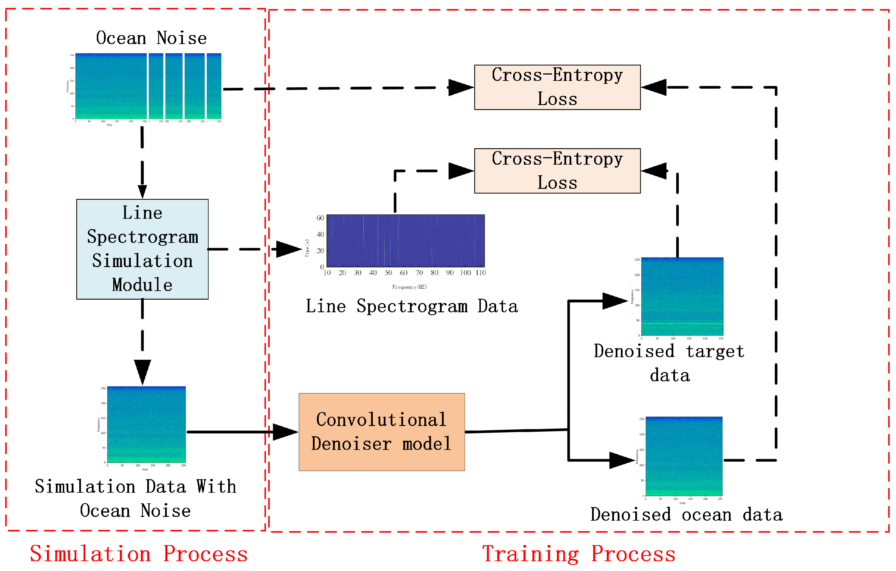
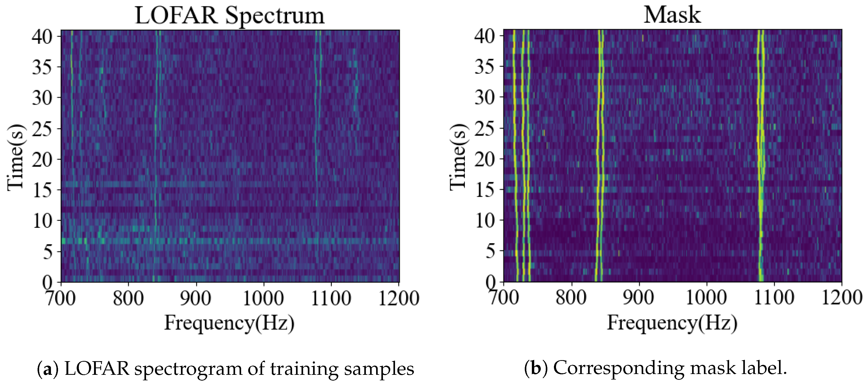
2.1. Training Data Simulation Method

The performance of deep neural network model is related to the quantity and quality of training samples. The completeness of the sample space directly affects the model’s generalization ability in practical applications, and high-quality simulated data should closely resemble actual measured data. However, due to the inherent complexity of the marine environment and the high costs of data labeling, it is difficult to obtain high signal-to-noise ratio (SNR) and low-noise sample pairs which are treated as model inputs and outputs to train robust deep neural networks for LOFAR spectrogram denoising. Therefore, during the data simulation phase, large-scale labeled training samples are created by combining target-free ocean environment noise with simulated line spectrum to train the denoising model.

If the signal is periodic or contains periodic components, it will manifest as a line spectrum in the time-frequency spectrogram. Therefore, a line spectrum can be represented by a single frequency signal $u\left(t\right)$:

$$u\left(t\right)=A\times sin(2\pi ft+\varphi )$$

(1)

where A represents the signal amplitude, f denotes the signal frequency, $\varphi$ represents the initial phase of the signal, and $t\in [0,T]$ represents time. In practical scenarios, the target does not always remain stationary. When the target is in relative motion with respect to the sonar, phase and frequency will change due to the difference in propagation distance, which is known as the Doppler frequency shift phenomenon, it can be defined as:

$$f^{\prime }={\displaystyle \frac{(v\pm v_0)}{(v\mp v_s)}}f$$

(2)

where $f^{\prime }$ is the frequency received by the sonar, f is the frequency of the noise radiated by the target in the water, v is the speed of sound waves in water; $v_0$ is the speed of the sonar relative to the water, and $v_s$ is the speed of the target relative to the sonar. Based on the Equation (2), $\Delta f$ can be used to express the changes in frequency, thus Equation (2) can be simplified as:

$$f^{\prime }=f+\Delta f$$

(3)

The LOFAR spectrogram is a time-frequency plot, while the frequency shift of the target line spectrum exhibits an irregular phenomenon in the time dimension. However, regardless of the trend of frequency shift variations, the frequency of the line spectrum does not undergo significant changes and is severely offset from the center frequency. Therefore, this phenomenon can be described using a random walk, and the frequency drift variable $\Delta f$ satisfies:

$$E(\Delta f)=\sum _{t=1}^{T}E(\Delta f_t)=0$$

(4)

where $\Delta f_t$ represents the frequency drift of a single spectrogram line at time t and $E(·)$ stands for expectation. Similarly, affected by environmental noise and other factors, it is assumed that the amplitude of the single spectrogram line also follows a random walk process, defined as:

$$E(\Delta A)=\sum _{t=1}^{T}E(\Delta A_t)=0$$

(5)

where $\Delta A_t$ represents the amplitude drift of a single spectrogram line at time t. The initial phase $\varphi$ of the signal can be represented by a random number. Therefore, considering the frequency drift, the time-domain acoustic signal simulation algorithm for underwater targets is shown in Algorithm 1.

Algorithm 1 Time-Domain Underwater Acoustic Target Data Simulation Algorithm

Input: Signal duratio T, Sampling rate $f_s$, Lower frequency limit $f_l$, Upper frequency limit $f_h$, Lower amplitude limit $A_l$, Upper amplitude limit $A_h$, Number of spectrogram lines N, Amplitude of frequency drift $f_d$, Amplitude of amplitude drift $A_d$. Output: Time-Domain underwater acoustic target data: S. Initialize:$t=\left[0,{\displaystyle \frac{1}{f_s}},{\displaystyle \frac{2}{f_s}},\dots ,T\right]$//Initialize for a duration of T seconds.                $U=[0,0,\dots ,0]$ //Initialize the signal with duration T seconds Procedure: for i = 1 to N do     $f=\mathrm{random}(f_l,f_h)$            //Random center frequency value     $A=\mathrm{random}(A_l,A_h)$            //Random signal amplitude value     $\varphi =\mathrm{random}(0,\pi )$            //Random initial phase     for $j=1$ to $(f_s·T)$ do       //Signal duration of T seconds          if $jmod{f}_s=0$ then             $r_n=random(0,1)$             //Random value controlling direction             if $r_n\ge 0.5$ then                 $\delta =1$             //Random walk direction             else                 $\delta =-1$             //Random walk direction             end if             $f=f+\delta ·f_d$             //Frequency random walk             $A=A+\delta ·A_d$             //Amplitude random walk             $U\left[j\right]=U\left[j\right]+A·sin\left(2\pi ft\right[j]+\varphi )$  //Simulate one second data         end if     end for end for

Based on the simulation method, the time-domain acoustic signal of underwater target can be simulated. Due to the difference in average power between the simulated underwater target signal and the average power of the ocean noise, it is necessary to consider the impact of power when merging the simulated target signal with the ocean noise. This will ensure that the final simulated data can cover various signal-to-noise ratio conditions.

The signal-to-noise ratio of a known signal is defined as:

$$SNR=10{log}_{10}\left({\displaystyle \frac{P_{\mathrm{target}}}{P_{\mathrm{noise}}}}\right)=20{log}_{10}\left({\displaystyle \frac{A_{\mathrm{target}}}{A_{\mathrm{noise}}}}\right)$$

(6)

where $P_{\mathrm{target}}$ is the power of the target signal, $P_{\mathrm{noise}}$ is the power of the noise, $A_{\mathrm{target}}$ is the amplitude of the target signal, and $A_{\mathrm{noise}}$ is the amplitude of the noise. According to Equation (6), to obtain an accurate numerical value for the signal-to-noise ratio, the ratio of the amplitudes of the target signal to the noise should be adjusted, thus the adjustment coefficient $coef$ is defined as:

$$\mathrm{coef}=e^{{\displaystyle \frac{SN{R}_{\mathrm{target}}-20{log}_{10}\left(\frac{A_{\mathrm{target}}}{A_{\mathrm{noise}}}\right)}{20}}}$$

(7)

where $SN{R}_{\mathrm{target}}$ is the target signal-to-noise ratio from the simulation data. Thus, the final time-domain simulation signal S can be defined as:

$$S=coef\times U+Noise$$

(8)

where $Noise$ is the time-domain signal of ocean environmental noise. Based on above simulation methods and processes, the time-domain signal with an exact signal-to-noise ratio can be simulated, and the LOFAR spectrogram can be obtained through short-time Fourier transform as model input. In the training of the convolutional denoising model, not only input sample data is required, but also corresponding label samples. The aforementioned samples are obtained based on the simulation methods, so the label of the signal are also known. Additionally, since the denoising model operates on the LOFAR spectrogram, its label are presented in the form of spectrograms, which include a time-frequency representation with target-only line spectrum defined in Equation (9) and noise only spectrogram defined in Equation (10).

$${Mask}_{target}={\displaystyle \frac{\left|\right|STFT\left(U\right)\left|\right|}{\left|\right|STFT\left(U\right)\left|\right|+\left|\right|STFT\left(Noise\right)\left|\right|}}$$

(9)

$${Mask}_{noise}=1-{Mask}_{target}$$

(10)

where $Mas{k}_{target}$ represents the soft threshold mask label for the target, $Mas{k}_{noise}$ represents the soft threshold mask label for the noise, and $STFT(·)$ represents the short-time Fourier transform.

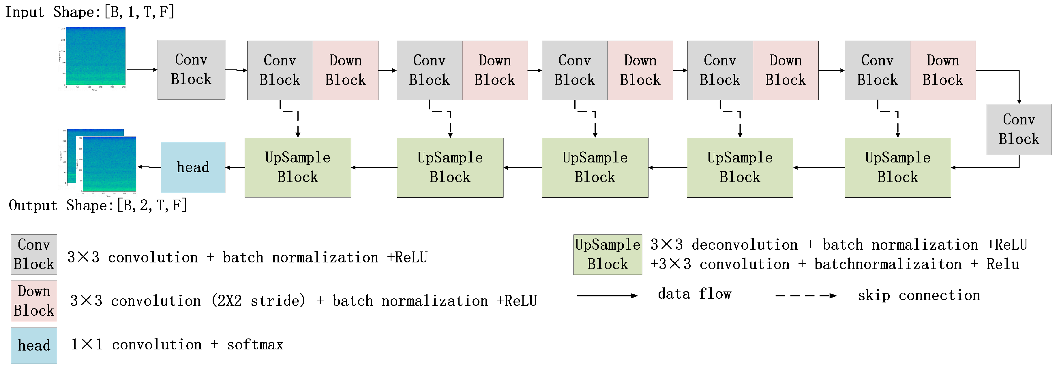
2.2. Convolutional Denoising Model

For LOFAR spectrogram $Y(T,F)$, it can be represented using the LOFAR spectrogram of the underwater target signal $X(T,F)$ and the additive ocean noise $N(T,F)$.

$$Y(T,F)=X(T,F)+N(T,F)$$

(11)

For the convolutional denoising model $M(·)$, the objective function $L(\theta ;Y,X)$ is to minimize the error between the LOFAR spectrogram of the underwater target signal and the LOFAR spectrogram predicted by the model.

$$L(\theta ;Y,X)=\underset{\theta }{min}{∥M\left(Y\right(T,F\left)\right)-X(T,F)∥}^2$$

(12)

Here, $\theta$ represents the parameters of the convolutional denoising model. For the image-to-image end-to-end problem, a deep convolutional network with a U-Net [19] like structure can be used. First, the encoder learns the feature representations from the spectrogram of raw acoustic signal. Then, the decoder reconstructs the feature representations into the LOFAR spectrogram of the underwater target sound signal. The structure diagram of the convolutional denoising model is shown in Figure 2.

In denoising model, the input dimension is $[B,1,T,F]$, where B is the batch size, T is the duration of the LOFAR spectrogram, and F is the frequency bandwidth. During the encoding phase, the input data undergoes a series of $3\times 3$ convolutions, ReLU (rectified linear unit) activation functions, and Batch Normalization. The downsampling module in the encoding phase employs $2\times 2$ stride convolutions instead of $1\times 1$ stride convolutions because $2\times 2$ stride convolutions have the capability to combine information from adjacent regions, reduce the size of the feature map, and extract more representative features. The first half of the model is the data encoding phase, where it is expected that the model learns a sparse representation of the data. In the second half of the model, known as the decoding phase, the decoder uses a combination of transposed convolutions, ReLU activation functions, and Batch Normalization, with the aim of separating the sparse representation into pure target signal and ocean noise. In the final layer of the model, a $1\times 1$ convolution and softmax function are used to generate a binary mask for the spectrogram. The dimension if final output is $[B,2,T,F]$, where 2 represents two spectrograms of the same size: the first spectrogram represents the foreground LOFAR spectrogram containing only the target line spectrum, while the second spectrogram represents the background LOFAR spectrogram containing only ocean environmental noise.

3. Experiments and Analysis

3.1. Experimental Settings

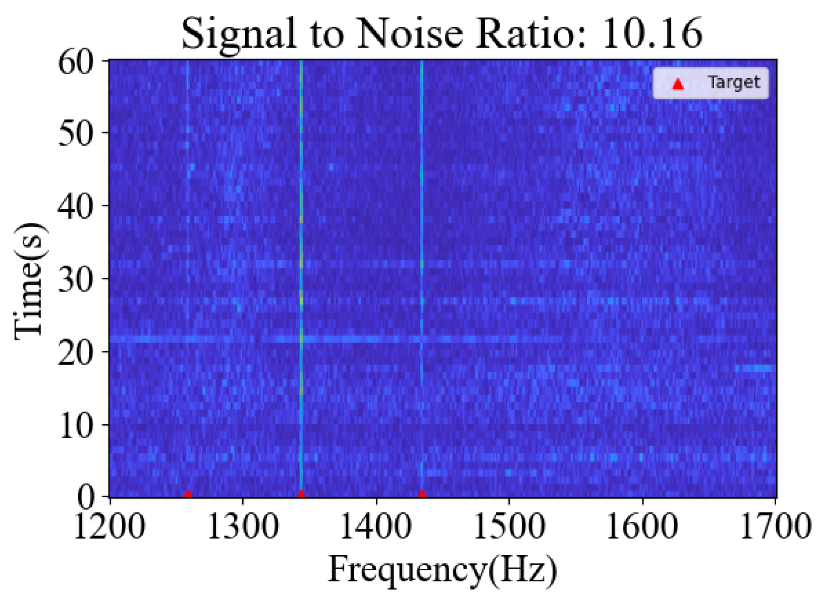
The experimental hardware conditions include an Nvidia RTX 4090 GPU, which was sourced from manufacturers Taiwan Semiconductor Manufacturing Company Limited, a 32-core 2 GHz Intel Xeon Gold 6330 CPU, and 512 GB of memory. The deep learning model inference is conducted using PyTorch 1.11.0 with CUDA 11.3 in a Python 3.7 environment. The experiment uses the AdamW optimizer with an initial learning rate of 0.001 and a weight decay of 0.05.

3.2. Datasets

To validate model effectiveness, we collect both environment-only data and environment-target data from two areas.

Dataset A: the data were collected in a certain sea area, for approximately 6 min, with a sampling rate of 40 kHz. The noise data collected at this location is relatively clean, with only a few nearby vessels, and the data primarily consists of ocean environmental noise. Based on the target underwater acoustic signal simulation algorithm and the sea trial data, a training set of 5000 samples was constructed, each lasting 40 s. The frequency range is from 700 to 1200 Hz, ensuring that no factors (such as nearby vessel noise) except ocean noise are included. A schematic diagram of a training sample is shown in Figure 3.

The test dataset A1 is constructed with 500 samples based on the target underwater acoustic signal simulation algorithm and the aforementioned ocean noise data, consistent with the training data, selecting a frequency range from 700 to 1200 Hz. Based on the signal-to-noise ratio (SNR) indicators in the time-frequency spectrogram, six SNR intervals, −10 to −5 dB, −5 to 0 dB, 0 to 5 dB, 5 to 10 dB, 10 to 15 dB, and 15 to 20 dB, are adopted in the simulation. For each SNR interval, 100 samples are generated.

To verify the model’s performance on real measured data, test dataset A2 is constructed, including six samples and each lasting 60 s. The frequency range is from 1200 to 1700 Hz. The center frequencies of the line spectrum are annotated. This range contains a significant number of line spectrum from other target signal (civilian vessels), which are used for testing the model’s effectiveness on real measured data. The data are shown in Figure 4, where the red triangles represent the manually labeled line spectrum frequencies.

Dataset B: collected from a maritime area, where the place is different from the place of dataset A, with a duration of approximately 40 min and a sampling rate of 64 kHz. The noise data collected at this location is relatively complex, with several vessels nearby and the sound of waves crashing against the shore. Test dataset B1 consists of 500 simulated samples generated by target underwater acoustic simulation algorithm and measured data within the frequency range from 700 to 1200 Hz, divided into six signal-to-noise ratio (SNR) intervals. Similar to test dataset A2, test dataset B2 contains 60 measured data samples, each lasting 60 s, resulting in a total of 60 samples. The frequency range for this set is 1200 to 1700 Hz.

3.3. Measuring Metrics

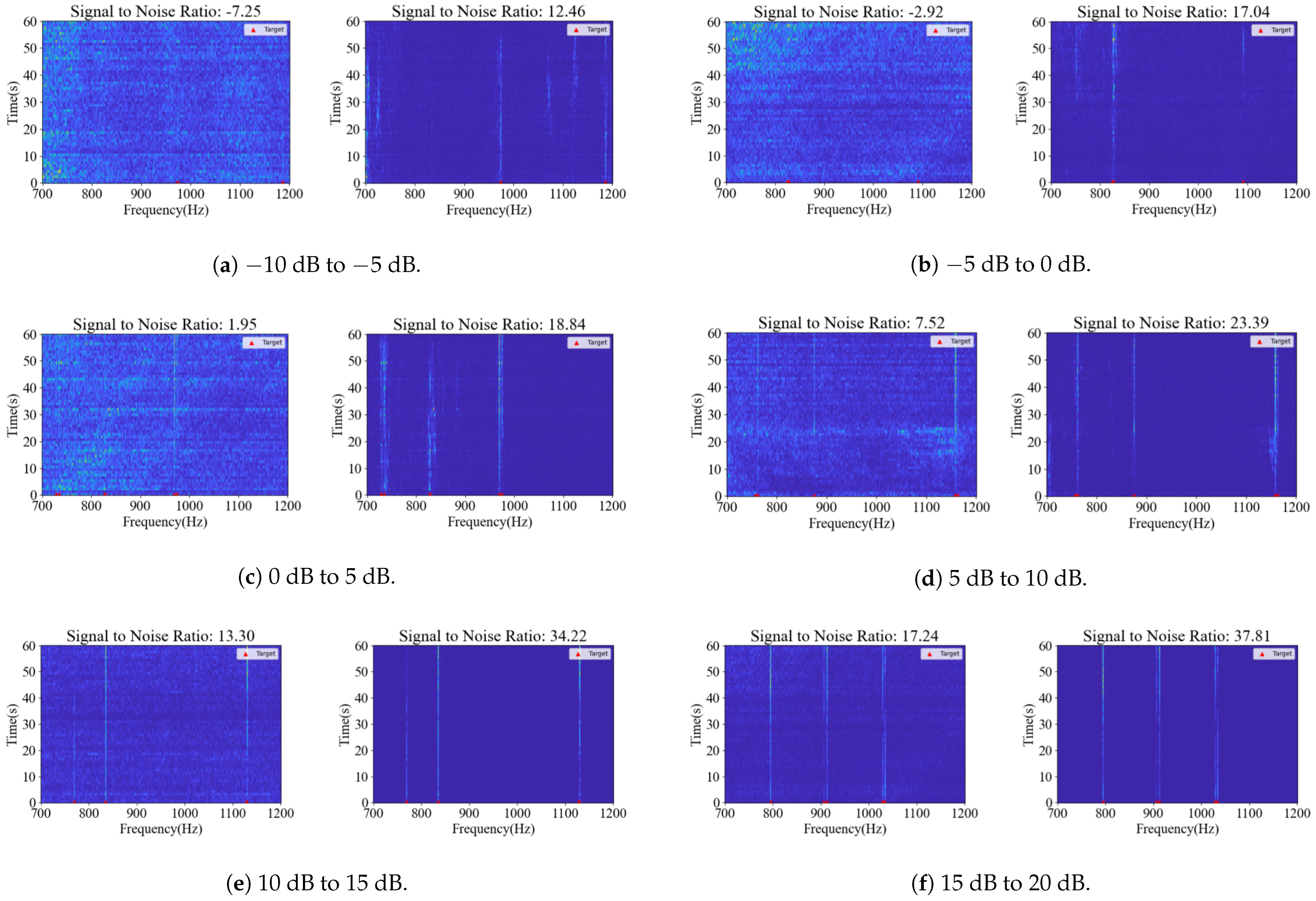
To quantify the line spectrum enhancement effect of the denoising method, signal-to-noise ratio (SNR) is used to measure the image quality of the LOFAR spectrogram, and the SNR gain evaluates the effectiveness of the convolutional denoising model proposed in this paper. For the set of pixels belonging to the collected LOFAR spectrogram $Y(T,F)$, denoted as $S\in {\mathbb{R}}^{(T\times F)}$, the set of pixels corresponding to the target signal is $S_t$, and the set of pixels corresponding to non-target signal is $S_n$, such that $S=S_t\cup S_n$ and $S_t\cap S_n=\varnothing$. In the calculation of SNR in Equation (6), since the powers of target signal and noise are not able to be calculated for real measured data, the average value of the non-target signal pixels is approximated as the noise signal power, while the difference between the average pixel value of the target signal region and the noise signal power is approximated as the target signal power. Therefore, the SNR based on the LOFAR spectrogram can be approximate by:

$$\mathrm{SNR}=10{log}_{10}\left({\displaystyle \frac{\frac{1}{|S_t|}{\sum }_{(t,f)\in S_t}{Y}^2(t,f)-\frac{1}{|S_n|}{\sum }_{(t,f)\in S_n}{Y}^2(t,f)}{\frac{1}{|S_n|}{\sum }_{(t,f)\in S_n}{Y}^2(t,f)}}\right)$$

(13)

The signal-to-noise ratio of model input is denoted as $SN{R}_{in}$ and the signal-to-noise ratio of model output is denoted as $SN{R}_{out}$. The signal-to-noise ratio gain G of the convolutional denoising model can be defined as:

$$G=SN{R}_{out}-SN{R}_{in}$$

(14)

In addition, the line spectrum recall is used as an evaluation metric for the model to determine whether the model suppresses the target line spectrum during the denoising process, which may lead to missed detections in subsequent analysis and recognition. It is defined as:

$$Recall=N_{correct}/N_{all}$$

(15)

where $N_{correct}$ represents the number of line spectrum peaks after denoising that match the true line spectrum frequencies, and $N_{all}$ represents the total number of true line spectrum. The true line spectrum frequencies are known conditions in the simulated data, while in the measured data, they are considered to be manually annotated. The two metrics exhibit a non-strict negative correlation. As the signal-to-noise ratio gain increases, the likelihood of suppressing the target line spectrum increases, while the likelihood of detection of line spectrum decreases. Therefore, both metrics are used together to evaluate the performance of proposed method.

4. Results

4.1. Comparison with Baselines

In this section, we evaluate the performance of our proposed convolutional denoising model(CDM) with two deep learning models: MSCU-net (multi-scale convolution U-Net) [20] and DPRNN (Dual-Path Recurrent Neural Network) [21]. These three models are trained on dataset A and tested on test set A1. However, MSCU-net is a two-dimensional model which treats the spectrogram of a noisy acoustic signal as input and the spectrogram of the clean acoustic signal as output. Thus, instead of using the soft threshold mask label for the target defined in Equation (9), the spectrogram of the clean acoustic signal is used as the label for model training, which is consistent with the training method described in the original paper. Additionally, DPRNN is a waveform-based model that directly denoises raw noisy acoustic signals, transforming them into clean signals, so the model directly uses the noisy one-dimensional acoustic signal as input and the clean one-dimensional acoustic signal as output for model training. The overall results are shown in

Table 1. Comparisons of different denoising methods on test set A1.

SNR Range	MSCU-Net [20]		DPRNN [21]		CDM (Ours)
	G	Recall	G	Recall	G	Recall
−10 dB to −5 db	0.8834	0.1853	3.9762	0.1676	10.7929	0.2294
−5 dB to 0 dB	2.6540	0.6563	8.7896	0.6347	18.0306	0.6780
0 dB to 5 dB	5.2922	0.8414	10.9292	0.8543	20.9799	0.9061
5 dB to 10 dB	9.3417	0.8423	13.6969	0.8825	21.0083	0.9631
10 dB to 15 dB	13.9782	0.8547	13.9269	0.8892	21.5888	0.9965
15 dB to 20 dB	18.1433	0.8571	16.3986	0.8362	21.7486	0.9965

.

For the simulation test set A1, the training and testing data come from the same marine area, the convolutional denoising model achieves a signal-to-noise ratio (SNR) gain of over 20 dB for underwater target signal with an SNR above 0 dB, and the recall rate of the line spectrum is greater than 90%. In extreme low SNR conditions, specifically between −10 dB and −5 dB, where the ocean noise power is significantly higher than target signal power, the convolutional denoising model still provides an SNR gain of 10.7929 dB. Although the recall rate of the line spectrum is only 22.94%. Under these extremely low SNR conditions, the convolutional denoising model is still able to extract some line spectrum that is completely masked in the original LOFAR spectrogram. Compared to MSCU-Net and DPRNN, our proposed convolutional denoising model outperforms both in terms of SNR gains and recall across all SNR levels, demonstrating significantly superior denoising performance. These results demonstrate that the model effectively suppresses noise while preserving the essential features of the original target signal to the greatest extent. One possible reason for the performance difference between the models is the variation in their training objectives. The convolutional denoising model focuses on separating the noisy signal into distinct noise and target components, while the other two models aim to directly transform the noisy signal into a clean one. This difference in approach may introduce unintended artifacts or overfitting, which could negatively impact their denoising effectiveness.

Furthermore, to verify the denoising effectiveness of the convolutional denoising model on real measurement data from the same marine area, using the same model as described above, tests are conducted on test dataset A2. The testing result is shown in

Table 2. Model performance metrics on test set A2.

${\mathit{SNR}}_{\mathbf{in}}$	${\mathit{SNR}}_{\mathbf{out}}$	G	${\mathit{N}}_{\mathbf{correct}}$	${\mathit{N}}_{\mathbf{all}}$	Recall
12.80 dB	30.10 dB	17.30	6	6	1

.

The results indicates effective noise reduction with gain G being 17.30, showing a substantial enhancement in signal quality. The recall of 1 demonstrates perfect identification of the target line spectrum in this dataset.

4.2. Model Transferability Validation

In practical applications, it is not possible to collect data at all times and all places for model training. Therefore, to verify the transferability and generalization on different marine areas, the aforementioned trained convolutional denoising model is tested on sea trial data B1. The testing result is shown in

Table 3. Model performance metrics on test dataset B1.

SNR range	G	${\mathit{N}}_{\mathbf{correct}}$	${\mathit{N}}_{\mathbf{all}}$	Recall
−10 dB to −5 dB	9.55	106	300	0.3533
−5 dB to 0 dB	14.68	244	323	0.7554
0 dB to 5 dB	16.65	265	280	0.9464
5 dB to 10 dB	17.71	276	278	0.9928
10 dB to 15 dB	19.62	293	294	0.9966
15 dB to 20 dB	21.16	249	249	1

.

The metrics of the deep convolutional denoising model on test dataset B1 are similar to those on test dataset A1. Although there is a slightly decrease in signal-to-noise ratio gain, the overall change is not significant. This indicates that the deep convolutional denoising model has a good transferability and generalization on different marine areas.The denoising effects for different signal-to-noise ratio ranges are shown in Figure 5, with the left image representing the raw LOFAR spectrogram and the right image representing denoised LOFAR spectrogram. The red arrows indicate the center frequencies of the simulated data.

To further verify the transferability and generalization of the convolutional denoising model on real measured data from different marine areas, the model is tested on test set B2. The result is shown in

Table 4. Model performance metrics on test set B2.

${\mathit{SNR}}_{\mathbf{in}}$	${\mathit{SNR}}_{\mathbf{out}}$	G	${\mathit{N}}_{\mathbf{correct}}$	${\mathit{N}}_{\mathbf{all}}$	Recall
11.15 dB	26.33 dB	15.18	189	213	0.8873

.

For the real measured data test set B2, the average signal-to-noise ratio of the underwater acoustic signal is 11.15 dB, while the average signal-to-noise ratio after denoising is 26.33 dB, resulting in an average signal-to-noise ratio gain of 15.18 dB and a recall rate of 88.73%. The metrics of the real measured data are quite similar to those of the simulation data, which not only demonstrates the transferability and generalization of the convolutional denoising model but also validates the practical application value of the proposed simulation-enhanced underwater acoustic signal LOFAR spectrogram denoising method.

4.3. Discussion and Analysis

This paper introduces an enhanced simulation algorithm designed to simulate target line spectrum features while integrating ocean noise. The primary objective of this algorithm is to generate a large volume of labeled data for model training. While previous studies have simulated data by mixing clean signals with noise, the performance of models can degrade where target data collection is challenging. To address this, we propose an enhanced simulation algorithm based on the assumptions that the pattern of line spectrum, such as the presence of Doppler effects, are known and if the simulated data closely resemble real data, they can be treated as realistic for model training purposes. A key feature of proposed enhanced simulation algorithm is the incorporation of the Doppler effect, which is particularly relevant for fast-moving vessels such as speedboats and unmanned underwater vehicles (UUVs). When direct data collection from a target is difficult and pattern of line spectrum is known, this algorithm can generate sufficient data for model training. Moreover, the pattern of the line spectrum does not necessarily indicate the type of target that must be known prior to model training. For instance, even for the same target, the inclusion or exclusion of the Doppler effect results in different line spectrum patterns.

The parameters in the enhanced simulation are crucial for ensuring the quality of the training samples. The signal duration T controls the length of the LOFAR spectrogram, with an empirical value set to 40, which has minimal impact on the quality of the simulated data. The lower frequency limit $f_l$ and upper frequency limit $f_h$ define the frequency range where the line spectrum appears. When mixed with ocean noise, it is important to ensure that the target frequency range remains clean, meaning that no unexpected line spectrum are present, as this could degrade the denoising model’s performance. The lower amplitude limit $A_l$ and upper amplitude limit $A_h$ control the prominence of the line spectrum. Higher values make the line spectrum more noticeable. Since it is difficult to denoise noisy data where the line spectrum is submerged in ocean noise, we aim for slightly weaker amplitude samples during the simulation, rather than higher amplitude samples, to better reflect complex conditions. The number of lines spectrum N varies across samples and depends on the frequency range of the spectrogram. A wider frequency range requires more line spectrum, as the ratio of line spectrum pixels to background pixels decreases, which introduces a significant pixel imbalance problem that can negatively affect the model’s denoising performance. The amplitude of frequency drift $f_d$ and amplitude drift $A_d$ introduce variability in the training samples and are tailored to the pattern of the line spectrum. For large vessels, such as cargo ships, the line spectrum is typically found in the low-frequency range, with minimal Doppler shifts due to their slower speeds. In contrast, for unmanned underwater vehicles (UUVs), significant frequency drift $f_d$ and amplitude drift $A_d$ must be applied to account for their higher speeds. If the underwater acoustic signal contains a rapidly moving vessel but the parameters $f_d$ and $A_d$ are not properly considered in the simulation, the denoising effect will deteriorate.

In this paper, two datasets, A and B, are introduced to evaluate the model’s generalization ability and transferability across different oceanic environments, where both simulation data and sea trail data are included. The ocean noise in these datasets is sourced from distinct locations, with synthetic data present in test sets A1 and B1, and real measured data in test sets A2 and B2. Compared to the ocean noise in dataset A, the noise in dataset B is more complex, featuring multiple vessels within the surrounding environment. The convolutional denoising model, which was trained using dataset A, is tested on both synthetic and real measured data to assess its performance in terms of generalization. This also serves to validate the hypothesis that, if simulated data closely resembles real-world conditions, it can be effectively used as input for model training. The results from test sets A1 and A2 reveal that when the signal-to-noise ratio (SNR) ranges between 10 dB and 15 dB, the model achieves an impressive SNR gain of 21.58 dB and a recall rate of 0.9965 in test set A1. These outcomes slightly outperform those obtained from the real measured data in test set A2, where the model achieves an SNR gain of 17.3 dB and a recall of 1. When the model, trained on dataset A, is directly tested on test sets B1 and B2, designed to evaluate its transferability, there is a slight reduction in both SNR gain and recall for both synthetic and real measured data. This suggests that while the model retains some degree of transferability to different ocean environments, its performance is somewhat reduced. This observed decrease is likely attributable to overfitting, as synthetic data typically contain fewer patterns compared to the more intricate and varied real measured data. A comparison between datasets A and B further confirms that the environment in dataset B is more complex, as evidenced by the slight decline in both SNR gain and recall. This difference aligns with the environmental conditions under which the data was collected. While the model demonstrates excellent generalization and transferability, the most effective approach of our method is to first collect ocean noise data from a well-defined marine environment. This data, combined with simulation algorithms, can then be used to create a large and diverse training dataset. Once trained, the model can be deployed in relevant scenarios. Therefore, It is highly recommended to deploy our denoising model in the same marine environment from which the ocean noise was collected, ensuring optimal performance. Moreover, additional validation across a broader range of conditions, including more extreme scenarios, is warranted to fully assess the model’s robustness and adaptability.

LOFAR and DEMON (Detection of Envelope Modulation on Noise) are crucial tools for analyzing, detecting, and recognizing targets. While denoising LOFAR spectrograms is an essential preliminary step, the ultimate goal is to detect and identify targets, and extract key attributes such as location, position, and the number of propeller blades. Moving forward, integrating advanced denoising techniques with detection, recognition, and other analytical methods will be a key focus of future research and development. Additionally, compared to directly reconstructing the denoised signal into the original signal, the proposed method can only be applied to LOFAR spectrogram analysis, which imposes limitations on its use. Future work should explore extending the method to more general signal reconstruction tasks beyond LOFAR spectrogram analysis.

5. Conclusions

5.1. Main Conclusion

This paper presents a LOFAR spectrograms denoising method for underwater acoustic signal based on enhanced simulation. A large amount of labeled sample data is generated through the simulation algorithm to train a convolutional denoising network model, which is then applied to denoise real measured data. Extensive simulations and experimental results demonstrate that the proposed method exhibits excellent noise suppression effects in real marine environments. Furthermore, the denoising model shows good transferability and generalization, as the trained model can adapt to different marine environments, laying the foundation for subsequent target feature analysis and target type recognition.

5.2. Limitations and Future Work

Although the proposed method demonstrates excellent transferability and generalization, it is essential to consider a broader range of environmental conditions. Future studies should focus on analyzing various pattern of line spectrum to enhance the simulation algorithms. Moreover, denoising serves as a foundational step for target detection and recognition, integrating denoising models with other detection and recognition systems to further improve recognition accuracy is also critical in future research.

References

1. Ali, M.F.; Jayakody, D.N.K.; Chursin, Y.A.; Affes, S.; Sonkin, D. Recent advances and future directions on underwater wireless communications. Arch. Comput. Methods Eng. 2020, 27, 1379–1412. [Google Scholar] [CrossRef]
2. Wang, P.; Peng, Y. Research on underwater acoustic target recognition based on LOFAR spectrogram and deep learning method. In Proceedings of the 2020 5th International Conference on Automation, Control and Robotics Engineering (CACRE), Dalian, China, 19–20 September 2020; pp. 666–670. [Google Scholar] [CrossRef]
3. Chen, J.; Han, B.; Ma, X.; Zhang, J. Underwater target recognition based on multi-decision LOFAR spectrogram enhancement: A deep-learning approach. Future Internet 2021, 13, 265. [Google Scholar] [CrossRef]
4. Lu, H.; Shang, J.; Chen, Y.; Ma, Q. A LOFAR spectrogram multi-sub-band matching method for passive target recognition. In Proceedings of the 2nd International Conference on Signal Image Processing and Communication (ICSIPC 2022), Qingdao, China, 20–22 May 2022; Volume 12246, pp. 139–150. [Google Scholar] [CrossRef]
5. Yao, H.; Gao, T.; Wang, Y.; Wang, H.; Chen, X. Mobile_ViT: Underwater Acoustic Target Recognition Method Based on Local–Global Feature Fusion. J. Mar. Sci. Eng. 2024, 12, 589. [Google Scholar] [CrossRef]
6. Yao, Q.; Wang, Y.; Yang, Y. Underwater Acoustic Target Recognition Based on Data Augmentation and Residual CNN. Electronics 2023, 12, 1206. [Google Scholar] [CrossRef]
7. Raj, K.M.; Murugan, S.S.; Natarajan, V.; Radha, S. Denoising algorithm using wavelet for underwater signal affected by wind driven ambient noise. In Proceedings of the 2011 International Conference on Recent Trends in Information Technology (ICRTIT), Chennai, India, 3–5 June 2011; pp. 943–946. [Google Scholar] [CrossRef]
8. Li, Y.-X.; Wang, L. A novel noise reduction technique for underwater acoustic signals based on complete ensemble empirical mode decomposition with adaptive noise, minimum mean square variance criterion and least mean square adaptive filter. Def. Technol. 2020, 16, 543–554. [Google Scholar] [CrossRef]
9. Hu, H.; Zhang, L.; Yan, H.; Bai, Y.; Wang, P. Denoising and baseline drift removal method of MEMS hydrophone signal based on VMD and wavelet threshold processing. IEEE Access 2019, 7, 59913–59922. [Google Scholar] [CrossRef]
10. Li, Y.-X.; Jiao, S.-B.; Gao, X. A novel signal feature extraction technology based on empirical wavelet transform and reverse dispersion entropy. Def. Technol. 2021, 17, 1625–1635. [Google Scholar] [CrossRef]
11. Ju, D.; Chi, C.; Li, Y.; Zhang, C.; Huang, H. A line spectrum Enhancement Algorithm Based on Unsupervised Deep Learning. Ship Sci. Technol. 2020, 42, 117–120. [Google Scholar] [CrossRef]
12. Yang, L.; Zhang, X.; Wu, B. Research on LOFAR spectrogram Enhancement of Passive Sonar Target signal Based on Long Short-Term Memory Networks. Electroacoust. Technol. 2020, 44, 101–103. [Google Scholar] [CrossRef]
13. Li, Y.; Ma, X.; Wang, L.; Liu, Y. Denoising and Reconstruction of Pulsed signal in Non-Gaussian Environments Based on Deep Learning. Appl. Acoust. 2021, 40, 142–146. [Google Scholar] [CrossRef]
14. Yin, J.; Luo, W.; Li, L.; Han, X.; Guo, L.; Wang, J. Enhancement of Underwater Acoustic Signal Based on Denoising Autoencoder. J. Commun. 2019, 40, 119–126. [Google Scholar] [CrossRef]
15. Cao, L.; Peng, Y.; Mu, L.; Sun, Y.; Xu, J. A Water Sound Signal Recognition Method Based on Deep Convolutional Networks and Convolutional Denoising Autoencoders. Cyber Secur. Data Gov. 2023, 42, 35–3845. [Google Scholar] [CrossRef]
16. Luo, W. Research on Sonar Signal Feature Enhancement Technology Based on Deep Learning. Master’s Thesis, Harbin Engineering University, Harbin, China, 2020. [Google Scholar] [CrossRef]
17. Jiang, Y. Research on Recognition and Separation of Underwater Acoustic signal Based on Generative Adversarial Networks. Master’s Thesis, Harbin Engineering University, Harbin, China, 2021. [Google Scholar] [CrossRef]
18. Gu, T.; Zhang, Q.; Li, J. Study on spectrogram Line Enhancement of Underwater Targets Based on Time-Frequency Attention Mechanism Network. J. Electron. Inf. 2024, 46, 92. [Google Scholar] [CrossRef]
19. Ronneberger, O.; Fischer, P.; Brox, T. U-Net: Convolutional Networks for Biomedical Image Segmentation. In Proceedings of the Medical Image Computing and Computer-Assisted Intervention (MICCAI 2015), Munich, Germany, 5–9 October 2015; Springer: Berlin/Heidelberg, Germany, 2015; pp. 234–241. [Google Scholar]
20. Ma, T.; Yan, S.; Wang, W. An underwater acoustic signal denoising algorithm based on U-Net. In Proceedings of the 2023 IEEE International Conference on Signal Processing, Communications and Computing (ICSPCC), Zhengzhou, China, 14–17 November 2023; pp. 1–6. [Google Scholar] [CrossRef]
21. Song, Y.; Liu, F.; Shen, T. A novel noise reduction technique for underwater acoustic signals based on dual-path recurrent neural network. IET Commun. 2023, 17, 135–144. [Google Scholar] [CrossRef]
Figure 1. Framework of the LOFAR spectrogram denoising method for underwater acoustic signal based on enhanced simulation.
Applsci 14 10931 g001
Figure 2. The structure of convolutional denoising model.
Applsci 14 10931 g002
Figure 3. Training samples.
Applsci 14 10931 g003
Figure 4. Real measurement data.
Applsci 14 10931 g004
Figure 5. Different signal-to-noise ratio ranges of raw LOFAR spectrogram and denoised LOFAR spectrogram.
Applsci 14 10931 g005