An Integrated Model for Dam Break Flood Including Reservoir Area, Breach Evolution, and Downstream Flood Propagation

Abstract

The reasonable and efficient prediction of dam failure events is of great significance to the emergency rescue operations and the reduction in dam failure losses. This work presents a model that is based on the physical mechanism. It is coupled with a multi-architecture (multi-CPU and GPU) open-source two-dimensional flood model, which is based on high-precision terrain and land use data. The aim is to enhance the accuracy of dam break flood process simulations. The model uses DEM data as a computational grid and updates it at each time step to reflect breach evolution. Simultaneously, the breach evolution model incorporates an analysis of stress on sediment particles, establishing the initial erosion state and lateral expansion model while accounting for seepage. The determination of the overflow of the breach is resolved through the application of a two-dimensional hydrodynamic model. This approach achieves a robust connection between the upstream reservoir, the dam structure, and the downstream inundation area. The coupled model is utilized to calculate the failure of earth-rock dams and landslide dams, and a sensitivity analysis is conducted. Taum Sauk Dam and Tangjiashan landslide dam were selected to represent earth dam break and barrier lake break, respectively, which are the main types of dam breaks. The obtained results demonstrate strong concurrence with the measured data, the relative errors of the four important parameters of the application case, the peak discharge of the breach, the top width of the final breach, the depth of the breach and the arrival time of the maximum peak discharge are all within ±10%. Although the relative error of the completion time of the final breach is greater than 10%, it is about 30% less than the relative error of the physical model.

1. Introduction

Reservoirs and dams were constructed on rivers to effectively harness and utilize water resources for the purposes of flood control, agriculture, power generation, and water supply. Reservoirs and dams significantly contributed to the advancement of society and the economy. However, they also provide significant potential hazards due to their large water storage capacity. In the case of a dam breach, it will surely pose a substantial threat to the areas downstream [1]. A dam breach is a rare but highly perilous event that can result in immediate and immensely devastating floods, posing significant economic and social consequences for nearby and downstream regions. In recent years, due to climatic change and intensified human activities, there has been a notable increase in the frequency and intensity of extreme climate events [2]. Consequently, the ability of reservoirs and dams to effectively regulate floods is being challenged by increasingly severe conditions. To mitigate the damage caused by dam break disasters, a mathematical model is employed to simulate the occurrence of dam break accidents. This model serves as a dependable foundation for predicting the progression of dam break floods, determining the extent of risk, and evaluating the repercussions of the disaster.

The primary objective of the dam break flood simulation research is to study the development process of the breach and the routing of the resulting flood. Parameter models or mechanism models are employed to simulate the progression of breach formation [3,4]. The parameter models are derived from past dam break statistical data and employ regression analysis or machine learning to construct empirical formulas. These formulas enable the estimation of dam break parameters such as peak flow, final size of the breach, and length of the dam break event [5]. Currently, the parameter models that are often utilized include the SCS model from the Soil and Water Conservation Centre of the United States [6], the Macdonald model [7], the American Bureau of Agricultural Reclamation model [8], the Von Thun and Gillete model [9], the Froehlich model [10,11], the Xu and Zhanga model [12], and the Zhong Qiming dam break parameter model [13]. Furthermore, due to the proliferation of dam break databases, the precision of parameter models is steadily improving. However, these models also have certain limitations. One limitation is their excessive dependence on the dam break database, while another limitation is their inability to capture the flow process and development of the dam break. The mechanism model is a mathematical representation created by considering the physical process of a breach. It typically takes into account factors such as flow depth, shear stress, and dam material parameters to forecast the breach’s features and the resulting outflow. The model typically comprises the continuity equation, the sediment and water motion equation, and auxiliary equations that account for the beginning conditions and boundary conditions. In the BEED model developed by Singh et al., erosion was determined using the Einstein–Brown bedload formula [14]. The peak discharge of the dam break flood and the time it took for the breach to form aligned closely with the observed values. However, the calculated values at the top of the breach differed significantly from the observed values. The NWS BREACH model, developed by Fread, utilizes the modified Meyer–Peter Müller formula to accurately compute the erosion process [15]. This model is specifically designed for analyzing the overtopping or piping failure of earth dams and clay core dams. The NWS BREACH model is included into the hydrodynamic model MIKE, which was developed by the Danish Hydraulic Institute. However, the accuracy of this model is low, and it significantly deviates from important experimental results. The HR BREACH model categorizes the dam break process into five distinct stages. Each stage utilizes specific erosion formulas, and a technique is introduced to determine the shape of the breach by calculating the effective shear stress [16,17], and the accuracy is greatly affected by the case characteristics. The WinDAM model, jointly developed by the USDA Agricultural Research Service (ARS), Natural Resources Conservation Service (NRCS), and Kansas State University, employs the dam erosion formula and the slope movement formula to precisely estimate erosion. However, it does not incorporate the factor of lateral collapse [18]. The DL Breach model, created by WU Weiming, utilizes both non-viscous and viscous erosion equations to accurately compute the erosion process. It also considers the displacement of steep ridges, allowing for the simulation of dam failure resulting from overtopping and piping. The peak flow and the extent of the breach correspond closely to the observed values. However, the model assumes that the rate of lateral expansion is proportional to the rate of vertical erosion [19]. The NHRI-DB model developed by the Nanjing Institute of Hydraulic Science uses the erosion rate formula based on shear stress principles to compute both the vertical erosion and lateral development of a breach [20]. It also takes into account the downslope headward erosion, allowing for an accurate simulation of the downslope tanking process. Although this model utilizes the linear shear stress equation published by Graf (1984) [21] to determine the rate at which the bed erodes, it is important to note that this approach may result in an overestimation of the breach. The DB-IWHR model, developed by CHEN, utilizes the simplified Bishop method to calculate breach development [22]. It introduces a hyperbolic formula to account for erosion along the depth, effectively preventing transitional erosion. The model achieves a good simulation effect by incorporating water velocity as a step in the calculation. The mechanism model considers the physical mechanism of dam break development, which is more in line with reality. However, each model also has its limitations, mainly in that it mostly adopts the sediment transport formula based on the test data of river sediment transport, or it does not fully consider the development process of the collapse, such as defining the horizontal expansion process and the vertical development process as a simple linear relationship, or the collapse in the process of collapse development is not considered.

For the simulation of flood propagation process, the commonly used hydrodynamic models usually include a one-dimensional model, two-dimensional model, and three-dimensional model [23,24,25]. A one-dimensional river model has been widely used because of its flexibility and high computational efficiency [26]. For example, the HEC-RAS model developed by the US Army Corps of Engineers (USACE) [27] and the MIKE model are coupled with the one-dimensional hydrodynamic model [28]. Zhang Dawei et al. developed a one-dimensional dam break flood analysis system based on geographic information system for calculating the risk of dam break flood [29]. However, a dam break flood is usually not limited to one-dimensional river channels, but usually breaks out of the river channels and floods into the downstream plain area, which has obvious two-dimensional characteristics, so the two-dimensional model is more applicable [30]. The more famous two-dimensional hydrodynamic business models include the Telemac-2D model developed by Électricité de France (EDF) [31], MIKE21 model and HEC-RAS 2D model [32], and InfoWorks ICM model developed by Innovyze Company in UK.

At present, the simulation of dam break flood mostly adopts the segmented method of calculating the evolution of the breach and the flood propagation process, respectively; that is, firstly, the development process of the breach is calculated by using the parameter model or the mechanism model to obtain the flow process of the breach, and then the result is used as the input of the flood evolution model. However, the process of dam break is a process involving the hydraulic power of the upstream reservoir area, the evolution of the breach, and the flood propagation in the downstream inundation area. The reduction in reservoir water level, the development of the breach, and the flood propagation process in the downstream area are carried out simultaneously, and they affect each other. The level of local water level before the breach directly affects the development of the breach, the development of the breach determines the discharge volume, and the breach discharge determines the difference of the downstream inundation situation. The dam break process is more consistent with the real process by solving the dam break process and downstream flood propagation in the same time step. Based on this, Hu Xiaozhang [33] established a mathematical model, which adopted a one-dimensional model in the upstream reservoir area, a two-dimensional hydrodynamic model in the downstream inundation area, and adopt weir formula to connect the dam breach. However, in this model, the breach process was relatively simple, and the soil dynamics of the evolution of the collapse were not considered. Ma Liping [34] used the source term method to establish a coupling model which included the two-dimensional hydrodynamic process of the upstream reservoir, the one-dimensional evolution of the breach, and the two-dimensional propagation of the flood in the downstream inundation area, but the traditional weir flow formula was used to calculate the flow of the breach. At the same time, the two-dimensional propagation of dam break flood generally has a long distance, a large range, and a high dependence on terrain. The high-precision terrain can make the simulation results more accurate but will lead to an increase in calculation. Bladé [35] developed a two-dimensional hydrodynamic model, IBER, which coupled the evolution of a breach and the propagation of a flood. IBER can be calculated by CPU or GPU with high performance. However, the breach evolution module includes two types, one can be defined by users, and the other follows the specifications of the Spanish Technical Guide [36] of the parameter model, and the physical mechanism is poor. Xu Dong et al. realized large-scale flood evolution simulation through the cluster computing technology based on message passing interface (MPI) [37]. Hou Jingming developed a two-dimensional hydrodynamic model based on GPU parallel acceleration technology [38]. Parallel computing and the use of HPC on new architectures of modern supercomputers have become fundamental requirements for studying hydrodynamic problems at large spatial scales and high temporal resolution. However, in the high-performance hydrodynamic models of these coupled dam break models, the calculation of the outflow is mostly based on the weir flow formula, or the physical mechanism of the breach development is not fully considered. Therefore, although physics-based breach development models developed rapidly, it is still necessary to improve the models, and to better match the real breach process, it is necessary to solve the dam failure process and downstream flood evolution in the same time step.

This paper incorporates the seepage impact based on stress analysis of soil particles, and a novel horizontal expansion mechanism is proposed. Simultaneously, the dam break model is integrated with the two-dimensional hydrodynamic model utilizing multi-GPU acceleration technology. This integration establishes a high-performance two-dimensional flood propagation coupling model that encompasses the upstream reservoir, breach evolution, and downstream inundation area. The simulation and sensitivity analysis of Taum Sauk Dam and Tangjiashan landslide dam demonstrate that the coupled model is reliability, applicability, and efficiency.

2. Materials and Methods

2.1. Hydrodynamic Model

2.1.1. Governing Equation

This research utilizes the multi-architecture (multi-CPU and GPU) open-source two-dimensional flood model, known as TRITON, developed by Oak Ridge Laboratory of the United States [39]. The model is based on the analysis of the source term full shallow water equation and is used to simulate the spread of dam break floods. The grid utilized in this model is a Cartesian square grid derived straight from the DEM file, eliminating the need for constructing a dedicated computing grid.

In this paper, the two-dimensional shallow water equation is used to simulate the propagation process of dam break flood, and its vector form is as follows:

$${\displaystyle \frac{\partial \mathit{U}}{\partial t}}+{\displaystyle \frac{\partial \mathit{F}}{\partial x}}+{\displaystyle \frac{\partial \mathit{G}}{\partial y}}={\mathit{S}}_{\mathit{r}}+{\mathit{S}}_{\mathit{b}}+{\mathit{S}}_{\mathit{f}}$$

$$\mathit{U}=\left(\begin{array}{c}h\\ q_x\\ q_y\end{array}\right)\mathit{F}=\left(\begin{array}{c}{q}_x\\ {\displaystyle \frac{q_x^2}{h}}+{\displaystyle \frac{1}{2}}g{h}^2\\ {\displaystyle \frac{q_x{q}_y}{h}}\end{array}\right)\mathit{G}=\left(\begin{array}{c}{q}_y\\ {\displaystyle \frac{q_x{q}_y}{h}}\\ {\displaystyle \frac{q_y^2}{h}}+{\displaystyle \frac{1}{2}}g{h}^2\end{array}\right)$$

(1)

$${\mathit{S}}_{\mathit{r}}=\left(\begin{array}{c}r\\ 0\\ 0\end{array}\right){\mathit{S}}_{\mathit{b}}=\left(\begin{array}{c}0\\ -gh{\displaystyle \frac{\partial z}{\partial x}}\\ -gh{\displaystyle \frac{\partial z}{\partial y}}\end{array}\right){\mathit{S}}_{\mathit{f}}=\left(\begin{array}{c}0\\ -{\displaystyle \frac{g{n}^2}{h^{7/3}}}{q}_x\sqrt{q_x^2+q_y^2}\\ -{\displaystyle \frac{g{n}^2}{h^{7/3}}}{q}_y\sqrt{q_x^2+q_y^2}\end{array}\right).$$

In the formula, $\mathit{U}$ is a variable vector, including water depth $h$, discharge per unit width $q_x$, and $q_y$ in the $x$ and $y$ directions; $g$ is the gravitational acceleration; $r$ is runoff rate; $n$ is Manning roughness coefficient; and $\mathit{F}$ and $\mathit{G}$ are flux vectors in the $x$ and $y$ directions, respectively. S_r is the runoff source term. ${\mathit{S}}_{\mathit{b}}$ is the source term of the bed slope. ${\mathit{S}}_{\mathit{f}}$ is the friction source term. $z$ is the elevation of the bed.

2.1.2. Numerical Method

The integrated coupling model is implemented on the basis of the 2D hydrodynamic model TRITON. The TRITON model employs a numerical approach to solve the two-dimensional shallow water equation (Equation (1)) on a square Cartesian grid with grid spacing $∆x$. This is accomplished using a finite-volume method with an upwind strategy. The grid cell interface fluxes are computed by employing an approximate Riemannian solver that incorporates an upgraded Roe method. The average approximate solution method of Echeverribar et al. [40], was employed to handle the flux and bottom slope source terms of each edge grid. This approach effectively prevents negative water depth values without the need to decrease the time step, thereby ensuring the accuracy of the solution. The friction source term employs local implicitness to enhance stability, while the CFL number is utilized to regulate the time step. The numerical method efficiently resolves the calculation instability and the nonconservation of material momentum resulting from unrealistic physical phenomena, such as negative water depth and artificially high flow velocity at the dry–wet interface of complex terrain. Additionally, it can effectively address flow issues under diverse conditions. Simultaneously, the model uses CUDA programming language to provide parallel computing technology, enabling the transition from a single CPU and GPU to numerous ones, hence achieving high-speed operation.

2.2. Breach Evolution Model

The breach development model used in this paper is a new developed conceptual lumped model with physical significance. It consists of five primary modules: breach flow calculation, initiation of scour at the breach, vertical erosion of the breach, lateral expansion of the breach, and stability analysis of the breach slope. Unlike the majority of models, this particular model takes into account the impact of seepage effect on the critical velocity by analyzing the stress of soil particles. It then derives the formula for lateral erosion of the slope in the breach and builds a model for lateral expansion.

2.2.1. Breach Flow Calculation

The flow of the breach is influenced by various intricate aspects, including the inflow of water from upstream, the storage capacity of the reservoir, the features of the breach section, and the water depth near the breach. The general dam break model involves computing the variation in reservoir storage capacity during each time interval based on the inflow of water from upstream and the reservoir’s capacity curve. The weir formula is employed to compute the discharge of the breach, whereas the Manning formula is utilized to determine the water level of the breach [20,33,34]. The proposed integrated model in this research calculates the water depth and flow velocity by updating the terrain at each time step and solving the two-dimensional shallow water equation. Moreover, the hydraulic parameters, such as breach discharge and water depth, can be obtained, thereby circumventing the inaccuracies resulting from calculation methods such as the average water depth of the reservoir, the weir flow formula, and the Manning formula. This ultimately improves the accuracy of the breach discharge calculation.

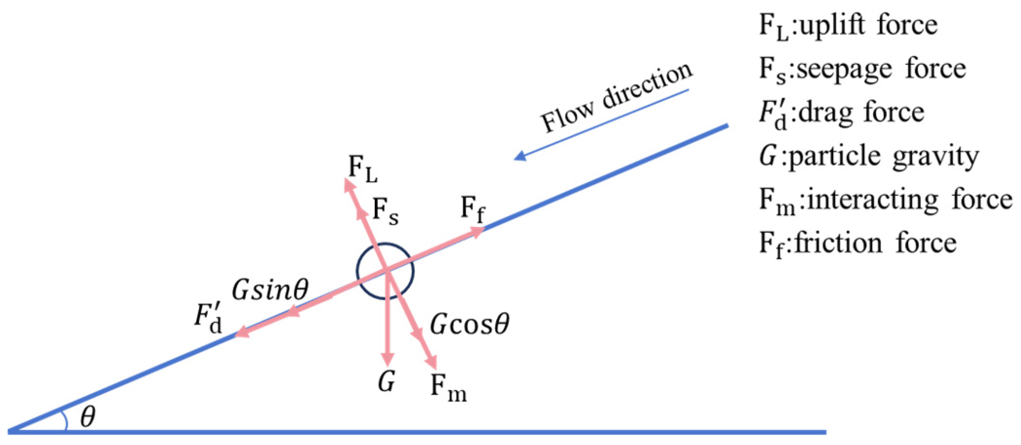
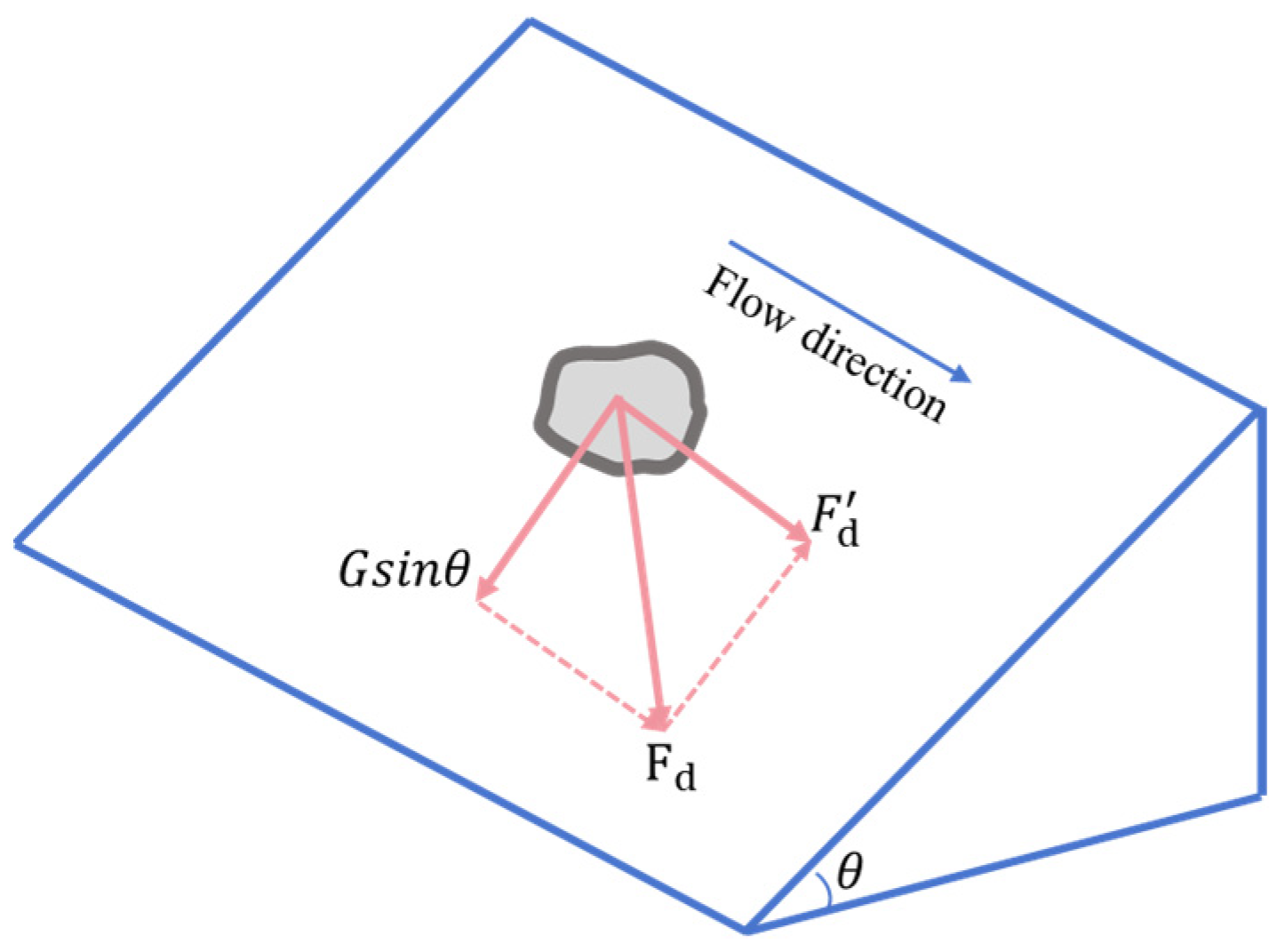
2.2.2. Starting Erosion Condition of the Breach

The critical flow velocity formula, with and without seepage force, is derived by analyzing the force of a soil particle on the slope. The forces acting on a soil particle on the dam slope mainly include the soil particle gravity $\mathit{G}$, the drag force ${\mathit{F}}_{\mathit{d}}^{\mathit{\prime }}$, the uplift force ${\mathit{F}}_{\mathit{L}}$ exerted by water flows, the interacting force ${\mathit{F}}_{\mathit{m}}$, the friction force ${\mathit{F}}_{\mathit{f}}$, and the seepage force ${\mathit{F}}_{\mathit{s}}$. The force analysis is shown in Figure 1.

The particle gravity of the soil particle is expressed as follows [41]:

$$\mathit{G}={\displaystyle \frac{1}{6}}({\gamma }_s-{\gamma }_w)\pi D^3,$$

(2)

where ${\gamma }_s$ is the specific weight of the soil particle, ${\gamma }_w$ is the water weight; $D$ is the diameter of the soil particle, represented by D₅₀, the median particle size of the non-uniform mixed sediment.

The uplift force calculation formula is as follows [42]:

$${\mathit{F}}_{\mathit{L}}=C_L{\displaystyle \frac{\pi D^2}{4}}{\displaystyle \frac{\rho v^2}{2}}={\displaystyle \frac{\pi }{80g}}{\gamma }_w{V}^2{D}^2,$$

(3)

where $C_L$ is the coefficient of the uplift force and is usually equal to 0.1; $\mathit{g}$ is the acceleration due to gravity, $\rho$ is the density of water; and $V$ is the velocity of flow.

The drag force calculation formula is written as follows [42]:

$${\mathit{F}}_{\mathit{d}}^{\mathbf{\prime }}=C_D{\displaystyle \frac{\pi D^2}{4}}{\displaystyle \frac{\rho v^2}{2}}={\displaystyle \frac{\pi }{20g}}{\gamma }_w{V}^2{D}^2,$$

(4)

where $C_D$ is the coefficient of the drag force and usually takes the value of 0.4.

The seepage force calculation formula is written as follows [43]:

$${\mathit{F}}_{\mathit{s}}={\displaystyle \frac{\pi }{6(1-e)}}i{\gamma }_w{D}^3,$$

(5)

where $i=\mathsf{\Delta }H/L$, $\mathsf{\Delta }H$ is the difference of water level elevation between two points of the water level line, that is, the difference of water level between the unit before the dam and the unit behind the dam. $L$ is the horizontal distance between these two points, which is the width of the dam; e is the porosity of the dam material.

The interacting force calculation formula is written as follows [44]:

$${\mathit{F}}_{\mathit{m}}=1.5M({\gamma }_s-{\gamma }_w)D^3,$$

(6)

$$M=0.75-{\displaystyle \frac{0.65}{2+C_u}},$$

(7)

where $C_u$ is the non-uniformity coefficient.

According to the force analysis of the soil particles, it could be concluded that the friction force of the soil particle at its incipience when seepage force is considered can be written as follows:

$${\mathit{F}}_{\mathit{f}}=tan\phi (\mathit{G}cos\theta +{\mathit{F}}_{\mathit{m}}-{\mathit{F}}_{\mathit{L}}-{\mathit{F}}_{\mathit{s}}).$$

(8)

when seepage force is not considered, the friction force is:

$${\mathit{F}}_{\mathit{f}}=tan\phi (\mathit{G}cos\theta +{\mathit{F}}_{\mathit{m}}-{\mathit{F}}_{\mathit{L}}),$$

(9)

where $\phi$ is the internal friction angle of soil material, $\theta$ is the inclination of dam slope. The analysis of the forces acting on the soil particle reveal that the critical condition for incipient motion is as follows:

$${\mathit{F}}_{\mathit{d}}^{\mathbf{\prime }}+\mathit{G}sin\theta ={\mathit{F}}_{\mathit{f}}.$$

(10)

Substituting Equations (3)–(6) and (8) into (10), the starting flow velocity considering seepage flow is obtained as follows:

$${\mathit{V}}_{\mathit{c}}=\sqrt{{\displaystyle \frac{120gtan\phi M({\gamma }_s-{\gamma }_w)D}{\pi {\gamma }_w(4+tan\phi )}}+{\displaystyle \frac{40g(tan\phi cos\theta -sin\theta )({\gamma }_s-{\gamma }_w)D}{3{\gamma }_w(4+tan\phi )}}-{\displaystyle \frac{40\pi giDtan\phi }{3(1-e)(4+tan\phi )}}}.$$

(11)

Substituting Equations (3)–(6) and (9) into (10), the starting flow velocity without considering seepage flow is obtained as follows:

$${\mathit{V}}_{\mathit{c}}=\sqrt{{\displaystyle \frac{120gtan\phi M({\gamma }_s-{\gamma }_w)D}{\pi {\gamma }_w(4+tan\phi )}}+{\displaystyle \frac{40g(tan\phi cos\theta -sin\theta )({\gamma }_s-{\gamma }_w)D}{3{\gamma }_w(4+tan\phi )}}}.$$

(12)

2.2.3. Breach Vertical Erosion Module

When the flow velocity at the breach is greater than the critical starting velocity, the breach erosion begins. The vertical erosion process of the breach is the hyperbolic model proposed by Chen Zuyu [22,45], whose expression is as follows:

$${\displaystyle \frac{∆Z_b}{∆t}}={\displaystyle \frac{\nu }{a+b(\tau -{\tau }_c)}}\ast {10}^{-3},$$

(13)

where the shear stress $\nu =k(\tau -{\tau }_c)$ after deducting the critical shear stress, $k$ is the unit transformation factor allowing $∆Z_b/∆t$ to approach its extreme value within the range of shear stress $\tau$, and k is taken as 100 here, and ${\tau }_c$ is the critical shear stress. $a$ and $b$ are the parameters of the hyperbolic model, and the reference values of the parameters can be found in the literature [46]. The hyperbolic model has an asymptote $1/b$ as $\nu$ approaches infinity, which represents the maximum possible erosion rate of the soil. $1/a$ denotes the slope of the curve for $\nu =0$.

The shear stress $\tau$ and the critical shear stress ${\tau }_c$ are calculated using the following formula [47]:

$$\tau ={\gamma }_{w}RJ\approx {\displaystyle \frac{{\gamma }_w{n}^2{V}^2}{{Z_b}^{1/3}}},$$

(14)

$$V=\sqrt{{\mathit{u}}_{\mathit{x}}^2+{\mathit{u}}_{\mathit{y}}^2},$$

(15)

$${\tau }_c={\displaystyle \frac{2}{3}}D({\gamma }_s-{\gamma }_w)tan\phi ,$$

(16)

where $n$ is the roughness coefficient; $R$ is the hydraulic radius, $J$ is the hydraulic gradient, $Z_b$ is the water depth in the breach, $V$ is the flow velocity of breach section, and ${\mathit{u}}_{\mathit{x}}$ and ${\mathit{u}}_{\mathit{y}}$ are the velocities in the $x$ and $y$ directions, respectively.

2.2.4. Breach Lateral Evolution Module

Under the lateral erosion of the outburst flood, the dam breach will become wider. It is currently assumed in most models that the lateral erosion rate is twice that of the vertical erosion rate during the dam break [48,49]. A linear extension model for calculating the lateral development of the breach is provided, while the initial movement conditions of sediment particles and the difference in slope are ignored. Therefore, the simulated lateral erosion of the breach does not fully match the actual situation. In order to solve this problem, a method is proposed for calculating the width of the breach by deducing the lateral evolution formula through the theoretical analysis of the initial movement of sediment in the dam slope. The forces acting on sediment particles in the slope mainly include particle gravity component $\mathit{G}sin\theta$, the combined drag force ${\mathit{F}}_{\mathit{d}}$, and the critical drag force ${\mathit{F}}_{\mathit{d}}^{\mathit{\prime }}$, as shown in Figure 2.

The combined drag force of dragging ${\mathit{F}}_{\mathit{d}}$ on the side slope of breach and the underwater gravity along the slope is calculated as follows:

$${\mathit{F}}_{\mathit{d}}=\sqrt{{\left(\mathit{G}sin\theta \right)}^2+{{\mathit{F}}_{\mathit{d}}^{\mathbf{\prime }}}^2}.$$

(17)

The initial motion condition of sediment particles on the breach side slope:

$$\sqrt{{\left(\mathit{G}sin\theta \right)}^2+{{\mathit{F}}_{\mathit{d}}^{\mathbf{\prime }}}^2}=tan\phi (\mathit{G}cos\theta -{\mathit{F}}_{\mathit{L}}-{\mathit{F}}_{\mathit{s}}).$$

(18)

From the Equation (18), the critical drag force ${\mathit{F}}_{\mathit{d}}^{\mathit{\prime }}$ of sediment particles on the breach side slope can be expressed as the following:

$${\mathit{F}}_{\mathit{d}}^{\mathbf{\prime }}=\sqrt{{tan}^2\phi {(\mathit{G}cos\theta -{\mathit{F}}_{\mathit{L}}-{\mathit{F}}_{\mathit{s}})}^2-{\left(\mathit{G}sin\theta \right)}^2}.$$

(19)

The change rate of sediment erosion ${\displaystyle \frac{∆E_r}{∆t}}$ on the breach side slope is calculated as the following:

$${\displaystyle \frac{∆E_r}{∆t}}={\displaystyle \frac{\sqrt{{tan}^2\phi {(\mathit{G}cos\theta -{\mathit{F}}_{\mathit{L}}-{\mathit{F}}_{\mathit{s}})}^2-{\left(\mathit{G}sin\theta \right)}^2}}{\frac{\pi D^2}{4}·\rho }}.$$

(20)

The initial sediment erosion rate $E_s$ on the breach side slop can be expressed by:

$$E_s={\displaystyle \frac{∆E_r}{∆t}}·{\tau }_c={\displaystyle \frac{\sqrt{{tan}^2\phi {(\mathit{G}cos\theta -{\mathit{F}}_{\mathit{L}}-{\mathit{F}}_{\mathit{s}})}^2-{\left(\mathit{G}sin\theta \right)}^2}}{\frac{\pi D^2}{4}·\rho }}·{\tau }_c.$$

(21)

In the scouring process of dam break, the erosion rate of the breach side slope varies with shear stress $\tau$ of the water flow. Thus, the actual widened erosion area per unit time $E_b$ can be simulated by the following formula [50]:

$$E_b={\displaystyle \frac{E_s}{{\gamma }_s}}·{\displaystyle \frac{\tau -{\tau }_c}{{\tau }_c}},$$

(22)

substituting Equations (21) into (22):

$$E_b={\displaystyle \frac{\sqrt{{tan}^2\phi {\left(\mathit{G}cos\theta -{\mathit{F}}_{\mathit{L}}-{\mathit{F}}_{\mathit{s}}\right)}^2-{\left(\mathit{G}sin\theta \right)}^2}}{\frac{\pi D^2}{4}·\rho ·{\gamma }_s}}\left({\tau -\tau }_c\right).$$

(23)

The increase in breach bottom width within the time step is expressed as:

$$\mathsf{\Delta }{B}_i={\displaystyle \frac{C_b·E_b·\mathsf{\Delta }\mathrm{t}}{L}},$$

(24)

substituting Equations (23) into (24):

$$\mathsf{\Delta }{B}_i={\displaystyle \frac{4C_b\sqrt{{tan}^2\phi {\left(\mathit{G}cos\theta -{\mathit{F}}_{\mathit{L}}-{\mathit{F}}_{\mathit{s}}\right)}^2-{\left(\mathit{G}sin\theta \right)}^2}}{\pi D^2·\rho ·{\gamma }_s·L}}({{\tau }_i-\tau }_c)\mathsf{\Delta }t,$$

(25)

where $L$ is the length of flow chute, $C_b$ is the coefficient of side slope, if only one side is eroded, $C_b$ equals to 1.0. For a breach with erosion of both sides $C_b$ equals 2.0.

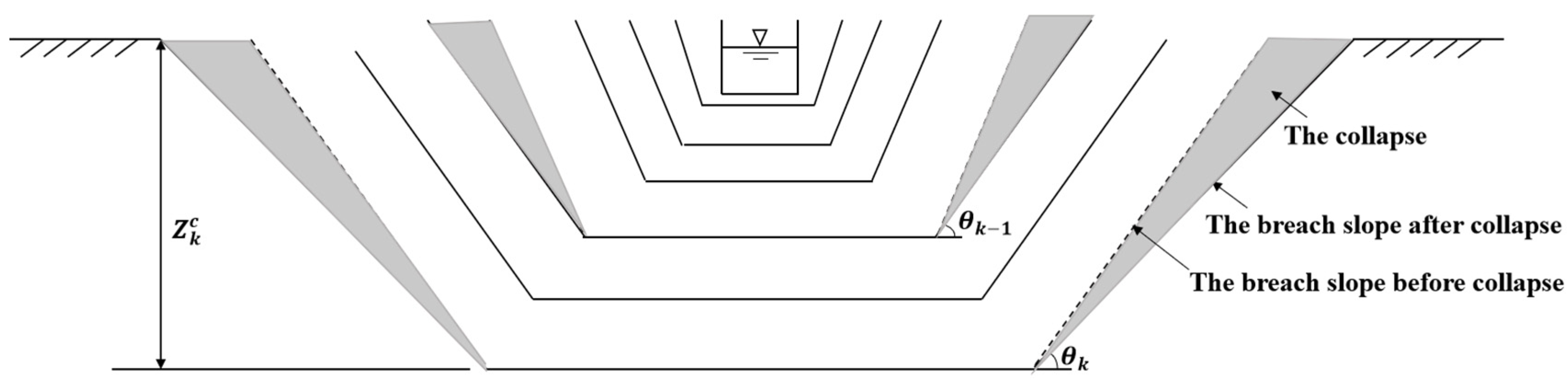
2.2.5. Side Slope Stability Module

With the development of vertical erosion of the breach, the breach slope gradually deepened and the slope angle gradually increased. When the anti-sliding force on the sliding surface of the slope is not enough to resist the sliding force of the sediment, the sediment in the upper part of the slope will be displaced along the sliding surface and lose its original stability, leading to collapse. In this model, the initial breach is assumed to be rectangular, and gradually becomes trapezoidal as the breach expands. When the vertical depth of the breach reaches the critical water depth, the breach slope will collapse due to instability. Figure 3 shows a schematic diagram of the collapse and expansion process of the dam breach slope.

The critical depth $Z_k^c$ can be deduced by the limit equilibrium method, and the formula is as follows [51]:

$$Z_k^c={\displaystyle \frac{4ccos\phi sin{\theta }_{k-1}}{{\gamma }_s[1-\mathrm{c}\mathrm{o}\mathrm{s}({\theta }_{k-1}-\phi \left)\right]}},k=\mathrm{1,2},3\dots ,$$

(26)

where $Z_k^c$ is the critical depth, $c$ is cohesion, $\phi$ is the internal friction angle of soil material; ${\theta }_{k-1},{\theta }_k$ are the angle of the dam site at different times.

The initial breach is rectangular, that is, ${\theta }_0=\pi /2$. The slope of the collapse is calculated as follows:

$${\theta }_k={\displaystyle \frac{1}{2}}({\theta }_{k-1}+\phi ).$$

(27)

The final average width of the breach is controlled by the actual value or the empirical formula [52], which is as follows:

$$B_m=0.1803K{V}_r^{0.32}{Z}_k^{0.19},$$

(28)

where $B_m$ is the average width of the final breach, $Z_k$ is the final depth of the breach, $V_r$ is the effective discharge capacity of the reservoir corresponding to the final breach depth, and $K$ is the correction coefficient, which is set to be 1.0 for the breach caused by overtopping and 1.4 for the breach caused by piping.

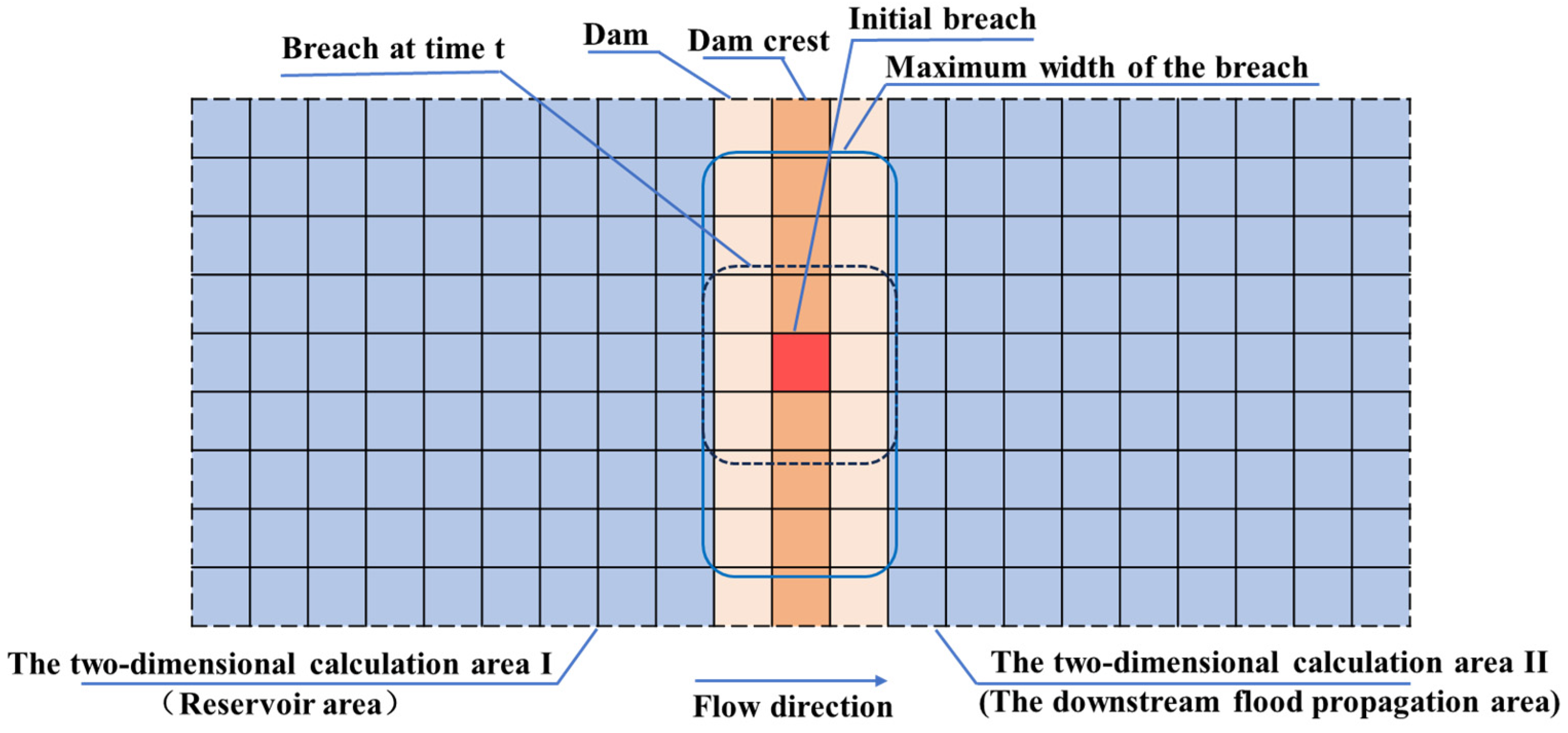
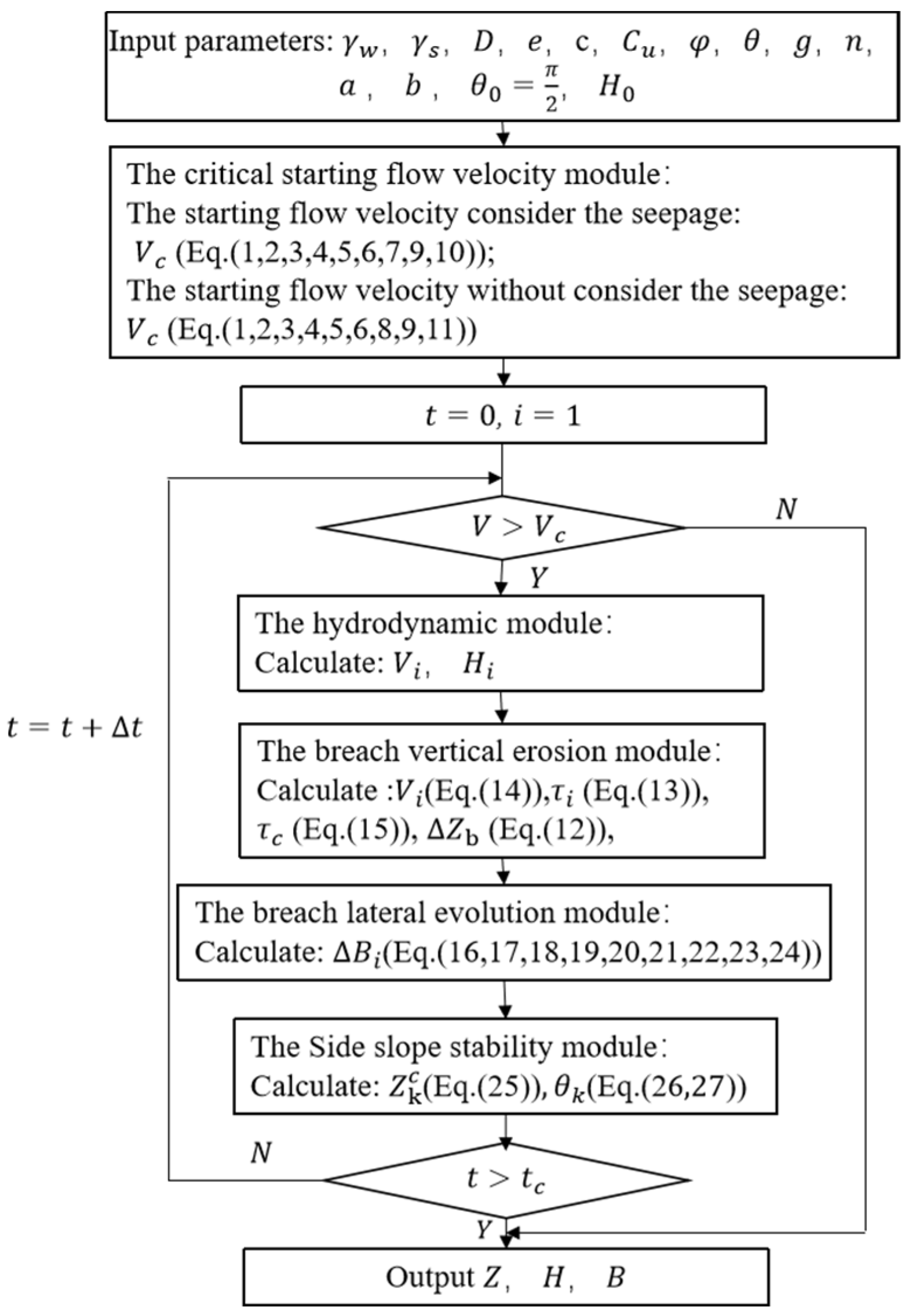
2.3. Integrated Model Construction

The most important data of this model are the terrain data (digital elevation model, DEM), and the grid used for the model calculation is the structural grid obtained directly from the DEM. The advantage of the model is that no preprocessing step is required to generate the computational grid, which improves the running efficiency of the model. The DEM data used in this integrated model include the underwater topography of the reservoir area, the elevation of the dam, and the terrain of the downstream inundation area.

Figure 4 shows the schematic diagram of the integrated simulation. As shown in Figure 4, the orange grid is the dam area, the red grid is the initial breach, the two-dimensional calculation area I is the upstream reservoir area, and the underwater terrain of the reservoir area is used, and the two-dimensional calculation area II is the downstream flood propagation area. The location of the dam and the initial breach are located according to the latitude and longitude. The DEM value in each time step is updated according to the scour depth of the breach, and then the water depth and current velocity value of each grid are updated through the flood propagation model. The new water depth and current velocity values at the breach grid are used to calculate the breach evolution model in the next time step.

Figure 5 shows the flow chart of the model. The most important feature of this coupled model is that the iteration of each time step is realized by directly updating the DEM of the computational grid, and the regional grid of the dam is involved in the model calculation instead of only describing the shape of the dam. The driving water depth and current velocity values of the breach evolution are directly calculated by the corresponding water depth and current velocity values of the breach at the previous time step. This avoids the process of using the weir flow formula to calculate the flow out of the breach. At the same time, through the water depth in each time step rather than using the reservoir capacity curve to reflect the changes in the water volume of the reservoir area, the strong coupling of the upstream reservoir area, the dam, and the downstream propagation area is realized.

The coupled models input data by writing files in a specific format and output the result data in a specific format. The necessary input data of the model are configuration file and terrain file (DEM). Additional data include roughness coefficient, source boundary information, streamflow hydrograph, runoff hydrograph, etc. The roughness can be provided either as a constant number or in the form of a matrix raster map matching the number of DEM grid cells. The output of the model includes water depth and unit discharge data. Two types of output data (spatial and temporal) are generated in a separate folder, each user-specified: one is that the water depth and unit discharge are written in the form of a matrix type file, and the other is that the water depth and unit discharge at the specified point locations (defined in the input files) can be output in a single file for each variable. The resulting data can be post-processed and displayed by a variety of tools, which provides great flexibility.

2.4. Comparison

In this part, the method proposed in this paper is compared with the existing physical mechanism model method to highlight the innovation of this paper. To calculate the breach outburst flow, existing models usually use the weir formula. However, the integrative model is proposed in this paper, the water depth and flow velocity of the previous time are used to drive the evolution of the outburst in the next time step, and then the flow of the breach is calculated. In the judgement of initial erosion, existing models are mostly based on the flow velocity or shear stress. In this paper, the critical flow velocity formula, with and without seepage force, is derived by analyzing the force of a soil particle on the slope. To calculate the breach lateral evolution, existing models are mostly assumed in a linear relationship between the lateral expansion and vertical erosion of the breach. In this paper, the lateral evolution formula is derived from the theoretical analysis of the initial sediment movement in the dam slope. At the same time, the breach side slope stability module is considered in this paper, which is not considered in some existing models. The comparison between the integration model and other common simplified physical models is shown in

Table 1. The comparison between the integration model and existing models.

No.	Models	Breach Flow Calculation	Breach Vertical Erosion	Breach Lateral Evolution	Breach Side Slope Stability
1	DAMBRK [53]	Weir formula	Assumed linear erosion	Linearly related to vertical erosion	No consider breach stability
2	HR BREACH [16]	Variable weir plus 1D steady nonuniform equation	Various equations, noncohesive and cohesive soils	Linearly related to vertical erosion	Consider breach stability
3	WinDAM [18]	Weir formula	Headcut advance, bottom and lateral erosion	Linearly related to vertical erosion	No consider breach stability
4	MIKE DB [28]	Weir formula	Engelund-Hansen bed load formula	Linearly related to vertical erosion	Consider breach stability
5	DLBreach [19]	Weir formula	Exponential erosion model	Linearly related to vertical erosion	Consider breach stability
6	DB-IWHR [22]	Weir formula	The hyperbolic erosion model	Linearly related to vertical erosion	Consider breach stability
7	NHRI-DB [20]	Weir formula	Exponential erosion model	Linearly related to vertical erosion	Consider breach stability
8	Integration model	Direct calculation by integration model	The hyperbolic erosion model	Newly proposed	Consider breach stability

.

2.5. Case Study

In order to verify the accuracy and performance of the integrated model, the Taum Sauk dam and Tangjiashan landslide dam were selected as the research cases in this paper. These two cases belong to the gradual dam break of overtopping. The gradual overtopping dam break includes the earth dam break and barrier lake break, which are the main types of dam breaks. The input parameters related to dam characteristics and soil properties of the integrated model are shown in

Table 2. Information of the Taum Sauk and the Tangjiashan landslide dams.

Basic Information	Taum Sauk Dam	Tangjiashan Landslide Dams
Location	90°49′6″ E, 37°32′8″ N	104°25′57″ E, 31°50′40″ N
Volume (m3)	5.366 × 106	2.3 × 107
Dam crest elevation (m)	487.38	742.5
Dam bottom elevation (m)	455.37	639.5
Dam height (m)	32.01	103
Dam crest width (m)	3.7	300
Dam breach bottom elevation (m)	456	717.5
Final breach depth (m)	31.38	25
Upstream slope ratio (vertical/horizontal)	1:1.3	1:1.5
Downstream slope ratio (vertical/horizontal)	1:1.3	1:1.5
Initial breach width (m)	10	8
Initial breach depth (m)	2	13
Average particle size (m)	0.01	0.03
$\mathrm{Porosity}e$	0.46	0.4
Average density of dam material (kg/m3)	2.65 × 103	2.6 × 103
Internal friction angle (°)	38	45
Cohesive force (kPa)	20	60
Erosion parameter	a = 1.0, b = 0.0005	a = 1.1, b = 0.0007

.

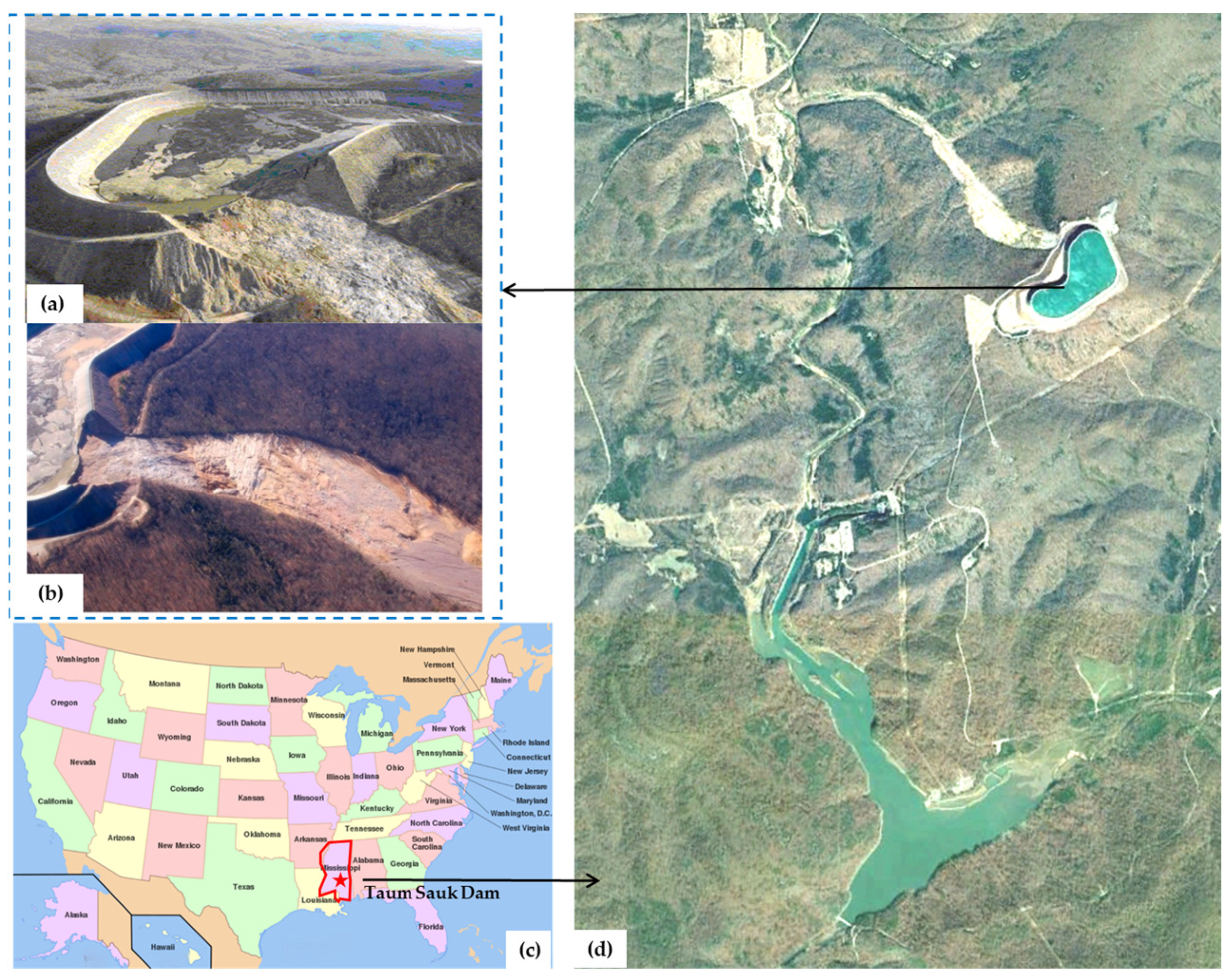
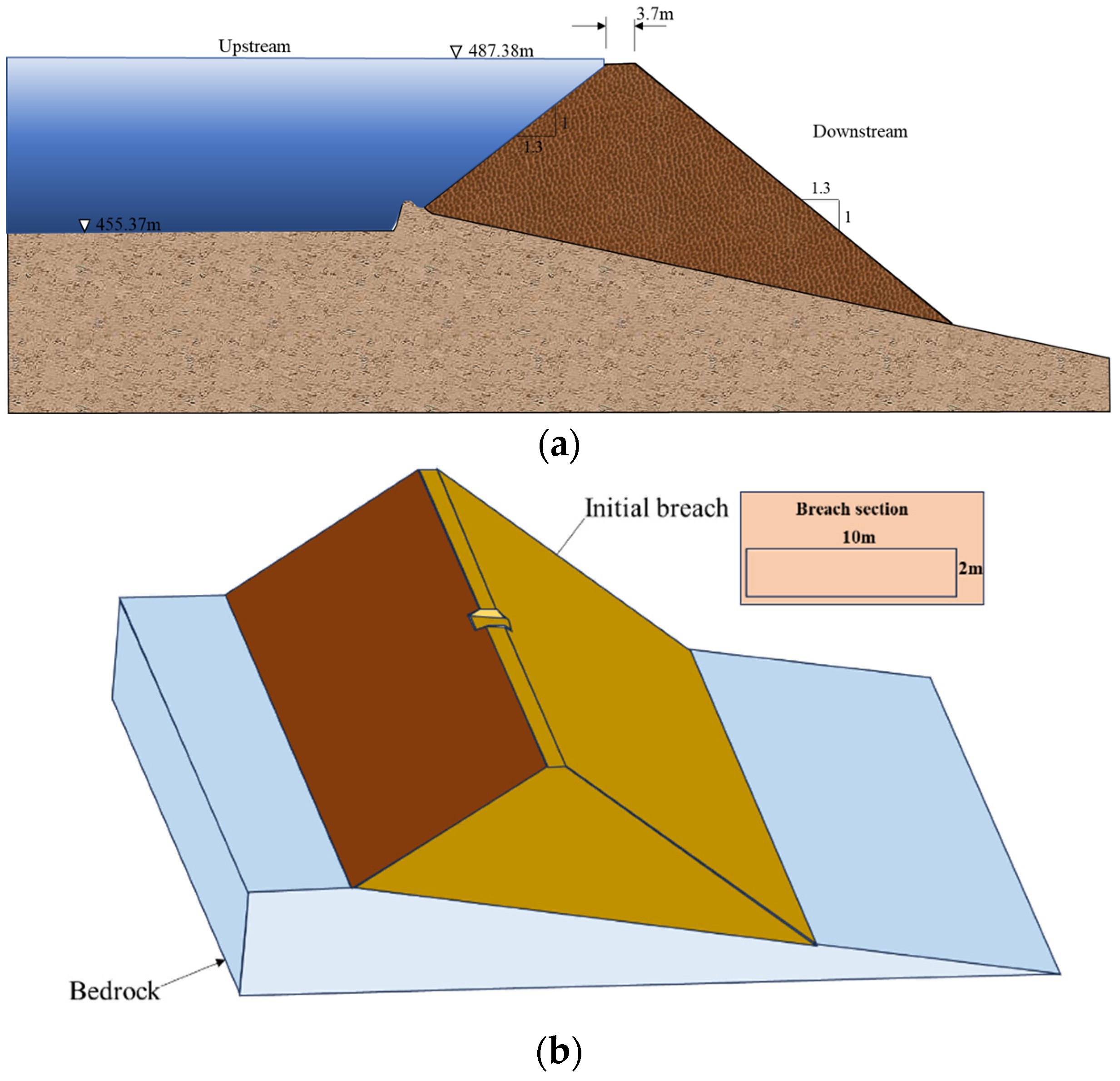
2.5.1. Taum Sauk Dam

The study object is the upper reservoir of the Taum Sauk Pumped Storage Power Station in Reynolds County, Missouri State, United States. The project was completed in 1962 and put into operation in 1963. On 14 December 2005, the stage sensors of the upper reservoir failed to turn off the pumps employed to convey water from the lower reservoir during the overnight filling, resulting in the water overflowing the wall top of Upper Taum Sauk dam. When the dam breached, 5.30 million m³ of water was released within 25 min and flowed into the Black River. After the dam break occurred, the US Geological Survey (USGS), the local natural resources department, and many flood research institutions conducted investigations on the accident and obtained detailed data on the dam break [54]. At the same time, the Oak Ridge Laboratory in the United States was developing a multi-architecture (multi-CPU and GPU) open-source two-dimensional flood model based on the source term full shallow water equation analysis (TRITON), and in this model, Taum Sauk is simulated as a typical case [39,55]. The hydrograph in TRITON is from the USGS analysis of the event [56], in which the discharge is developed from a volume analysis of the reservoir and knowledge of the embankment failure. The location of Taum Sauk dam and the shape of the breach are shown in Figure 6.

The terrain for this study is a 9.36 m USGS DEM covering the 62 km² extent of the flood event with 708,864 model grid cells (624 × 1136). The instability area of the dam is selected, and the initial position of the breach is determined. The initial breach is 10 m wide and 2 m deep in the middle of the dam, and the final breach width is 274 m. The profile of the dam is shown in Figure 7.

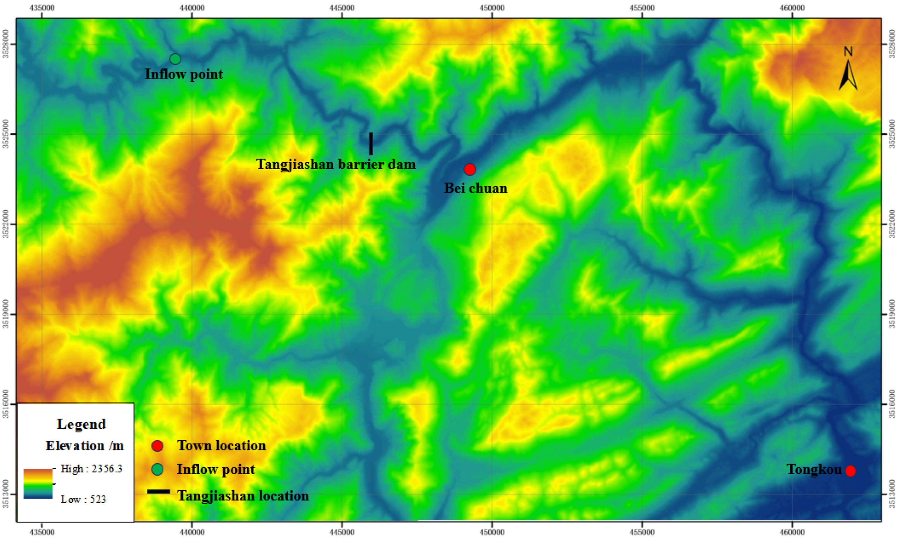
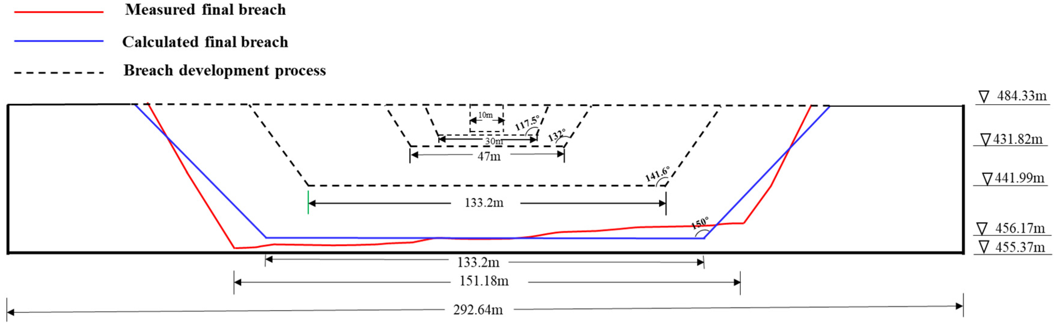
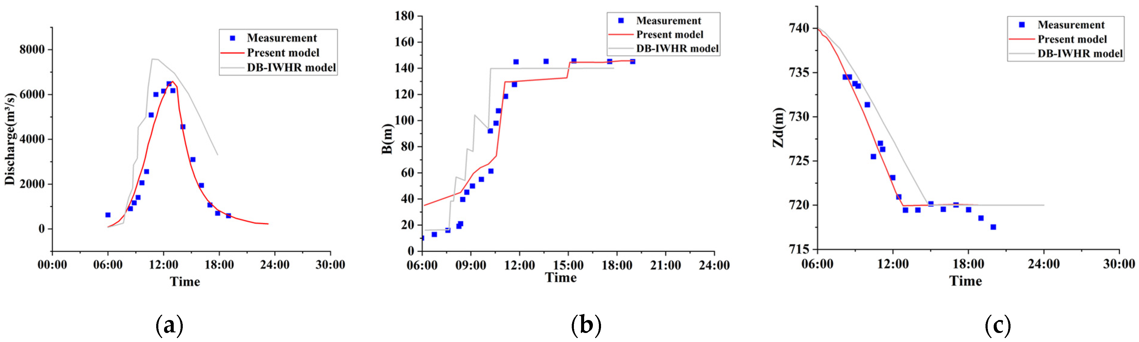
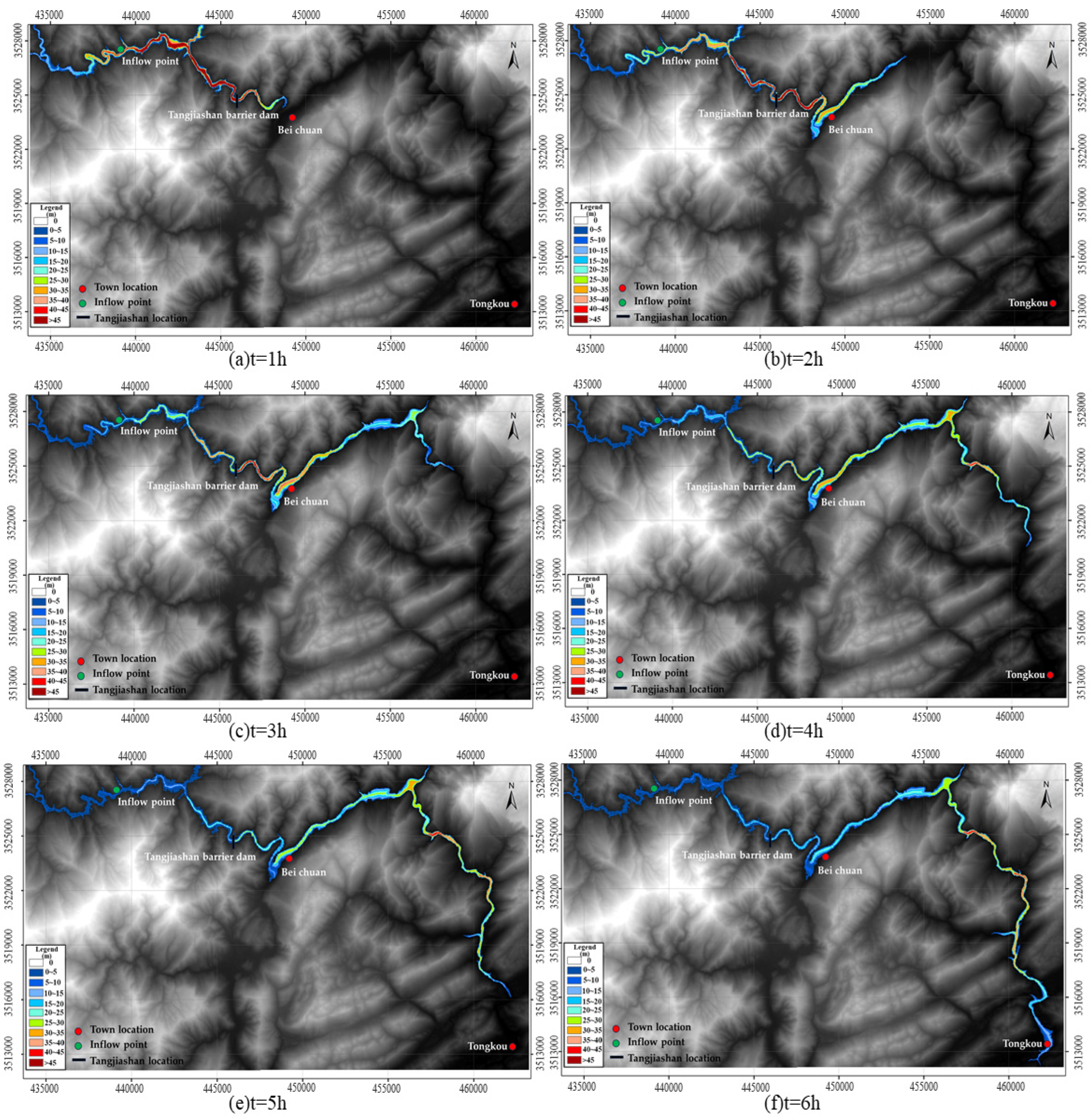
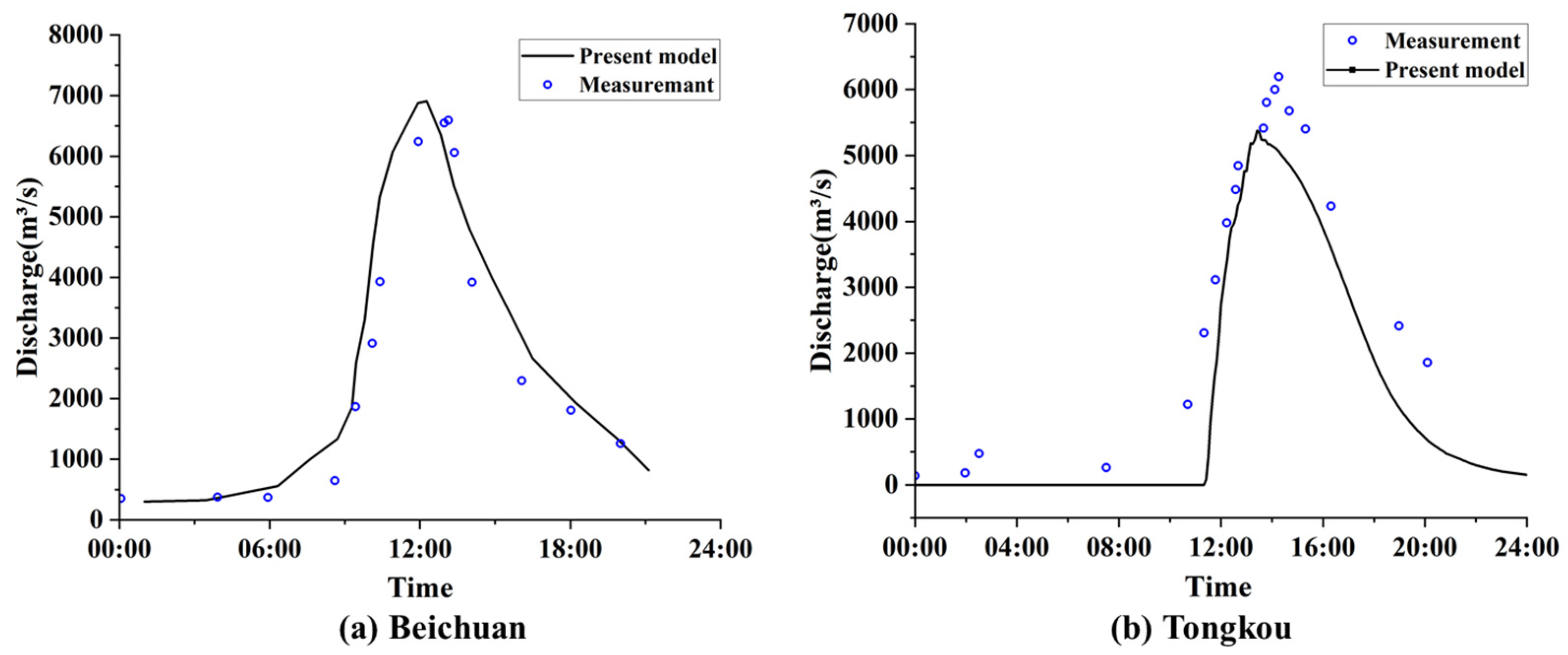
2.5.2. Tangjiashan Landslide Dam

On 12 May 2008, a seismic event with a magnitude of 8.0 occurred in Wenchuan County, located in the southwestern part of Sichuan Province. This event triggered a landslide in Tangjiashan, resulting in the obstruction of a river and the formation of a barrier lake. The Tangjiashan Barrier Lake experienced a breach at 6:00 on 10 June 2008, as the water level hit 742.5 m and the reservoir capacity surpassed 230 million m³ [20]. This work focuses on simulating the flow processes of the breach and the hydrodynamic process of the upstream and downstream areas inside a rectangular area extending 20 km upstream and 33 km downstream from the barrier dam. The terrain’s digital elevation model (DEM) has a resolution of 30 m, as shown in Figure 8. The downstream border represents the unrestricted flow out of the system, while the other limits are closed, meaning they do not allow any flow. The simulation lasts for a duration of 20 h, and there are a total of 793,000 grids. The failure of the Tangjiashan barrier dam resulted in an incomplete breach of the dam. At a height of 69 m above the dam’s base, the progress of the breach is halted due to the presence of substantial rocks within the dam, obstructing the further deepening of the breach. Hence, the longitudinal incision of the fracture terminates at a height of 69 m above the base of the dam in this computation. Simultaneously, during the risk mitigation process, a discharge channel in the shape of an inverted trapezoid has been excavated on the right dam shoulder of the Tangjiashan dam. The channel has a bottom width of 8 m, a depth of 13 m, and a side slope ratio of 1:1.5 (vertical/horizontal). This channel is intended to assist in safe discharge. To accurately replicate the discharge process, the model selects the unidirectional erosion development mode. To simplify the calculation and analysis of the irregularly shaped Tangjiashan Barrier Lake, we assume that it can be represented by trapezoids in both the horizontal and vertical directions. The dam has a height of 103 m and a top width of 300 m. The initial breach has a width of 8 m and a depth of 13 m. The model parameters are determined based on Zhong’s parameters [57,58,59], while the input data pertaining to dam features and soil conditions are presented in Table 2.

3. Results and Discussion

3.1. Results Analysis

The erosion resulting from water flowing through the discharge channel widens the break, while the initial discharge is minimal. As the breach becomes bigger, the amount of discharge gradually increases. Simultaneously, the outlet’s erosion capacity contributes to the swift enlargement of the breach. When the breach’s depth reaches a critical threshold, the breach slope collapses due to instability, promptly causing further expansion of the breach and accelerating the evolution process.

The Taum Sauk dam break is selected as an example in this paper. Firstly, the vertical comparison with the TRITON is used to verify the influence of the integrated model after adding the breach evolution module on the simulation accuracy of the dam break flood. Secondly, it is compared with the measured data and physical models DLBreach to verify the accuracy and efficiency of the newly proposed physics-based integrated model.

Table 3. The comparison of main parameters results of the Taum Sauk dam breach.

Parameter	Measured Data	Distributed Simulation Results	Relative Error	Integration Model Results	Relative Error	DLBreach	Relative Error
$Q_p$ (m3/s)	8180	9362.7	21.11%	8300	7.37%	8398.7	2.67%
$B_f$ (m)	199.95	——	——	210.7	5.38%	130.00	25.96%
$D_f$ (m)	28.16	——	——	28.16	0.00%	28.4	0.85%
$T_p$ (s)	480	360	−25.00%	502	4.58%	780	62.5%
$T_b$ (min)	25	——	——	32	28.00%	40	60.0%

summarized and compared the observed values and simulated values of the five important parameters of the Taum Sauk dam break event, including the peak discharge of the breach ($Q_p$), the top width of the final breach ($B_f$), the depth of the breach ($D_f$), the arrival time of the maximum peak discharge ($T_p$), and the completion time of the final breach ($T_b$). Figure 9 shows the results of the breach flow processes of different models. It can be seen that the integration model has the best fit with the measured data, the peak discharge simulated by the TRITON distributed model is larger, and the arrival time of the maximum peak discharge simulated by the DLBreach model is delayed.

As shown in Table 3, among the five important parameters, the relative errors of the other four parameters are within ±10%, except for the dam break completion time ($T_b$), which has a large relative error. The simulation accuracy of the peaking flow of the integrated model is higher than that of the distributed model, and the arrival time of the peaking flow is better than that of other models.

Figure 10 shows the measured shape of the final breach after the Taum Sauk dam failure and the calculated breach development by the integrated simulation model. As shown in Table 3 and Figure 10, the length and shape of the final breach calculated by the simulation model fit the actual breach well, and the relative error of the top width of the final breach is 5.38%. The formation time of the final breach simulated by the integrated model is 32 min, which is 6 min longer than the actual formation time, and the relative error is 28.00%. The relative error is within the acceptable range, indicating that the integrated model is acceptable.

The Tangjiashan landslide dam is selected as another example in this paper. The performance of the integrated model was assessed by comparing and analyzing the simulation results of breach discharge, breach breadth, and breach bottom elevation with both the actual data and the simulation results of DB-IWHR [22].

Figure 11 displays the discharge of water flowing out of the breach, as well as the variations in the width and bottom elevation of the breach. The integrated model is capable of accurately representing the discharge process of the breach and the changes in breadth and bottom elevation of the breach. When comparing the DB-IWHR model and actual data, the integrated model demonstrates superior ability to accurately mimic the regression process of the flow, as shown in Figure 11a. The integrated model has the capability to accurately replicate the abrupt expansion of the breach breadth resulting from the instability of the wedge, as depicted in Figure 11b, and the variation in the breach bottom elevation fits well with the actual data, as shown in Figure 11c.

As shown in Figure 12: the water depth map of the upstream and downstream areas at various time points during the dam failure. This map clearly illustrates the progression of the flood in the downstream area, the decrease in water level in the upstream reservoir, and the steady reduction in the flooded area.

The discharge process measured at the downstream Beichuan and Tongkou locations was chosen for comparison with the simulation findings of the coupling model. Among these, the distance between the Beichuan and the barrier dam is 7 km, while the Tongkou is located 33.5 km away from the barrier dam. Figure 13 illustrates that the flood arrival time at Beicuan is 1 h ahead of the actual time, and the peak discharge of the breach is 315 m³/s (4.78%) higher than the measured value. The flood discharge process at the Tongkou dam is accurately represented during the rising stage. However, the peak discharge is lower than the reported value of 594 m³/s (10.61%). Additionally, the flood flow is generally lower during the falling stage. The primary cause of the inaccuracy is that during the initial phase of the dam break, the simulated discharge process exceeds the measured discharge process. This results in an accelerated rise in discharge and an increase in the peak discharge at Beichuan. The discrepancy between the discharge attenuation rate observed in the simulation results and the measured discharge attenuation rate is primarily due to the precision of the topography data. The simulation of the Tangjiashan Barrier Lake break event demonstrates that the integrated model accurately replicates the peaking discharge, breach width, bottom elevation, flood propagation, and typical section discharge process. This indicates that the model is effective in simulating the dam break event of the Tangjiashan Barrier Lake.

3.2. Sensitivity Analysis

To assess the stability of the model, a sensitivity analysis is conducted using data from the Tangjiashan Barrier Lake. This involves changing one influencing parameter at a time while keeping the others constant and evaluating the impact of the main parameters in each module on the breach’s development and discharge.

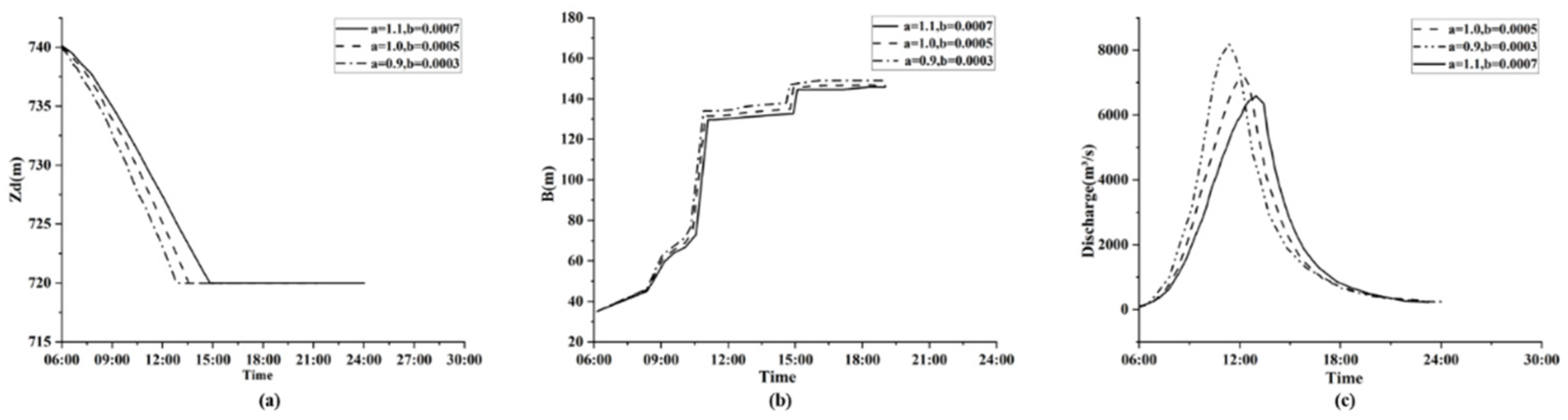
3.2.1. Influence of the Parameter Related to the Erosion Module

The parameters a and b of the hyperbolic erosion model have a direct impact on the pace at which the breach bottom erodes vertically. These parameters are crucial in the downcutting process of the breach bottom. The hyperbolic model uses parameters a and b with values of 1.1 and 0.0007, respectively. In the comparison case, parameters a and b have values of 1.0 and 0.0005, and 0.9 and 0.0003, respectively. These values reflect two soils that are more susceptible to erosion. They are used to assess the effect on the breach development caused by the outflows.

As shown in Figure 14a, it displays the breach bottom elevation for various erodibility parameters. The rate of vertical erosion increases as the values of parameters a and b decrease. However, the eventual height of the bottom of the breach remains unaffected by the values of a and b. As shown in Figure 14b, as the soil erodes further, the eventual breach becomes bigger. As shown in Figure 14c, the maximum discharge of the breach is significantly influenced by the parameters a and b. As the parameters a and b decrease, the discharge curve of the breach becomes steeper. This is primarily because the soil is more susceptible to erosion with lower values of a and b. Consequently, the vertical erosion rate of the breach and the enlargement speed of the lateral breach are accelerated, leading to a larger peaking discharge and an earlier appearance time.

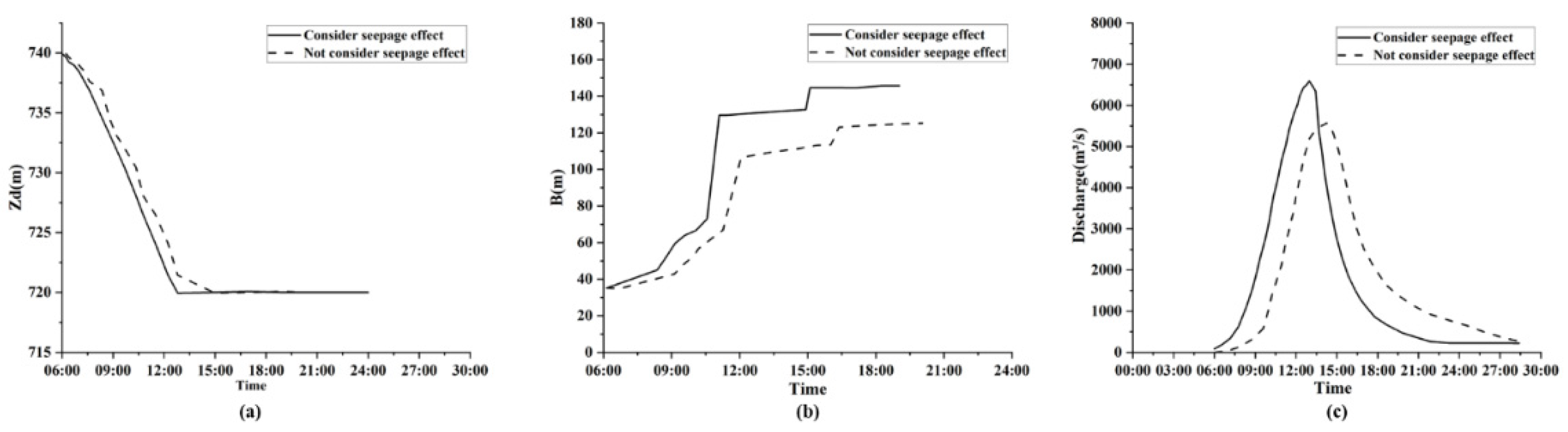
3.2.2. Influence of the Infiltration Module

The sensitivity analysis of the seepage module primarily focuses on evaluating the impact of the seepage effect while disregarding its influence. As shown in Figure 15, the seepage effect has a minimal impact on the bottom elevation of the breach, but it has a substantial impact on the breach width and outflow discharge. The seepage module has an impact on various aspects of the dam breach. It results in a wider ultimate breach width, a faster breach development rate, an increase in the breach peaking discharge, an earlier occurrence of the breach peaking discharge, and a shorter duration of the dam break. The seepage effect reduces the critical beginning velocity of the dam particles, increases the lateral extension rate of the breach, and makes it easier to fulfill the critical collapse condition.

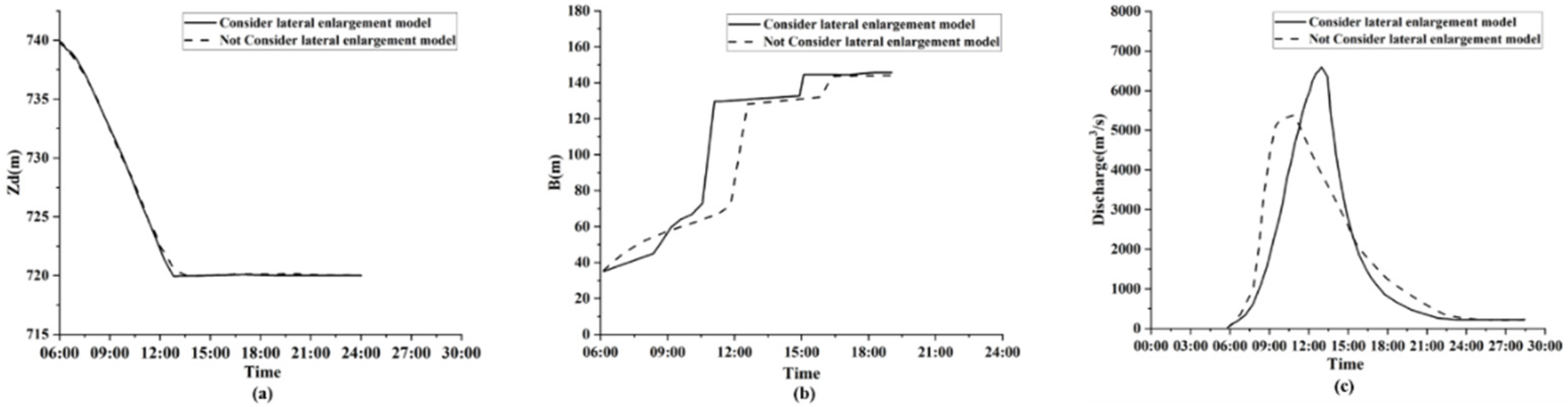
3.2.3. Influence of the Breach Lateral Evolution Module

This study primarily conducts a sensitivity analysis of the lateral evolution module by comparing and assessing the impact of the double linear expansion module and the enlargement module on the peaking discharge Q, breach bottom elevation Zd, and breach breadth B. As shown in Figure 16a,b, the lateral evolution module has minimal impact on the bottom elevation Z and the final width B of the breach, but significantly affects the rate at which the width B of the breach expands. The lateral evolution model accelerates the rate at which the breach breadth develops. Figure 16c demonstrates that it significantly affects the discharge mechanism of the breach, resulting in a higher peak discharge and a delayed arrival time.

4. Conclusions

This study developed an improved model to replicate the complete sequence of events, encompassing the hydrodynamic phenomena in the reservoir area, the progression of dam breach, and the spread of flooding in the downstream inundation area. The model comprises four modules: breach initiation assessment with or without infiltration, vertical erosion of the breach, lateral development of the breach, and slope stability. Furthermore, it is seamlessly incorporated with a two-dimensional flood model that is based on open-source technology and makes use of several central processing units (CPUs) and graphics processing units (GPUs).

Our salient contribution can be summarized as: (1) In the evolution model of the breach, the critical starting velocity formulas with and without seepage influence are established. (2) Based on the theoretical analysis of the initial movement of slope sediment, the lateral evolution formula for calculating the width of the breach is derived. (3) The iteration of each time step is realized by directly updating the DEM of the computational grid, and no special processing of the computational grid flux is needed. (4) The upstream reservoir area is included in the whole computational domain to participate in the calculation, and the water depth of the reservoir area in each time step reflects the change in the water volume in the reservoir area, which can simulate the two-dimensional hydrodynamic process of the reservoir area. At the same time, the water depth and flow velocity of the previous time step are used as the driving force for the evolution of the outburst in the next time step, avoiding the calculation process of the outburst flow by using the weir formula.

The reliability, adaptability, and efficiency of the integrated coupling model are confirmed through comparison analysis and sensitivity analysis, using the Taum Sauk dam and Tangjiashan Barrier Lake as application cases. The obtained results demonstrate strong concurrence with the measured data. In the Taum Sauk dam, the relative errors of the four important parameters, the peak discharge of the breach, the top width of the final breach, the depth of the breach, and the arrival time of the maximum peak discharge are all within ±10%. Although the relative error of the completion time of the final breach is greater than 10%, it is about 30% less than the relative error of the physical model.

However, the model presented in this paper has three limitations. Firstly, it does not take into account the erosion process of the downstream slope during the breach evolution. Secondly, the model is only capable of simulating a single breach in the dam and cannot simulate multiple breaches. Thirdly, the model cannot simulate piping failure. In the future, we will carry out physical tests to verify the model parameters. We will enhance the physical process of the breach evolution model and expand its range of applicability. Simultaneously, the further examination of various breaches and the superimposition of breaches in the dam should be conducted to verify that the simulation scenarios and outcomes closely resemble reality.

References

1. Li, W.; Li, Z.; Ge, W.; Wu, S. Risk Evaluation Model of Life Loss Caused by Dam-Break Flood and Its Application. Water 2019, 11, 1359. [Google Scholar] [CrossRef]
2. World Meteorological Organization Report. Provisional State of the Global Climate 2023; United Nations Publications: New York, NY, USA, 2023. [Google Scholar]
3. Mirauda, D.; Albano, R.; Sole, A.; Adamowski, J. Smoothed Particle Hydrodynamics Modeling with Advanced Boundary Conditions for Two-Dimensional Dam-Break Floods. Water 2020, 12, 1142. [Google Scholar] [CrossRef]
4. ICOLD. Lessons from Dam Incidents; ICOLD: Paris, France, 1975. [Google Scholar]
5. Zhong, Q.; Wu, W.; Chen, S.; Wang, M. Comparison of simplified physically based dam breach models. Nat. Hazards 2016, 84, 1385–1418. [Google Scholar] [CrossRef]
6. Esin, A. Prediction of the cyclic hardening stress—strain curve. J. Strain Anal. Eng. Des. 1980, 15, 235–237. [Google Scholar] [CrossRef]
7. Cecilio, C.B.; Tsay, K.D. Discussion of ‘Breaching Characteristics of Dam Failures’ by Thomas C. MacDonald and Jennifer Langridge-Monopolis (May, 1984). J. Hydraul. Eng. 1985, 111, 1123–1125. [Google Scholar] [CrossRef]
8. U.S. Bureau of Reclamation (USBR). Downstream Hazards Classification Guidelines; U.S. Bureau of Reclamation: Denver, CO, USA, 1995.
9. Vonthun, J.; Gillette, D. Guidance on Breach Parameters; U.S. Bureau of Reclamation: Denver, CO, USA, 1990.
10. Froehlich, D.C. Peak Outflow from Breached Embankment Dam. J. Water Resour. Plan. Manag. 1995, 121, 90–97. [Google Scholar] [CrossRef]
11. Froehlich, D.C. Predicting Peak Discharge from Gradually Breached Embankment Dam. J. Hydrol. Eng. 2016, 21, 04016041. [Google Scholar] [CrossRef]
12. Xu, Y.; Zhang, L.M. Breaching Parameters for Earth and Rockfill Dams. J. Geotech. Geoenvironmental Eng. 2009, 135, 1957–1970. [Google Scholar] [CrossRef]
13. Mei, S.; Chen, S.; Zhong, Q. Parametric model for breaching analysis of earth-rock dam. Adv. Eng. Sci. 2018, 50, 7. [Google Scholar]
14. Singh, V.P.; Scarlatos, C.A. Breach erosion of earthfill dams and floodrouting: BEED model. Nat. Hazards 1985, 1, 161–180. [Google Scholar] [CrossRef]
15. Fread, D.L. BREACH: An Erosion Model for Earthen Dam Failure; Hydrologic Research Laboratory, National Weather Service, NOAA: Silver Spring, MD, USA, 1988.
16. Mohamed, A.A.A.; Samuels, P.G.; Morris, M.W.; Ghataora, G.S. Improving the accuracy of prediction of breach formation through embankment dams and flood embankments. In Proceedings of the Conference on Fluvial Hydraulics (River Flow 2002), Louvain-la-Neuve, Belgium, 4–6 September 2002. [Google Scholar]
17. Morris, M.; Hassan, M.; Kortenhaus, A.; Geisenhainer, P.; Visser, P.; Zhu, Y. Modelling breach initiation and growth. In Flood Risk Management: Research and Practice: CRC Press: Boca Raton, FL, USA, 2008; pp. 581–591. [CrossRef]
18. Temple, D.M.; Hanson, G.J.; Neilsen, M.L. WINDAM—Analysis of Overtopped Earth Embankment Dams. In Proceedings of the 2006 ASAE Annual Meeting, Portland, Oregon, 9–12 July 2006. [Google Scholar]
19. Wu, W. Simplified Physically Based Model of Earthen Embankment Breaching. J. Hydraul. Eng. 2013, 139, 837–851. [Google Scholar] [CrossRef]
20. Zhong, Q.; Chen, S.; Deng, Z. Breach mechanism and numerical modeling of barrier dam due to overtopping failure. Sci. Sin. Technol. 2018, 48, 959–968. [Google Scholar] [CrossRef]
21. Graf, W.H. Hydraulics of Sediment Transport; Water Resources Publications: Littleton, CO, USA, 1971. [Google Scholar] [CrossRef]
22. Chen, Z.; Ma, L.; Yu, S.; Chen, S.; Zhou, X.; Sun, P.; Li, X. Back Analysis of the Draining Process of the Tangjiashan Barrier Lake. J. Hydraul. Eng. 2015, 141, 05014011.1–05014011.14. [Google Scholar] [CrossRef]
23. Wang, Z.; Bowles, D.S. Three-dimensional non-cohesive earthen dam breach model. Part 1: Theory and methodology. Adv. Water Resour. 2006, 29, 1528–1545. [Google Scholar] [CrossRef]
24. Cao, Z.; Yue, Z.; Pender, G. Landslide dam failure and flood hydraulics. Part II: Coupled mathematical modelling. Nat. Hazards 2011, 59, 1021–1045. [Google Scholar] [CrossRef]
25. Liu, W.; He, S. Dynamic simulation of a mountain disaster chain: Landslides, barrier lakes, and outburst floods. Nat. Hazards 2018, 90, 757–775. [Google Scholar] [CrossRef]
26. Zhang, D.; Li, D.; Chen, Z. Coupled one-and two-dimensional hydrodynamic models for levee-breach flood and its application. J. Hydroelectr. Eng. 2010, 29, 149–154. [Google Scholar]
27. Xiong, Y. A Dam Break Analysis Using HEC-RAS. J. Water Resour. Prot. 2011, 3, 370–379. [Google Scholar] [CrossRef]
28. DHI Water Environment. A Modelling System for Rivers and Channels User Guide; DHI Water Environment: Cambridge, CA, USA, 2012. [Google Scholar]
29. Zhang, D.; Quan, J.; He, X.; Dong, T. Development and application of 1D dam-break flood analysis system based on GIS. J. Hydraul. Eng. 2013, 44, 1475–1481. [Google Scholar]
30. Annunziato, A.; Dogan, G.G.; Yalciner, A.C. Modeling Dam Break Events Using Shallow Water Model. Eng 2023, 4, 1851–1870. [Google Scholar] [CrossRef]
31. Liu, J.; Li, Z.; Mei, C.; Wang, K.; Zhou, G. Urban flood analysis for different design storm hyetographs in Xiamen Island based on TELEMAC-2D. Chin. Sci. Bull. 2019, 64, 2055–2066. [Google Scholar] [CrossRef]
32. Albu, L.-M.; Enea, A.; Iosub, M.; Breabăn, I.-G. Dam Breach Size Comparison for Flood Simulations. A HEC-RAS Based, GIS Approach for Drăcșani Lake, Sitna River, Romania. Water 2020, 12, 1090. [Google Scholar] [CrossRef]
33. Hu, X.; Zhang, X. Application of mathematical model for dam-break flood flow. Eng. J. Wuhan Univ. 2011, 44, 178–181. [Google Scholar]
34. Ma, L.; Hou, J.; Zhang, D. Study on 2-D numerical simulation coupling with breach evolution in flood propagation. J. Hydraul. Eng. 2019, 50, 15. [Google Scholar]
35. Bladé, E.; Cea, L.; Corestein, G.; Escolano, E.; Puertas, J.; Vázquez-Cendón, E.; Dolz, J.; Coll, A. Iber: Herramienta de simulación numérica del flujo en ríos. In Revista Internacional de Métodos Numéricos para Cálculo y Diseño en Ingeniería; Elsevier: Amsterdam, The Netherlands, 2014; Volume 30, pp. 1–10. [Google Scholar]
36. MITECO. Technical Guide for the Classification of Dams; Ministerio Para la Transición Ecológica y el Reto Demográfico(MITECO): Madrid, Spain, 2021.
37. Xu, D.; David, P.; Ji, C.; Xu, B.; Liu, H. Simulation of Flood Propagation in Cities Using Large Scale Parallel Computation of Shallow Water Equations. J. Tianjin Univ. (Sci. Technol.) 2016, 4, 341–348. [Google Scholar]
38. Liang, Q.; Xia, X.; Hou, J. Catchment-scale High-resolution Flash Flood Simulation Using the GPU-based Technology. Procedia Eng. 2016, 154, 975–981. [Google Scholar] [CrossRef]
39. Morales-Hernández, M.; Sharif, B.; Kalyanapu, A.; Ghafoor, S.; Dullo, T.; Gangrade, S.; Kao, S.-C.; Norman, M.; Evans, K. TRITON: A Multi-GPU open source 2D hydrodynamic flood model. Environ. Model. Softw. 2021, 141, 105034. [Google Scholar] [CrossRef]
40. Echeverribar, I.; Morales-Hernández, M.; Brufau, P.; García-Navarro, P. 2D numerical simulation of unsteady flows for large scale floods prediction in real time. Adv. Water Resour. 2019, 134, 103444. [Google Scholar] [CrossRef]
41. Shao, X.; Wang, X. Introduction to River Mechanics, 2nd ed.; Tsinghua University Press: Beijing, China, 2013. [Google Scholar]
42. Han, Q.; He, M. The Threshold Motion of Sediment and Its Starting Speed; Science Press: Beijing, China, 1999. [Google Scholar]
43. Martin, C.S. Effect of a Porous Sand Bed on Incipient Sediment Motion. Water Resour. Res. 1970, 6, 1162–1174. [Google Scholar] [CrossRef]
44. Lauer, J.W.; Parker, G. Modeling framework for sediment deposition, storage, and evacuation in the floodplain of a meandering river: Application to the Clark Fork River, Montana. Water Resour. Res. 2008, 44. [Google Scholar] [CrossRef]
45. Wang, L.; Chen, Z.; Zhang, Q.; Chen, S.; Jin, S.; Zhong, Q. Back analysis of the breach flood of the “11.03” Baige barrier lake at the Upper Jinsha River. Sci. Sin. Technol. 2020, 50, 763–774. [Google Scholar] [CrossRef]
46. Chen, Z.; Ping, Z.; Wang, N.; Yu, S.; Chen, S. An approach to quick and easy evaluation of the dam breach flood. Sci. China Technol. Sci. 2019, 62, 1773–1782. [Google Scholar] [CrossRef]
47. Annandale, G.W. Scour Technology-Mechanics and Engineering Practice; Mcgraw-Hill: New York, NY, USA, 2006. [Google Scholar]
48. Zhong, Q.M.; Chen, S.S.; Mei, S.A.; Cao, W. Numerical simulation of landslide dam breaching due to overtopping. Landslides 2017, 15, 1183–1192. [Google Scholar] [CrossRef]
49. Zhong, Q.; Chen, S.; Shan, Y. Numerical modeling of breaching process of Baige dammed lake on Jinsha River. Adv. Eng. Sci. 2020, 52, 29–37. [Google Scholar]
50. Cai, Y.; Zhang, X.; Xue, R.; Wang, M.; Deng, Q. Numerical simulation of overtopping breach processes caused by failure of landslide dams. Environ. Fluid Mech. 2022, 22, 839–863. [Google Scholar] [CrossRef]
51. Singh, V.P. Dam Breach Modeling Technology; Springer Nature: Dordrecht, The Netherlands, 1996. [Google Scholar]
52. Froehlich, D.C. Embankment Dam Breach Parameters Revisited; American Society of Civil Engineers: Reston, VA, USA, 1995. [Google Scholar]
53. Fread, D.L. The NWS Dam Break Flood Forecasting Model; National Oceanic and Atmospheric Administration: Washington, DC, USA, 1984.
54. Mei, S.; Zhong, Q.; Yang, M.; Chen, S.; Shan, Y.; Zhang, L. Overtopping-Induced breaching process of concrete-faced rockfill dam: A case study of Upper Taum Sauk dam. Eng. Fail. Anal. 2023, 144, 106982. [Google Scholar] [CrossRef]
55. Kalyanapu, A.J.; Shankar, S.; Pardyjak, E.R.; Judi, D.R.; Burian, S.J. Assessment of GPU computational enhancement to a 2D flood model. Environ. Model. Softw. 2011, 26, 1009–1016. [Google Scholar] [CrossRef]
56. Rydlund, P.H. Peak Discharge, Flood Profile, Flood Inundation, and Debris Movement Accompanying the Failure of the Upper Reservoir at the Taum Sauk Pump Storage Facility near Lesterville, Missouri, U.S, Geological Survey Scientific Investigations Report; U.S. Geological Survey: Reston, VA, USA, 2010.
57. Zhong, Q.; Chen, S.; Zhao, L.; Ren, Q.; Cao, W. Numerical simulation of overtopping failure process of a barrier dam. Joumal Hohai Univ. (Nat. Sci.) 2012, 40, 7. [Google Scholar]
58. Hu, X.; Luo, G.; Wang, J. Seepage stability analysis and dam-breaking mode of Tangjiashan barrier dam. Chin. J. Rock Mech. Eng. 2010, 29, 1409–1417. [Google Scholar]
59. Zhong, Q.M.; Chen, S.S.; Deng, Z. Numerical model for homogeneous cohesive dam breaching due to overtopping failure. J. Mt. Sci. 2017, 14, 571–580. [Google Scholar] [CrossRef]
Figure 1. Force analysis of soil particles.
Applsci 14 10921 g001
Figure 2. Diagram of forces acting on a particle in the slope.
Applsci 14 10921 g002
Figure 3. Schematic diagram of the collapse and expansion process of the dam breach.
Applsci 14 10921 g003
Figure 4. The schematic diagram of the integrated model.
Applsci 14 10921 g004
Figure 5. The flow chart of the model.
Applsci 14 10921 g005
Figure 6. The Taum Sauk dam location and the shape of the breach: (a) breach frontal view; (b) breach top view; (c) dam location; (d) study area remote sensing image.
Applsci 14 10921 g006
Figure 7. The diagram of the dam profile and initial breach: (a) side view; (b) top view.
Applsci 14 10921 g007
Figure 8. Study area and topographic of Tangjiashan barrier dam.
Applsci 14 10921 g008
Figure 9. The results of the breach flow process for different models of Taum Sauk.
Applsci 14 10921 g009
Figure 10. Diagram of the development of the breach in Taum Sauk.
Applsci 14 10921 g010
Figure 11. The Comparison between the measured and the simulated of the Tangjiashan landslide dam failure: (a) outflow discharge; (b) breach width; and (c) breach bottom elevation.
Applsci 14 10921 g011
Figure 12. Water depth maps of the upstream and downstream at different times of Tangjiashan dam break flood.
Applsci 14 10921 g012
Figure 13. Simulated and measured discharge results of typical section Beichuan and Tongkou.
Applsci 14 10921 g013
Figure 14. Comparison of the simulated results with different erodibility parameters for Tangjiashan barrier dam: (a) breach bottom elevation; (b) breach width; and (c) outflow discharge.
Applsci 14 10921 g014
Figure 15. Comparison of sensitivity analysis results of seepage module of Tangjiashan barrier dam: (a) breach bottom elevation; (b) breach width; and (c) outflow discharge.
Applsci 14 10921 g015
Figure 16. Comparison of sensitivity analysis results of lateral evolution module of Tangjiashan barrier dam: (a) breach bottom elevation; (b) breach width; and (c) outflow discharge.
Applsci 14 10921 g016