Establishing Lightweight and Robust Prediction Models for Solar Power Forecasting Using Numerical–Categorical Radial Basis Function Deep Neural Networks

Abstract

As green energy technology develops, so too grows research interest in topics such as solar power forecasting. The output of solar power generation is uncontrollable, which makes accurate prediction of output an important task in the management of power grids. Despite a plethora of theoretical models, most frameworks encounter problems in practice because they assume that received data is error-free, which is unlikely, as this type of data is gathered by outdoor sensors. We thus designed a robust solar power forecasting model and methodology based on the concept of ensembling, with three key design elements. First, as models established using the ensembling concept typically have high computational costs, we pruned the deep learning model architecture to reduce the size of the model. Second, the mediation model often used for pruning is not suitable for solar power forecasting problems, so we designed a numerical–categorical radial basis function deep neural network (NC-RBF-DNN) to replace the mediation model. Third, existing pruning methods can only establish one model at a time, but the ensembling concept involves the establishment of multiple sub-models simultaneously. We therefore designed a factor combination search algorithm, which can identify the most suitable factor combinations for the sub-models of ensemble models using very few experiments, thereby ensuring that we can establish the target ensemble model with the smallest architecture and minimal error. Experiments using a dataset from real-world solar power plants verified that the proposed method could be used to build an ensemble model of the target within ten attempts. Furthermore, despite considerable error in the model inputs (two inputs contained 10% error), the predicted NRMSE of our model is still over 10 times better than the recent model.

1. Introduction

Worldwide, solar power is being incorporated into power grids to replace highly polluting power generation methods such as burning fossil fuels. While this is sure to reduce damage to the earth’s environment and aid in our quest for sustainable development, solar power is inherently uncontrollable and intermittent. It relies on hours of sunlight, the intensity of which is subject to natural phenomena such as cloud cover and rainfall. Thus, incorporating solar power into the power grids of large regions can cause unstable grid frequencies, severe power surges, and even power grid failures. To overcome this issue, power grid management teams mostly use solar power forecasting technologies based on weather forecasting data to predict the power output at the next time point. The output provided by solar power is then stabilized using other types of power such as thermal power or hydropower plants [1,2]. This means solar power forecasting is a key technology for countries developing green energy, and as such, it has been widely studied.

Researchers have utilized physical, statistical, and machine learning models to study solar power forecasting. Physical models consider weather variables such as illuminance, relative humidity, wind speed, and wind direction [3,4,5]. Over the long term, this approach proves accurate when weather conditions are stable, but prediction accuracy declines greatly when weather factors fluctuate. Many researchers therefore suggested replacing physical models with statistical methods because the latter can identify patterns in large amounts of historical data and provide accurate prediction results even when weather conditions vary [6,7,8]. In recent years, however, researchers pointed out that for most nonlinear prediction problems such as solar power forecasting, machine learning methods can offer more accurate results. Subsequently, machine learning methods became the mainstream in solar power forecasting research; for instance, decision trees [9,10], random forests [11,12], and neural networks [13,14,15] were all demonstrated to be effective on the target problem. The most popular models were deep learning models [16,17,18], because compared to other machine learning methods, their massive network architectures can better learn the subtleties of the nonlinear factors in the target problem to provide outstanding prediction results. On the whole, the advent of deep learning models has enabled solar power forecasting to become highly accurate. Thus, the focus has shifted from increasing accuracy to overcoming difficulties encountered in practice.

In studies using machine learning models to predict solar power generation, various sensors such as light meters, rain gauges, and hygrometers are first set up around the solar power plant, and then, various models are established to investigate the relationship between sensor data and power output. However, in real-world environments, the prediction values of this approach can be inaccurate due to problems with the sensors. Sensors consist of electronic components; thus, in addition to the aging of the components themselves causing measurements to gradually lose accuracy, their operation in extreme environments with high sun exposure, high temperatures, heavy rainfall, or humid air can easily damage components and affect the accuracy of their measurement results. For the solar power plants discussed in this study, it is necessary to install sensors outdoors to collect environmental data, so sensor wear is likely to be more severe than that in other applications, increasing the possibility of inaccuracy. Furthermore, sensor wear occurs irregularly, and power plants do not have enough personnel to closely monitor and replace sensors. Therefore, ensuring that machine learning models can output accurate prediction results despite inaccurate sensor values has become a crucial issue.

In the field of machine learning, the requirement for models to produce accurate values while receiving inaccurate input is referred to as a ‘robust prediction’ problem [19,20,21]. This concept has been applied to a number of fields such as automatic control [22,23,24] and traffic flow prediction [25,26,27]. In solar power generation, research on this topic can be roughly divided into three categories. The first category preprocesses and calibrates the inputs before model calculations to avoid values with excessive errors in the inputs. This prevents model calculations from producing results with excessive errors [28,29,30]. However, this approach requires identification of the errors before modeling, so that the model developers know how to preprocess and calibrate the values. Clearly, this is not suitable for the abnormalities that occur in sensors because we cannot know when and what types of errors will occur. This will also, of course, make it difficult to design a suitable processing method. The methods in the second category use broad standards to shield the impact of these errors on the model calculation results without knowing the type of error that has occurred [29,31]. A variety of ways exist to implement such methods. For instance, researchers [31] set the upper and lower bounds of model loss functions as constants to suppress the impact of abnormal values on output results. Other researchers [29,32] added random noise to training datasets so that the model would know how to process various types of noise from the outset. Nevertheless, we must understand that such methods require a broad standard to be set beforehand to serve as the basis of implementation. However, the input factors that solar power forecasting considers are all weather data, which by nature are extremely diverse and significantly influence one another. Thus, it would be difficult for us to find a broad standard to implement this concept. Finally, the methods in the third category avoid the influence of input errors on model outputs via ensemble modeling [1,2,33,34,35]. These methods claim that the information received by different models may vary but can all produce similar model output results. Even if some of the model inputs contain errors affecting some of the model outputs, the ensemble of models can weaken the effects of these output errors through the unaffected models, thereby achieving robustness. On the whole, this approach does not require investigating the possible types and range of errors. We therefore selected this as the primary approach for this paper. The greatest shortcoming of the third category of methods is that it increases the amount of model computations enormously, particularly when the existing models were all developed based on deep learning. We therefore propose a novel approach which involves pruning the deep learning model architecture to reduce the amount of computation in each sub-model in ensemble learning and thereby reduce the amount of computation in the overall ensemble learning model.

In the past, reducing the computation associated with deep learning models was mostly achieved by pruning the model architecture, which involves first training a deep learning model and then analyzing the model parameters and removing the parameters with the least contribution to model outputs. The three techniques most commonly applied for pruning are shown in Figure 1. In order of development, they are (1) pruning model weights, (2) pruning entire hidden layers, and (3) pruning unnecessary input factors. Researchers who employed the first technique [36,37,38,39] believed that if the weight between two layers of neurons in a model is close to 0, then no matter what the output of the previous layer of neuron is, the value is returned to 0 by the weight once it is passed on to the later layer of neurons. In other words, the outputs of the previous layer of neurons have no impact on the final outputs of the model. Thus, parameters with near-zero weights are pruned. This approach has been shown to effectively reduce the amount of computation via experimental simulations. However, some researchers [40,41,42] have discovered that such methods were not helpful in practice because pruning some of the weights in a deep learning model causes their weight matrices to become sparse. Many existing deep learning models are computed using GPUs in the real world; at present, GPUs will fill in missing values with 0 when calculating sparse matrices and then treat them as complete matrices, which means that the amount of computation has not been reduced. A number of researchers [42,43] therefore proposed pruning entire hidden layers would be more effective than simply pruning several weights. The sum of the weights in each hidden layer is calculated, and hidden layers with a weight sum below a certain threshold are regarded as excessive and thus are removed. Clearly, this approach can prevent GPUs from performing unnecessary calculations, ultimately reducing computation. However, it has been said that this approach merely treats the symptoms but does not cure the disease. Early on in the development of deep learning theory, many stressed that all of the factors that could be collected into the network should be included before using the massive network architecture to clarify the relationships between each factor and the model outputs. However, while conducting explainability analysis of models in recent years, many researchers found that many input factors of deep learning models are actually of no help to the output, and including these useless input factors comes at great cost to architecture size and computation. For this reason, Refs. [44,45,46,47,48] proposed the framework shown in Figure 2 to establish models with high precision but reduced computation costs. In this framework, researchers similarly define, establish, and train a suitable deep learning model, extract the key features identified by the trained model, and construct a model using only these key features and lightweight model. The lightweight models established using this framework have much fewer input factors and highly reduced computation, but their accuracy is not that much lower than that of the original deep learning model. This was the approach selected for the current paper.

We designed a novel methodology based on the concept depicted in Figure 2 to perform robust predictions for solar power generation at extremely low cost. Figure 3 displays the operating framework of our novel methodology. In the first phase, we similarly establish and train a deep learning model. Next, we analyze the parameters of the trained model to rank the factors according to their importance to solar power forecasting. In the second phase of the methodology, we identify multiple factor combinations with the least number of testing in the importance ranking from the first phase. Next, we establish lightweight models for each of the factor combinations so that they can all generate near-optimal prediction results. Finally, we perform ensemble calculations of the outputs of the lightweight models. These results are robust, as the lightweight models each use different factor combinations, so when errors occur in some of the factors, they will only affect a small number of the lightweight models and not all of them. Furthermore, once we perform ensemble calculations of the lightweight model outputs, the errors in some of the factors in the small number of lightweight models will be further weakened, thereby achieving robustness.

In the first phase of our methodology, we designed a model based on the radial basis function deep neural network (RBF-DNN) [49,50,51,52], which consists of a common deep neural network (DNN) with a radial basis function (RBF) layer added in the front. We chose this model for two reasons. First, the input factors discussed in the problem of this paper are weather factors, and the greatest difficulty in processing such datasets is that the distributions of the factor data are extreme; in addition to the normally-distributed factors (Figure 4a), there are also factors whose data are concentrated at the minimum value end of the x axis (Figure 4b) or at both the minimum and maximum value ends of the x axis (Figure 4c). Past studies [52,53,54] have demonstrated that adding an RBF layer in front of the model is an effective way of modeling such data. This is because RBFs have classifier characteristics, which enable the model to classify the values of each group of input data before deriving the relationships between the inputs and the outputs based on the classification results. Second, unlike the method of using the outputs of the hidden layers in deep learning models to obtain key features, the input factors of RBF deep learning models can be directly regarded as key features, which is more convenient for online applications. To use the outputs of a specific hidden layer as the key features, online applications require all the calculations of the original deep learning model from the input layer to said hidden layer, as shown in Figure 5. Directly using the model inputs as the key features of the lightweight models avoids these calculations.

Although the concept of RBF-DNNs is well-suited to the topic of this study, the details of the model must be adjusted for the target problem, due to two underlying issues. First, RBF-DNNs designed in the past only considered numerical factors and are not suitable for categorical factors. However, categorical factors such as the model of the solar panel or the subarea of a power plant are common in solar power forecasting. We therefore modified existing RBF-DNN architecture so that it can process categorical factors as well as numerical factors. This modification is depicted by the gray box of Phase 1 in Figure 3. To differentiate it from conventional RBF-DNNs, we refer to the modified model as a numerical–categorical RBF-DNN (NC-RBF-DNN). Second, conventional RBF-DNNs mostly obtain key factors by setting threshold values to extract the top several key factors and then constructing the subsequent lightweight models. In other words, these methods can only identify the input factors that are the most important for modeling; the importance of the other factors is unknown. In the current paper, we propose using the ensembling concept to establish sub-models for multiple input factor combinations to obtain the importance ranking of all of the factors.

In the second phase of our methodology, we designed a heap-based factor combination search algorithm to generate combinations of the inputs of the multiple sub-models based on the factor importance ranking obtained by the NC-RBF-DNN. This design was devised separately because the key factors that an RBF-DNN extracts vary with each iteration [52,53]. For instance, the importance ranking of the key factors extracted may be A, B, and C in the first training but C, A, and D in the next training. This is due to the powerful modeling capabilities of deep learning models. For example, let us assume there are two input factors to a model. Even if the two factors are only moderately correlated to each other from a relational perspective, the model may only choose one of the factors as the primary factor for modeling and regard the other as useless. This is because the model can use its massive model architecture to capture the complex relationships between the primary factor and the output without the information provided by the other input factor. Furthermore, the parameters of deep learning models vary during each initialization, so the key factors that are selected after each training will also differ, thereby affecting the factor importance ranking results produced by the model. In other words, using the importance ranking of these factors for modeling has its flaws, so we designed another selection method to obtain sub-models similar in precision using the smallest number of combination checks and achieve robust prediction via ensembling. Implementation with data from a real-world solar power plant verified the validity of the proposed methodology.

The current paper makes three important contributions to the topic of solar power forecasting:

• This is the first study to incorporate the concepts of ensemble models and lightweight deep learning models into robust predictions of solar power generation.
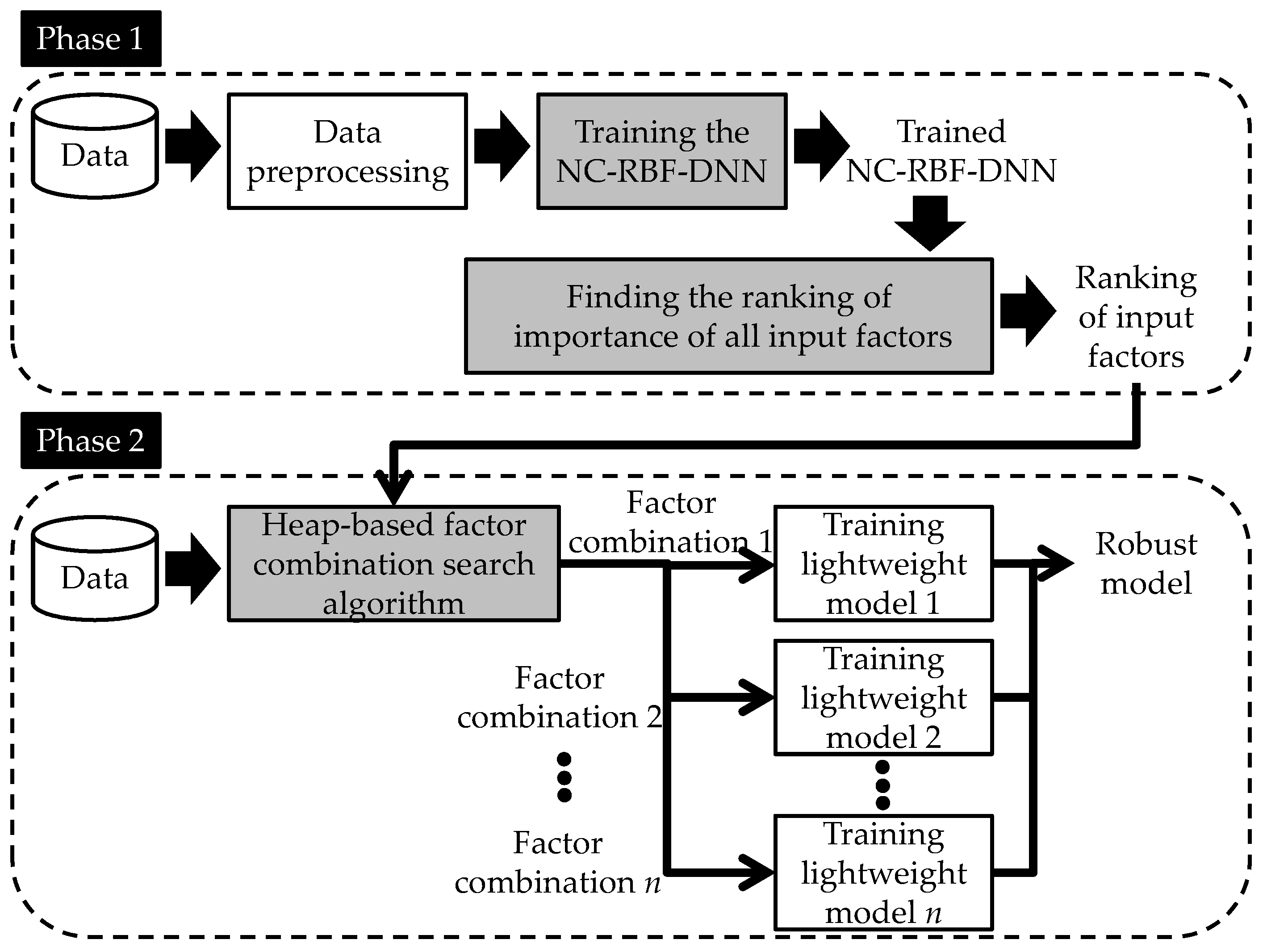
• We customized an NC-RBF-DNN based on the distribution characteristics of the input factor data of solar power forecasting to establish lightweight models using the train–dismantle deep learning model method.
• We designed a heap-based factor combination search algorithm to find multiple combinations of suitable factors based on the factor importance ranking obtained by the NC-RBF-DNN; after the factor combinations are input to the lightweight models, they produce near-optimal prediction results.

The remainder of this paper is arranged as follows. Section 2 reviews related works, Section 3 presents our methods, Section 4 explains our experimental simulations, and Section 5 contains the conclusions.

2. Related Works

2.1. Related Works: Solar Power Forecasting

This section introduces existing solar power forecasting models in their three categories: physical, statistical, and machine learning models. We also introduce how researchers extended existing models to enhance their robustness.

First are the physical models, the concept of which is to first identify the factors that affect solar power generation and then use these factors for modeling. Two major branches of factors were considered: weather factors [3,4,5] and circuit board factors [55,56,57]. With regard to weather factors, Salinas et al. [3] developed a physical model for the central region of Chile to predict the solar refractive index and power output in an area, based on area elevation and the day’s weather and cloud cover. The physical model established by Diagne et al. [4] indicated that the thickness and changes in cloud cover exert a direct impact on solar refraction and solar power generation. As for circuit board factors, Chaibi et al. [55] developed a physical model based on the photovoltaics and thermal collectors of solar power generation; their model could effectively predict the current solar thermal energy collected and the power efficiency brought by conversion. For the reliability, safety, and stability of power stations, Dolara et al. [56] designed a physical model for three types of photovoltaic cells with different circuit board parameters to estimate electromagnetic temperature and thermal resistance. These studies all claimed that their models were effective. However, most researchers now believe that the process of searching for factors for physical models is time-consuming and prone to errors, so physical models have gradually fallen out of favor in recent years.

With regard to statistical models, researchers have attempted to achieve prediction objectives using linear and nonlinear models [58,59]. In linear models, Sopian and Othman [60] used the least squares method and a linear regression algorithm to analyze the relationship between the average daily solar radiation and sunshine hours for each month, based on data collected from eight different cities in Malaysia. Chineke et al. [61] similarly used linear regression to develop an Angström model to predict global solar radiation. The Angström model was later utilized by Khatib et al. [62] to calculate correlation coefficients and develop a solar power model. In nonlinear models, Boilley et al. [6] employed statistical principles to develop a prediction model using time series data to forecast photovoltaic output power. Using the autoregressive integrated moving average (ARIMA) algorithm, Dambrevill et al. [7] developed a statistical model for energy management in solar panels. Based on the direction and scale of architecture, Karteris et al. [8] created a mathematical regression model to predict solar power use.

Next, the popularity of machine learning models has risen because the technology has been demonstrated to be applicable to linear and nonlinear modeling for solar power forecasting [63]. Rahul et al. [9] employed a decision tree algorithm to predict the influence of different types of weather on solar power generation. Kassim et al. [10] used a decision tree algorithm to forecast the output power of a large-scale solar power plant. Mansoury et al. [64] developed a power generator with three energy sources—that is, solar power, battery, and diesel fuel—and used a decision tree to manage the three energy sources. Khalyasmaa et al. [11] utilized a random forest algorithm to reasonably distribute power supplied by a solar power plant while taking safety and reliability into consideration. Liu et al. [12] used the characteristics of random forest factor extraction to identify the crucial factors in solar power datasets and then performed modeling using only these crucial factors. Aside from the conventional machine learning models, many researchers have been exploring the efficacy of artificial neural networks. For instance, Mellt et al. [65] and Reddy and Ranjian [13] predicted solar radiation using an artificial neural network. Zarzalejo et al. [14] constructed a hybrid model combining neural networks and fuzzy logic to predict solar radiation in Spain based on satellite images and cloud cover data. Alam et al. [15] predicted solar radiation in certain areas using a multilayer perceptron, with latitude, longitude, elevation, month, sunshine ratio, rainfall, and humidity as inputs. Rajendran and Gebremedhin [66] established a model combining an EnergyPLAN system with neural networks. The EnergyPLAN system outputs the information of multiple power grids at the same time, and a trained neural network can effectively monitor several power grids.

Numerous researchers are advocating for the adoption of deep learning (DL) models as an alternative to machine learning models, with the aim of improving the accuracy of solar power generation predictions. Elsaraiti and Merabet [67] reported that long-short-term memory (LSTM) was superior to conventional multi-layer perceptron models in predicting solar power generation. Chang et al. [68] reported that their DL model, based on encoding, outperforms regression techniques. Sharadga et al. [69] added bidirectionality to LSTM to extend prediction results over longer durations. Some researchers have claimed that the relationship between weather factors and solar power generation is too complex for any single deep learning model, prompting the development of composite prediction models. AlKandari [70] integrated the Theta statistical method with LSTM and a Gated Recurrent Unit recurrent neural network (GRU) to improve prediction accuracy. Plessis et al. [71] integrated a feedforward deep learning model, LSTM, and GRU to capture the characteristics of solar power generation over various timeframes. Gensler et al. [16] developed a hybrid model based on a deep belief network, AutoEncoder, and LSTM to forecast the power output of solar power plants. Jamil et al. [18] merged multiple types of DL models to monitor and predict the power generation, soiling loss, and performance ratio of a large-scale power plant. Zhou et al. [17] created a hybrid model using LSTM and a convolutional NN (CNN) to forecast short-term variations in photovoltaic power output. Note that the methods mentioned above involve digitizing weather data and then inputting the numerical results into the model for prediction. By contrast, some scholars have recently begun exploring the possibility of predicting solar power generation by analyzing images of the sky. Pedro et al. [72] proposed the use of convolutional NNs to extract features from images for use in predicting solar power generation. Sun et al. [73] and Paletta et al. [74] respectively proposed the SUNSET model and ConvLSTM model, both of which have become benchmarks by which new methods are developed and tested. Nie et al. [75] developed a transfer learning framework based on the SUNSET model and ConvLSTM to reduce the amount of data required for model building. Some scholars have also tried combining images with other data. Maciel et al. [76] combined numerical weather data with data from sky images to improve the accuracy of their model.

Accuracy is not the only concern. As discussed, the sensors that collect data for prediction are subject to errors, introducing instability to solar power forecasting. Researchers have sought to overcome this issue in three ways. The first approach involves preprocessing the data to ensure that incorrect data are not input to the model. For instance, Zhang et al. [28], Sharma et al. [29], Peng et al. [30], and Colak and Qahwaji [77] all used wavelet models to first denoise the original solar radiation time series before inputting the denoised data into various models for power generation forecasting. These studies all verified the validity of their methods using historical data from real-world power plants. The second category of methods is based on a set of broad standards to shield the model computation results from the errors in the inputs. For instance, Zhang et al. [28] prevented abnormal input values from creating numerous errors in the output results by limiting the upper bound of the prediction model’s loss function to a constant, thereby ultimately achieving robustness. Monjoly et al. [78] recommended that models should be trained to output reasonable prediction values when the input contains errors so as to prevent them from outputting inappropriate results when online; the results of their simulation experiments served as proof of concept. Finally, the last category of methods ensembles multiple models with different inputs but the same prediction target. For instance, Liu and Sun [79] combined principal components analysis, k-mean, and random forest algorithms to create a hybrid model and applied it to solve instabilities in solar power generation. Subramania et al. [80] proposed a hybrid model with high precision in solar power forecasting. The model included support vector machines, decision trees, random forest, and gradient boosting to predict various factors, and they used precision, recall, and F1-score to verify the accuracy of the hybrid model predictions. Thorey et al. [33] first employed different methods to obtain various prediction results, used a technique called the continuous ranked probability score to give the prediction results different weights, and then ensembled the prediction results based on the weights. Bracale et al. [2] used different probability distributions to establish multiple models, competed these models against one another, and then used the three most accurate models for ensemble predictions. Raj et al. [19] recently established integrated models for existing machine learning models, such as gradient boosting machines, random forest, k-nearest neighbor, and support vector machines. Their results confirmed that this approach is highly intuitive and effective in dealing with multiple types of inputs, achieving extremely low prediction error even in the presence of input error. Researchers have also determined that clustering data prior to modeling helps in managing input error more effectively. Zhang et al. [34] ensembled different forecasting results using clustering and blending and then performed experiments to demonstrate that this approach could provide more robust forecasting results. Adopting the approach used by [34], Pan and Tan [35] conducted the cluster analysis of solar power generation to obtain weather conditions, established random forests with different parameters depending on different weather conditions, and then performed weighted calculations of the different random forest models to obtain the final results. More recently, Lotfi et al. [1] believed that conventional clustering methods may not be effective, so they performed clustering using kernel density estimation. In the online application, they first identified the cluster closest to the current conditions and then ensembled the model of said cluster for forecasting. They demonstrated through experiments that their approach was superior among clustering methods.

2.2. Related Works: Lightweight Deep Learning Models

Roughly five years ago, researchers began developing lightweight deep learning (DL) models to reduce computational overhead without adversely affecting the output. Lightweight methods can be divided into two categories: (1) those that delete useless weights or hidden layers and (2) those that delete input fields.

The first method developed for the deletion of unnecessary weights involved the use of second-order derivative information [36] or L1/L2-norm regularizations [39] to calculate the importance of each weight value to the overall output. Weight values that were shown to have little impact on the output were simply omitted. Nonetheless, scholars soon discovered that this approach transformed the model weights into a sparse matrix with numerous null values. In practice, the GPU fills in null values with zeros prior to commencing operations, thereby rendering this deletion method ineffective [40,41,42].

This prompted efforts to delete entire layers. Li et al. [40] used L1/L2-norm regularization to calculate the absolute weight sum of the filter layer in a DL model, assuming that the sum of weights could represent the degree of layer activation. Layers with greater activation can be expected to have a more pronounced impact on the output, indicating that they contain information of importance to that layer, which should be preserved. The layers with limited activation [40] are deleted to reduce the cost of constructing the DL model. Luo et al. [41] combined the greedy algorithm with a loss function to identify filter layers that contain information of importance to modeling. Molchanov et al. [42] used Taylor expansion to estimate the impact of the filter layer in the DL model on the loss function and, in so doing, determine whether the content should be preserved for modeling. Roy et al. [81] discovered that retraining was required after modifying the architecture of a DL model. This prompted their development of a program that allows simultaneous pruning and training to expedite the establishment of a DL with minimal cost. Wu et al. [82] proposed a framework to facilitate the pruning of the YOLO v4 architecture. The efficacy of their method was demonstrated in the detection of apple blossoms, outperforming other models commonly used in image processing in terms of accuracy and computational efficiency.

Many scholars prefer deleting input fields instead of weights, due to its relative simplicity and intuitiveness. Sani et al. [45] established a low-cost action recognition in which the key factors contained in the output of the last DL pooling layer are used as inputs for k-nearest neighbor modeling. Mohammad et al. [46] developed mathematical formulas for the disassembly of DL parameters to obtain key factors. The low-cost AI model built using these key factors achieved action recognition accuracy on par with that of DL models (DLMs). Chen et al. [48] and Chiu et al. [83] focused on the numerical modeling of map grids. They first used the Grad-Cam suite to obtain CNN results for all input grids. Even when applied to a relatively low-cost AI model, these key grids were sufficient to achieve modeling accuracy close to that of the original convolutional NN. Liu et al. [47] developed a semi-supervised learning model to overcome the challenge of obtaining EEG data samples. They first trained a CNN based on existing EEG and then developed a set of algorithms to derive essential features from EEG data. In experiments, their system proved highly effective in extracting essential features for analysis from limited EEG data. Chen and Lee [52] and Chiu et al. [53] reported that their DL model based on the radial basis function (RBF) could quickly identify the key inputs, achieving accuracy on par with a DL model even when paired with a lower-cost AI model.

3. Methods

Figure 3 displays the process used in this study to design a robust solar power forecasting model, including offline data preprocessing, training and dismantling the NC-RBF-DNN to rank all of the input factors by importance, and using a factor combination search algorithm to establish the multiple sub-models needed for the ensemble model. We introduce these three phases below.

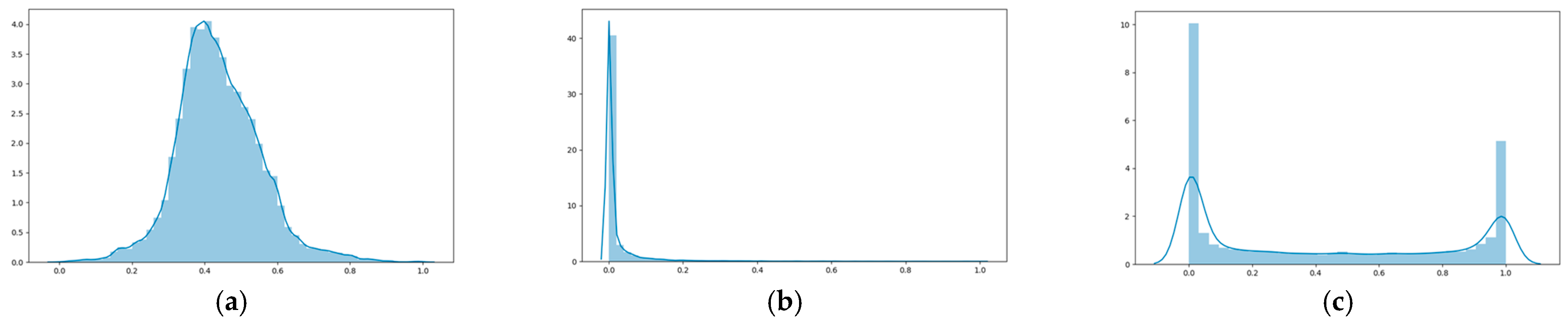
3.1. Preprocessing of Historical Weather Data

Weather data is usually collected by hardware equipment, so historical weather datasets are subject to data defects caused by hardware issues such as missing, null, or negative values. Including these values in modeling will reduce the accuracy of model predictions, so we employed linear interpolation to fill in missing values, as suggested in past studies [84,85]. If the range that needs filling in is shorter than 24 h, we use the values before and after the range for interpolation (as shown in Equation (1)). In this way, the filled-in values will best fit the conditions of the day. If the range that needs filling in is longer than 24 h, we use the means of the 24 h values before and after the range for interpolation (as shown in Equation (2)). In this way, the filled-in values will not be able to recreate the conditions of the day, but at least the data from the same periods of the day before and after can simulate likely weather conditions.

$$y(h+n)=y(h)+{\displaystyle \frac{n}{g+1}}(y(h+g+1)-y(h)),$$

(1)

$$y(t)={\displaystyle \frac{y(t+24)+y(t-24)}{2}}.$$

(2)

In the two equations above, y(•) represents the target time series, h denotes the time of the last normal item of data before the missing value range, g indicates the time length of the missing data, and n represents the prediction for the nth item of data that needs filling in, where g − 1 ≥ n ≥ 1.

3.2. Training and Dismantling NC-RBF-DNN to Obtain Importance Ranking of Factors

This section introduces the architecture of NC-RBF-DNN and the algorithm used to obtain the factor ranking.

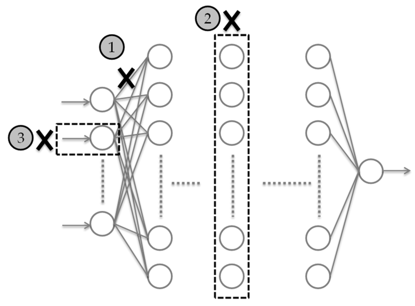
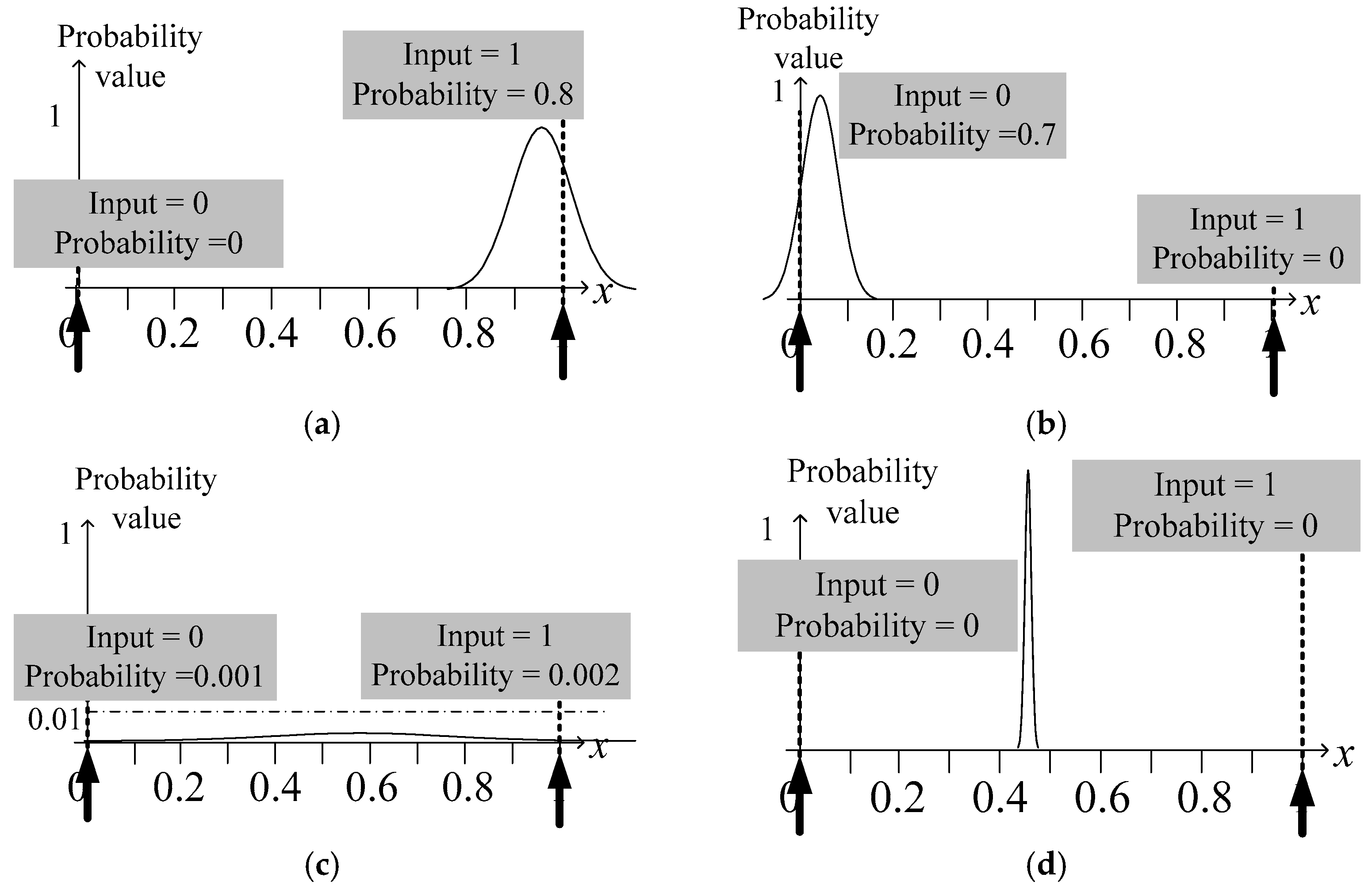
3.2.1. Architecture of NC-RBF-DNN

The NC-RBF-DNN architecture proposed in this study is similar to that of existing RBF-based deep learning models [53,54]; it similarly includes an input layer, an RBF layer, and a deep neural network (DNN) connected behind it, as shown in Figure 6. The input layer of the model is responsible for inputting the values of input factors into the model, whereas the RBF layer is responsible for classifying these input values and outputting the probability that each input value is placed in each class. These probabilities are then passed on to the following DNN to establish the relationship between these probabilities and the target outputs.

The greatest difference between the model design of NC-RBF-DNN and that of existing architectures is that it processes different types of input factors separately. As shown in Figure 6, the model is divided into two sub-networks for modeling in the input layer and RBF layer: one dedicated to processing numerical input factors and the other to processing categorical input factors. A lot of progress has already been made regarding the architecture for numerical input factors, and its performance has been verified [53,54]. We therefore adopted this architecture without any changes. That is, in the RBF layer, each input layer output has q neurons responsible for converting the inputs into q probabilities. Users can designate the value of q or use a Gaussian mixture model to determine the optimal value for q. Figure 7 illustrates this architecture [53,54]. If we suppose the output of an input layer has three neurons to convert it into probabilities, then the RBF conditions in either Figure 7a or Figure 7b indicate that the minimum and maximum output values of the input layer of the deep learning network differ, so the values of the input layer outputs obviously influence the final outputs of the model. In contrast, with the RBF conditions in Figure 7c,d, the function will output near-zero values no matter what the input layer outputs are, which means that the input layer outputs corresponding to the function will not influence the outputs of the subsequent deep learning model. Thus, the outputs of this input layer are not important.

The application of categorical input factors to this model is novel, so we designed the following approach. The input layer mainly performs one-hot encoding. If we suppose a factor has n categories of data, and the current input is of the mth category, we first convert the original category numbers into a vector [v₀, v₁, …, v_n], where v_m is 1 and the other values in the vector are all 0. Next, we input the values of this vector into respective neurons. In other words, the input factors of this categorical type are represented by n neurons in the input layer of the model. As for the RBF of this part, each input layer output will only have one neuron to convert it into a probability. Thus, each input layer output is either 0 or 1, meaning that we only need one RBF to convey the importance of an input layer output to the subsequent deep learning model. For instance, the RBF conditions in Figure 8a,b indicate that the 0 and 1 output values of the input layer of the deep learning network differ and have an influence on the model output. In contrast, with the RBF conditions in Figure 8c,d, the function will output a fixed value whether the input layer output is 0 or 1, which means that the input layer outputs corresponding to the function will not influence the outputs of the subsequent deep learning model. Thus, the outputs of this input layer are not important.

Using the aforementioned method, we can obtain RBF layer outputs with two types of input formats. We input these RBF layer outputs into the subsequent deep learning model. Note that we chose a general DNN here, rather than the long short-term memory model that is commonly seen in time series prediction problems. This is because the solar power forecasting considered in this paper mainly involves the corresponding relationship between weather conditions and power output rather than the relationship between the power output in one moment and that in the next. This means that this is a regression problem and not a time series prediction problem. Furthermore, with regard to the activation function of this DNN, we use a tangent sigmoid function instead of other common functions because in regression problems, using the tangent sigmoid function brings better modeling effects than functions such as ReLU or Leaky ReLU. As for the number of neuron layers used in the DNN and the number of neurons per layer, we determine them based on the number of neurons in the RBF layer. If we suppose the RBF layer contains x neurons, then the first layer of the DNN will raise the dimension using a number of neurons slightly greater than x, which equals 2^⌈log2x⌉. The second layer of the DNN will reduce the dimension using two- or four-times fewer neurons in each layer than the previous, until only one neuron is left. The last layer is the output layer of the NC-RBF-DNN, which is responsible for outputting the solar power forecasting results. Finally, in the training algorithm of NC-RBF-DNN, we chose the classic back-propagation algorithm. As the back-propagation algorithm is widely used, we do not provide details here.

3.2.2. Factor Ranking Algorithm

Most existing methods to extract key factors from RBF-deep learning models set a threshold value for the influence of input factors on output values and determine whether the influence of each input factor exceeds this threshold value, then take several top factors in the results as the key factors [52,53]. However, the NC-RBF-DNN needed to rank the input factors by importance. We therefore abandoned the idea of a threshold value and instead made assessments of the influence of all the data for each factor in the dataset on the output values. Generally, without loss of generality, we could assume that the data of each factor is uniformly distributed throughout a value range (a normalized value range would be [−1, 1]). If the influences of different values of the factor on the output values varied, then this factor has meaning throughout the value range, as shown in Figure 9a. If the influences of different values of the factor on the output values were extremely close to each other, as shown in Figure 9b,c, then the influence of this factor on the output is not significant. For the three figures in Figure 9, the influence of each factor on the output is best discussed using the standard deviation of value changes. For instance, the standard deviations in Figure 9b,c are close to 0, whereas the standard deviation in Figure 9a is far greater than 0. We can therefore rank the factors by importance based on the concept of the standard deviation that follows (note this approach is suitable for both numerical and categorical input factors):

Step 1. Train α NC-RBF-DNNs with different initial weights.

Step 2. Input the test dataset into a trained NC-RBF-DNN Model_i, record the output of each item of input data in each neuron in the RBF layer, and calculate the standard deviation of the outputs of each RBF neuron. This step is repeated until all α NC-RBF-DNNs have executed this step.

Step 3. For each input factor x_j in each NC-RBF-DNN Model_i, find Max_std_ij, the greatest standard deviation among the corresponding q RBF neurons. Repeat this step for all α NC-RBF-DNNs to obtain a set of values for each input factor x_j: [Max_std_1j, Max_std_2j, …, Max_std_αj].

Step 4. For each input factor x_j, calculate Avg_Max_std_i, the average of [Max_std_1j, Max_std_2j, …, Max_std_αj]. This average is what the NC-RBF-DNN uses to determine the influence of input factor x_i on the output. For the sake of convenience, we refer to this average as the factor importance score.

Step 5. Rank each factor x_i based on its importance score in descending order. The results are the factor importance ranking made by the NC-RBF-DNNs.

3.3. Factor Combination Search Algorithm

The objective of the factor combination search algorithm is to minimize the number of input factors in each sub-model while still enabling the output results of the sub-models to approach optimal solutions. In this way, we can ensemble the results of these sub-models to achieve the goal of robust prediction. The target algorithm was designed based on the concept of greedy algorithms. In each round, the algorithm selects an optimal factor combination for modeling.

The target algorithm uses two data structures and consists of two major stages. The data structures are min heap and List. The former is used to store the factor combination as it is being processed as well as the combinations that have not been processed, and the latter is used to store the final factor combination. The two major stages are the initialization of min heap and the process of the algorithm searching for factor combinations. The initialization of min heap involves placing all of the possible factor combinations in their initial state in min heap. If we suppose the importance ranking derived in the previous section is A, B, C, D, and E, then we generate the initial states of these five factors as (A), (B), (C), (D), and (E), where (A) indicates that the most important factor in this combination is A. No other factors added to this combination are greater than A in importance. After determining the initial states of all of the combinations, we calculate and use these combinations for modeling and obtain the error between the modeling results and the target issue. All of the combinations are placed in min heap according to their errors.

Next, as the algorithm searches for combinations, we take the first combination from min heap to process one at a time. The combination is taken because it is currently the combination with the smallest prediction error out of all of the tested combinations. Note that during each processing, we encounter one of the three following cases.

Case 1: The errors of this combination are lower than the threshold set by the user in advance. In this case, we place the combination in List, meaning that the user believes it to be a feasible solution. After this action is completed, we take the next first combination in min heap and repeat the search combination action.

Case 2: The number of factors in the combination has reached the factor number threshold set by the user, but the prediction error is still higher than the user’s threshold value. In this case, the combination solution is not deemed to be a feasible solution by the user, but we still insert it in List based on the error in ascending order so as to prevent the user from obtaining a small model because the prediction error threshold was too low.

Case 3: The number of factors in this combination has not reached the threshold given by the user, and the prediction error is also higher than the threshold given by the user. In this case, we add additional factors to the combination for expansion. For instance, if we suppose the current combination is (A, B), and factors C, D, and E have not been considered yet, we then expand the current combination to (A, B, C), (A, B, D), and (A, B, E). Next, we use the new expanded combinations for modeling and calculate the prediction errors. Finally, we insert the combinations in min heap based on their prediction errors in ascending order.

The process above is repeated until the number of feasible solutions approved by the user in List exceed the number of sub-models to be established. If there are no more combinations in min heap, but the number of feasible solutions has not reached that of the sub-models to be established, we take several combinations with the smallest errors from List to establish the final sub-models. Once the process above is complete, we use these factor combinations to establish multiple sub-models for the target problem and use an additional ensemble model to combine the prediction outputs of these sub-models into a single prediction result.

4. Simulations

The validity of the proposed methodology was verified using a dataset from a real-world solar power plant. This section is divided into five parts: (1) an overview of the dataset and experiment parameters; (2) prediction accuracy results of the proposed NC-RBF-DNN; (3) factor importance ranking and the underlying rationale; (4) validity of the factor search algorithm; and (5) robustness of the proposed model in the presence of input error.

4.1. Introduction to Dataset and Experiment Parameters

The solar power generation dataset used in this study is from the Global Energy Forecasting Competition 2014. We selected this dataset for our experiments because it is a benchmark dataset used to verify the effectiveness of solar power forecasting methods in numerous studies [86,87]. Moreover, it is a public database available for free download online [88]. The dataset contains hourly weather and solar power generation data from three solar power plants in Australia (each station using a different model of solar power panel) from 1 April 2012, to 1 July 2014. There are a total of 19,704 items of data from each power plant. Each item of data includes seventeen factors, twelve of which are weather data, four of which are data related to power generation, and the last of which is the power output, as shown in

Table 1. The factors in the dataset.

Type	Name of Factors	Type	Name of Factors
Weather data	Total column liquid water	Weather data	Surface thermal rad down
	Total column ice water		Top net solar rad
	Surface pressure		Total precipitation
	Relative humidity at 1000 mbar	Power generation	Zone ID
	Total cloud cover		Season
	10 m U wind component		Hour
	10 m V wind component		Month
	2 m temperature	Output	Power output
	Surface solar rad down

. To verify that the NC-RBF-DNN can indeed process categorical factors, we adjusted the collection background of the dataset to meet the needs of our experiments. We regarded the three solar power plants as three areas using different solar panel types at a single power plant. Thus, the power plant number factor that was not considered in past studies was therefore considered a categorical input factor in this study to differentiate different solar panel models. Using this approach, our dataset contained a total of 19,704 × 3 = 59,112 items of data. Aside from power output, the one categorical factor and 15 numerical factors in each item of data were seen as inputs of the target problem, and the power output was considered the output of the target problem. The dataset was divided into a training set (80%) and a test set (20%). The training dataset covered the period from 1 April 2012 to 17 January 2014, while the test dataset covered the period from 18 January 2014 to 1 July 2014.

We used three types of models in this experiment, including the NC-RBF-DNN used to rank the factors by importance (the model in Phase 1 in Figure 3) and the lightweight NC-RBF-DNNs and a random forest used to realize the ensembling concept for robust prediction (the models in Phase 2 in Figure 3). We used two different types of models in the second phase because the evidence of past studies supports the effectiveness of both RBF-deep learning models for the extraction of factors in practical applications [52,53]. In terms of parameters, the NC-RBF-DNN had 16 input neurons drawn from the 16 factors of the target dataset. In the RBF layer, we drew 15 numerical factors from past studies [52,53,54] and used three RBF neurons to describe each input neuron, so there were a total of forty-five RBF neurons. The only categorical factor had three categories, so with one RBF neuron for each category, there were three RBF neurons for this factor. In total, there were 48 RBF neurons for the numerical and categorical factors. As for the DNN behind the RBF layer, we set sixty-four neurons, thirty-two neurons, sixteen neurons, eight neurons, and one neuron in each layer according to the proposed design, and the final layer output was the predicted power output. As for the other training parameters of the model, we set the number of epochs as 100, the learning rate as 0.001, Adam for the accelerator, and early stopping to prevent overfitting. Next, the architecture of the lightweight NC-RBF-DNN was identical to that of the NC-RBF-DNN with the exception of fewer factors in the former, as only one factor combination was found by the factor combination search algorithm. So, for instance, if we suppose that a factor combination contains three numerical factors and one categorical factor, then the lightweight NC-RBF-DNN would then have twelve neurons in the RBF layer and sixteen neurons, eight neurons, and one neuron in each layer of the DNN. The training parameters of the lightweight NC-RBF-DNN were identical to those of the NC-RBF-DNN. The code of NC-RBF-DNN is extended based on the RBF-DRNN open-source code provided by Chiu et al. [53]. Anyone can download it from the following GitHub website [89]. The random forest is not the focus of this paper, so we conducted simulations using the kit’s default settings. All of the experimental simulations in this study were implemented in python running Windows 10 on 64-bit OS and an Intel Xeon Processor 2.20 GHz with two cores and 32 GB of memory (Intel Corporation, Santa Clara, CA, USA).

4.2. NC-RBF-DNN Modeling Accuracy

In this section, we compare the accuracy of NC-RBF-DNN with that of previous solar power generation prediction methods. As long as the performance of NC-RBF-DNN is comparable to or better than other methods, the rationality of importance ranking for input dimensions is demonstrated. The proposed scheme was compared with a DNN model (NC-RBF-DNN without the RNF layer) and the random forest model [11,12]. For all three models, the inputs were 16 weather variables, and the output was the power generation by solar panels.

Table 2. Performance comparison of NC-RBF-DNN versus other models.

	Random Forest	DNN	NC-RBF-DNN
nRMSE	0.08764	0.07935	0.07874

lists the performance results in the experiment. The NRMSE of the two DNN-based models was smaller than that of the random forest. This is not surprising, considering that DNNs typically employ more parameters to enhance prediction accuracy. The NRMSE of NC-RBF-DNN was slightly lower than that of the DNN, indicating the benefits of the RBF layer in enhancing prediction accuracy.

4.3. Reasonableness of Factor Importance Ranking Obtained by NC-RBF-DNN

This section explores the reasonableness of the importance score ranking of the 16 factors obtained by the NC-RBF-DNN from qualitative and quantitative perspectives. This was achieved using weather data at time t as the input for NC-RBF-DNN and solar panel power generation at time t as the output. After training NC-RBF-DNN on this input and output, the method outlined in Section 3.2 was used to analyze the parameters of the trained NC-RBF-DNN model to determine the importance of each input field.

In Figure 10, the x-axis indicates the importance ranking assigned to the 16 input factors by NC-RBF-DNN, the solid line indicates the importance score calculated by NC-RBF-DNN, and the dotted line indicates the Pearson correlation coefficient between each input factor and the corresponding power generation. Due to differences in the numerical ranges of NC-RBF-DNN and Pearson’s correlation coefficient, we present the two scores divided by their respective maximum values along the y-axis to prevent confusion. The solid line revealed two phenomena. First, we observed the division of factors into four groups based on their importance scores. From highest to lowest, these groups were [surface solar rad down, top net solar rad], [10-m U wind component, 10-m V wind component, season, total cloud cover, hour], [solar panel model, month, total column liquid water, total column ice water], and [surface pressure, relative humidity at 1000 mbar, surface thermal rad down, two-meter temperature, total precipitation]. The score interval that each factor is located in roughly corresponds to its impact on solar power generation. This indicates that the NC-RBF-DNN can indeed reasonably rank the factors based on their importance to the target problem. For instance, the power output of solar panels is mainly determined by the amount of solar radiation, so the two factors associated with solar radiation were placed in the highest importance score group by the NC-RBF-DNN. Next are the factors with the second-highest importance scores, which are those which influence solar radiation. For instance, season and hour are both important reference data that impact solar radiation. The factors 10-m U wind component, 10-m V wind component, and total cloud cover are associated with clouds, which strongly affect the total amount of solar radiation that can reach the ground from outer space. The NC-RBF-DNN thus considered their importance scores to be relatively high as well. The factors in the third group had three characteristics. The first was that they influence solar radiation under special circumstances but because our approach considers long-term conditions, their importance was reduced. Total column liquid water and total column ice water, for instance, are important factors that influence solar power generation when it rains. However, because the probabilities of rainfall where the power plants in the target dataset were located were not high, their importance was reduced over the long term. The second characteristic was that they provide overlapping modeling information. For instance, the solar radiation information in the month field overlaps the information in the season field. In the target dataset collected in Australia (in the Southern Hemisphere), ‘July’ (in the month field) corresponds to ‘winter’ (in the season field), indicating a reduction in solar radiation and a shorter insolation duration. Similarly, ‘January’ and ‘summer’ convey the same information—a period of increased solar radiation and extended insolation duration. The third characteristic that we found was that the NC-RBF-DNN gave solar panel model a lower importance score. This is because with current technology, the solar radiation–power output conversion efficiency of different panel models is similar; only their minimum operating radiation and maximum power output differ somewhat, and these do not have a significant impact on the overall prediction results. Finally, we look at the five factors with the lowest importance scores: surface pressure, relative humidity at 1000 mbar, surface thermal rad down, two-meter temperature, total precipitation. Generally, the relative humidity at 1000 mbar and the two-meter temperature are considered to provide redundant information in relation to surface solar radiation, such that the scores assigned by NC-RBF-DNN were lower. The other three factors only affect the power output of the solar panel under special circumstances and do not have a long-term impact on power output. Thus, it is not surprising that they were assigned the lowest importance scores.

The second phenomenon that we observed in the solid line of Figure 10 was that, although the NC-RBF-DNN divided the 16 factors into four groups, the differences among the scores in each group were small and within error range. This shows that if methods from past studies [52,53] were to be directly applied to the target problem, using the ranking to select factors for modeling may not necessarily result in the optimal solution. For instance, if we only needed eight factors for modeling, then pairing the first seven factors with the eighth or the ninth may both seem reasonable. In this case, the factor combination search algorithm becomes necessary to aid the algorithm in selecting the most suitable factors for modeling.

The trends of the solid and dotted lines in Figure 10 revealed two phenomena. First, the scores for the top 12 factors of the solid line were similar to those of the dotted line. This provides strong evidence that NC-RBF-DNN succeeded in determining the importance of the input–output relationship. Second, among the bottom four factors identified by NC-RBF-DNN, the Pearson coefficients of relative humidity at 1000 mbar and 2 m temperature were unexpectedly very high, ranked third and fourth, respectively. The exclusion of a factor despite a high Pearson coefficient can be attributed to the fact that NC-RBF-DNN assigns lower importance scores to dimensions with redundant information, as mentioned previously. In the target dataset, the variation patterns of relative humidity at 1000 mbar and 2 m temperature were similar to those of surface solar radiation (see Figure 11), and NC-RBF-DNN prioritized the surface solar radiation variable that was most relevant to the output in constructing its model. These findings demonstrate that the NC-RBF-DNN can indeed give reasonable importance scores to the 16 factors of the target problem.

We next discuss the quantitative reasonableness using Figure 12 and Figure 13. Figure 12 presents the results of modeling using the first n factors (solid curve) and the last n factors (dashed curve) selected by the NC-RBF-DNN. For instance, the location of the solid curve where x equals 4 is the output error when the top four factors are used for modeling. The location of the dashed curve where x equals 3 is the output error when the 14th, 15th, and 16th factors are used for modeling. Figure 12 is divided into two sub-graphs, respectively presenting the modeling results of the lightweight NC-RBF-DNN and a random forest. Both sub-graphs clearly show that whichever model is used, using the top factors for modeling will always be superior to using the last factors for modeling (the errors of the former are only about one-half of those of the latter). This means that most important factors identified by the NC-RBF-DNN are indeed more important than the least important factors, thus demonstrating the reasonableness of the NC-RBF-DNN designed in this study.

Next, Figure 13 shows the results of modeling with the top n factors (n = 1~16) identified by the NC-RBF-DNN, the solid and dashed curves respectively representing the results of the lightweight NC-RBF-DNN and the random forest. In this figure, we observe three phenomena. The first is that with either model, the prediction error decreases considerably as the number of factors adopted increases, but the declining slope levels off at the last several factors. This further demonstrates that the top several factors identified by the NC-RBF-DNN can indeed provide most of the information needed for modeling for the target problem, causing the error to decrease rapidly. Once the included factors have provided almost all of the information needed for modeling, the decrease in error reduces drastically, sometimes even to zero. The second phenomenon is that when the top several factors were used for modeling, the errors resulting from the lightweight NC-RBF-DNN are less than those resulting from the random forest; however, when almost all of the factors were used, both algorithms perform similarly. This is not surprising, as the factors selected were identified using the NC-RBF-DNN; inputting the results into an NC-RBF-DNN with a similar structure would naturally result in smaller errors than those from other methods. This no longer applies when more factors are used, as both models are receiving all of the information useful for modeling, resulting in little difference in modeling accuracy. Finally, the third phenomenon is that the error curves of both models fluctuated with certain factors. For instance, the errors of both models increased with the sixth factor, and the errors of the random forest decreased significantly with the eighth factor. This indicates that directly using the factor ranking obtained using the NC-RBF-DNN may be problematic. Theoretically, adding a new factor to the existing factors of a model means that the model receives more modeling information, so the modeling error should decrease. However, if the error increases, it means that the information provided by the new factor may conflict with that of existing factors, and thus, this factor should not be included at this point. Similarly, if the error decreases significantly with the addition of a new factor, it means that this factor may contain a lot of useful information for modeling and that the existing factors lacked this information. Thus, the rank of this new factor should be higher. On the whole, the three phenomena above revealed that the factor importance ranking obtained by the NC-RBF-DNN can indeed achieve a certain level of accuracy. Thus, the validity of using the NC-RBF-DNN to rank the factors by importance has been verified. However, we also found that the ranking obtained by the NC-RBF-DNN has some shortcomings that need to be overcome; this underlines why we need the subsequent factor combination search algorithm to swiftly identify optimal factor combination for modeling for the target problem from the NC-RBF-DNN ranking.

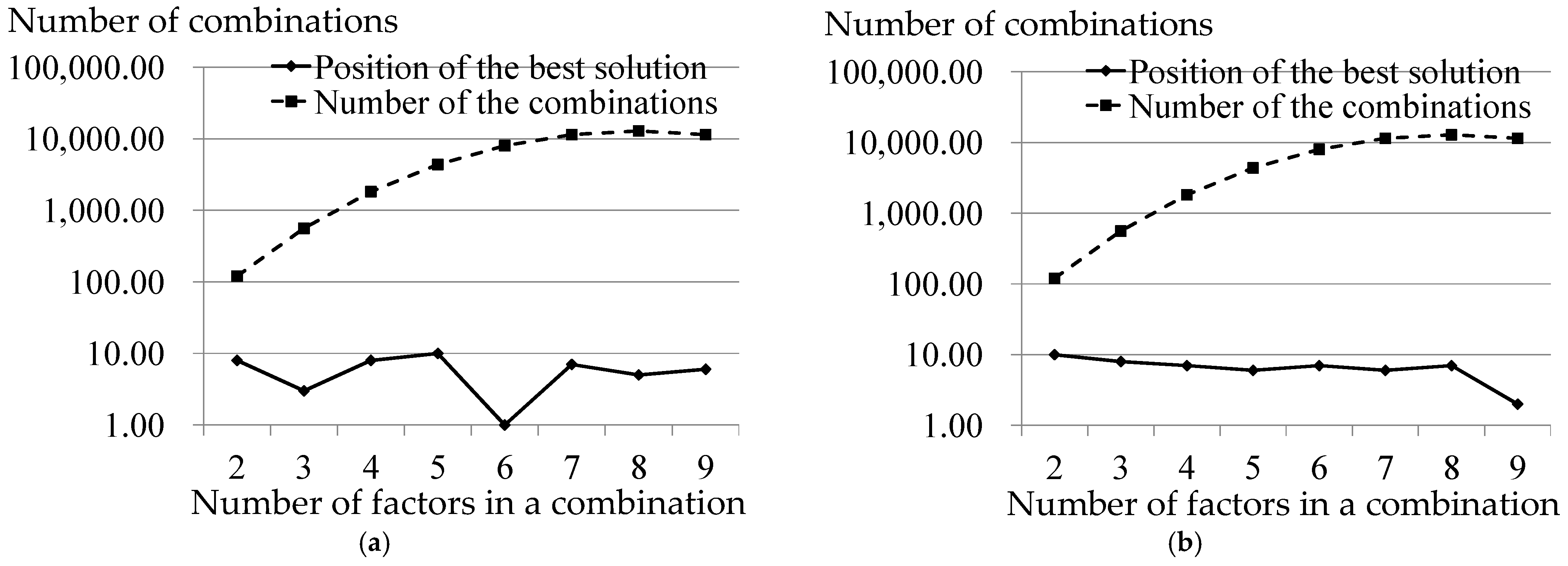
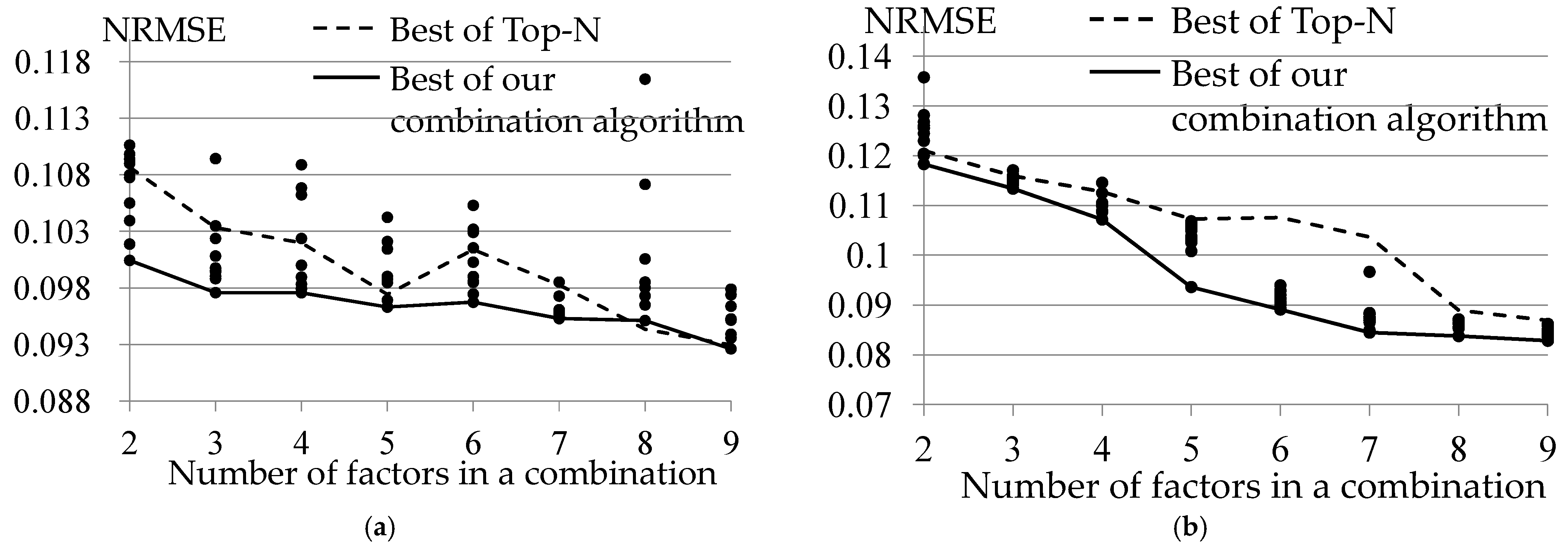
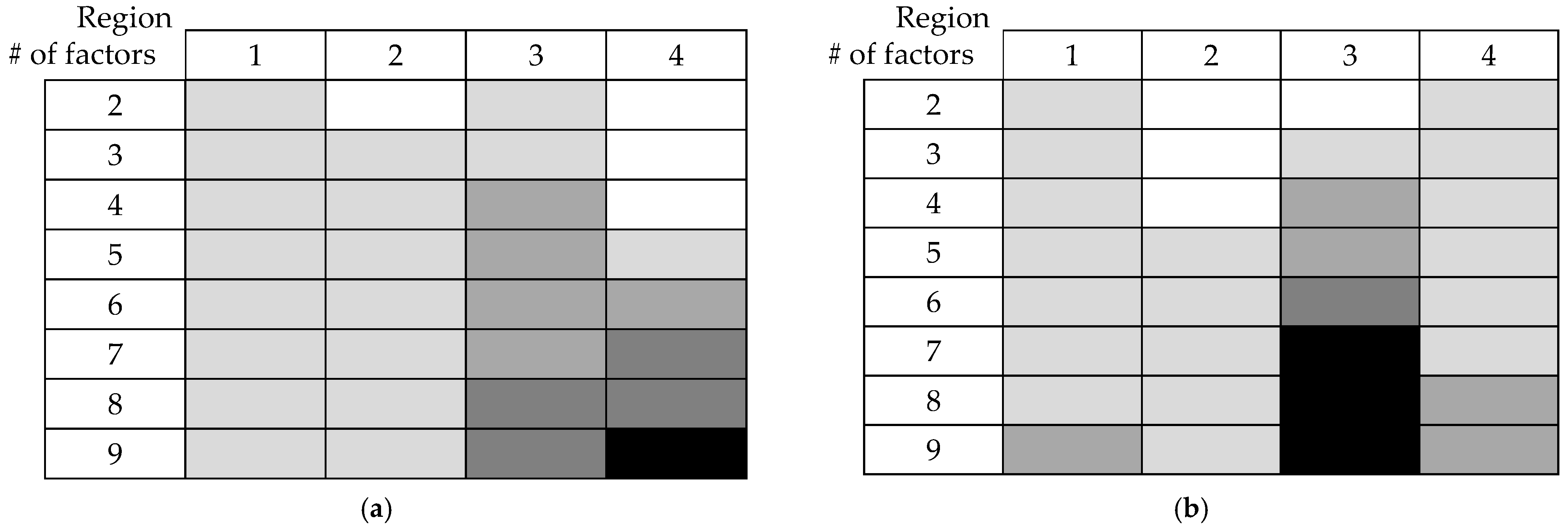
4.4. Verification of Validity of Factor Combination Search Algorithm

Having demonstrated that the trained NC-RBF-DNN is able to derive reasonable importance rankings for all input fields, we next assessed the benefits of the proposed factor combination algorithm in the construction of ensemble effective models based on this ranking. The verification process was implemented into three stages: (1) an examination of the number of combinations that the heap needs to check to find the optimal solution and a comparison, (2) a comparison of the results obtained by the heap and those obtained by the NC-RBF-DNN, and (3) a discussion of the factor combinations used in the optimal solution obtained by the heap.

We use Figure 14 to explore the first part. The x axis in this figure indicates the number of factors in a combination; the solid curve in the figure shows the number of times the heap needs to find a near-optimal solution with combinations containing n factors, and the dashed curve shows the number of combinations with n factors to be found with the 16 factors in our target problem. Due to the massive differences between the values of these two curves, we used a logarithmic scale for the y axis. In Figure 14, we can see that our heap only needs fewer than 10 times to find a near-optimal solution. This is clearly far fewer than the possible number of combinations, thereby demonstrating that the proposed approach can achieve the goal with very little computation.

We next use Figure 15 to look at the prediction errors resulting from the top several combinations in the heap with different number of factors in a combination. The values on the x axis represent the number of factors in a combination, and the multiple dots above each value on the x axis indicate the errors resulting from the top 10 combinations that popped out in the heap with n combinations. Finally, the solid and dashed curves in Figure 15 show the errors generated by the minimum value derived using the heap combination algorithm and the top n combinations obtained using the NC-RBF-DNN. We can observe two phenomena in this figure. The first is that whether we use the lightweight NC-RBF-DNN or the random forest, the minimum errors resulting from the combinations identified using the heap search algorithm were all less than those of modeling with the top several factors identified by the NC-RBF-DNN. This demonstrates the validity of the proposed algorithm. The second phenomenon is that the errors in the results from the top several combinations that popped out in the heap were all lower than those from the ranking derived by the NC-RBF-DNN. This also shows that if we uses the top several combinations identified using the factor combination search algorithm to achieve the ensemble computation for robust prediction, the computation errors of the ensemble model would almost always be lower than or close to those of modeling using the ranking obtained by the NC-RBF-DNN, which also demonstrates that our ensembling results are no poorer than only using a single solution.

Finally, we use Figure 16 to look at the factors that the heap method chose with different numbers of factors in the combinations. The vertical values represent the number of factors in the combinations, and the horizontal values indicate which of the four groups ranked by the NC-RBF-DNN the factors selected by the heap fall in. A deeper color in the grid indicates a higher number of factors selected. From the two sub-graphs in Figure 16, we found that whether the lightweight NC-RBF-DNN or the random forest was used, the heap method chose very few factors from the two first groups; instead, it chose the most factors from the third group and the second most from the fourth group. We speculate that this was because the factors in the first first two groups provided a lot of overlapping information, meaning that for the models, only one factor was needed to establish a model close to the real circumstances. As for the factors in the third group, most only significantly affected solar power generation under special circumstances, so adding them to the model would improve the prediction results of the model in these special circumstances but reduce overall prediction accuracy. Finally, with regard to the factors in the fourth group, the reason they were chosen is similar to that of the third group. However, because their impact on solar power generation is still not very large, the numbers of times they were selected was naturally lower than those for the factors in the third group.

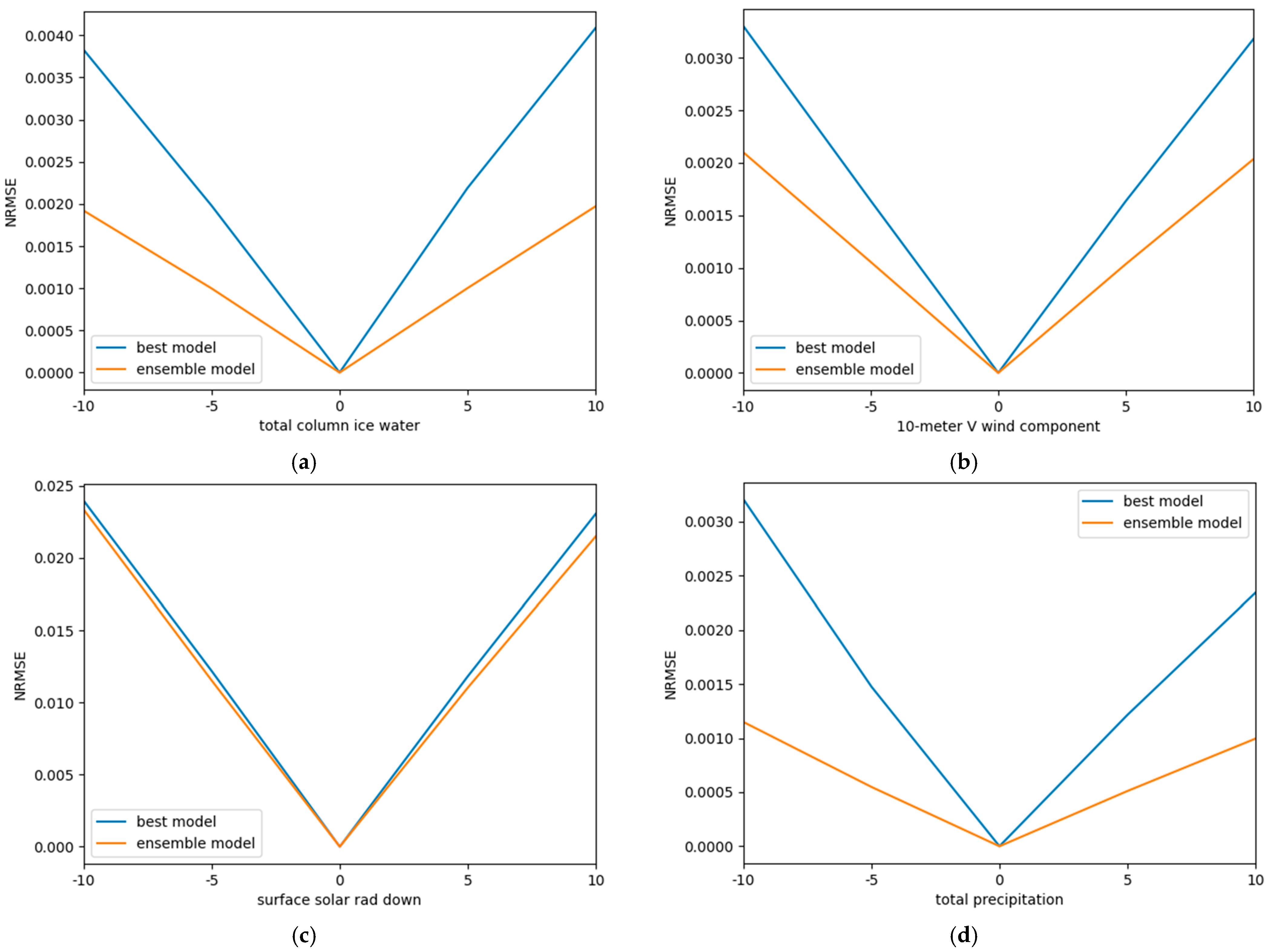
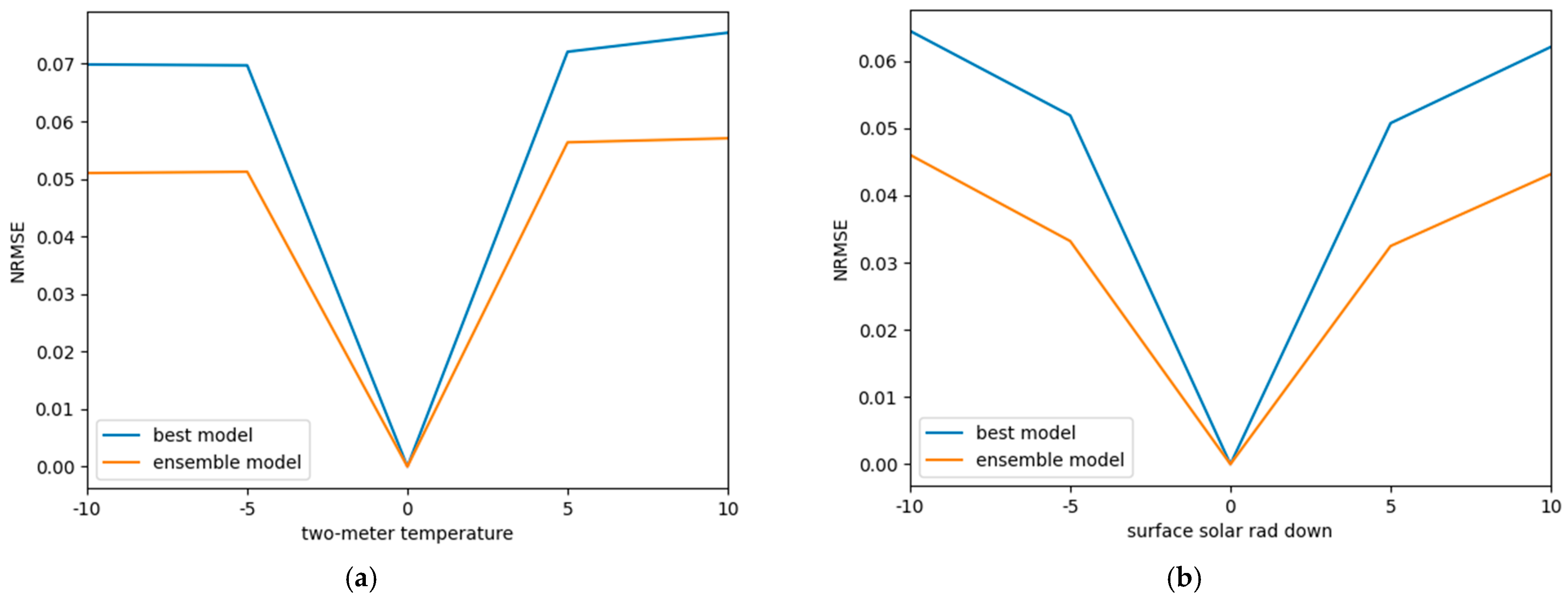
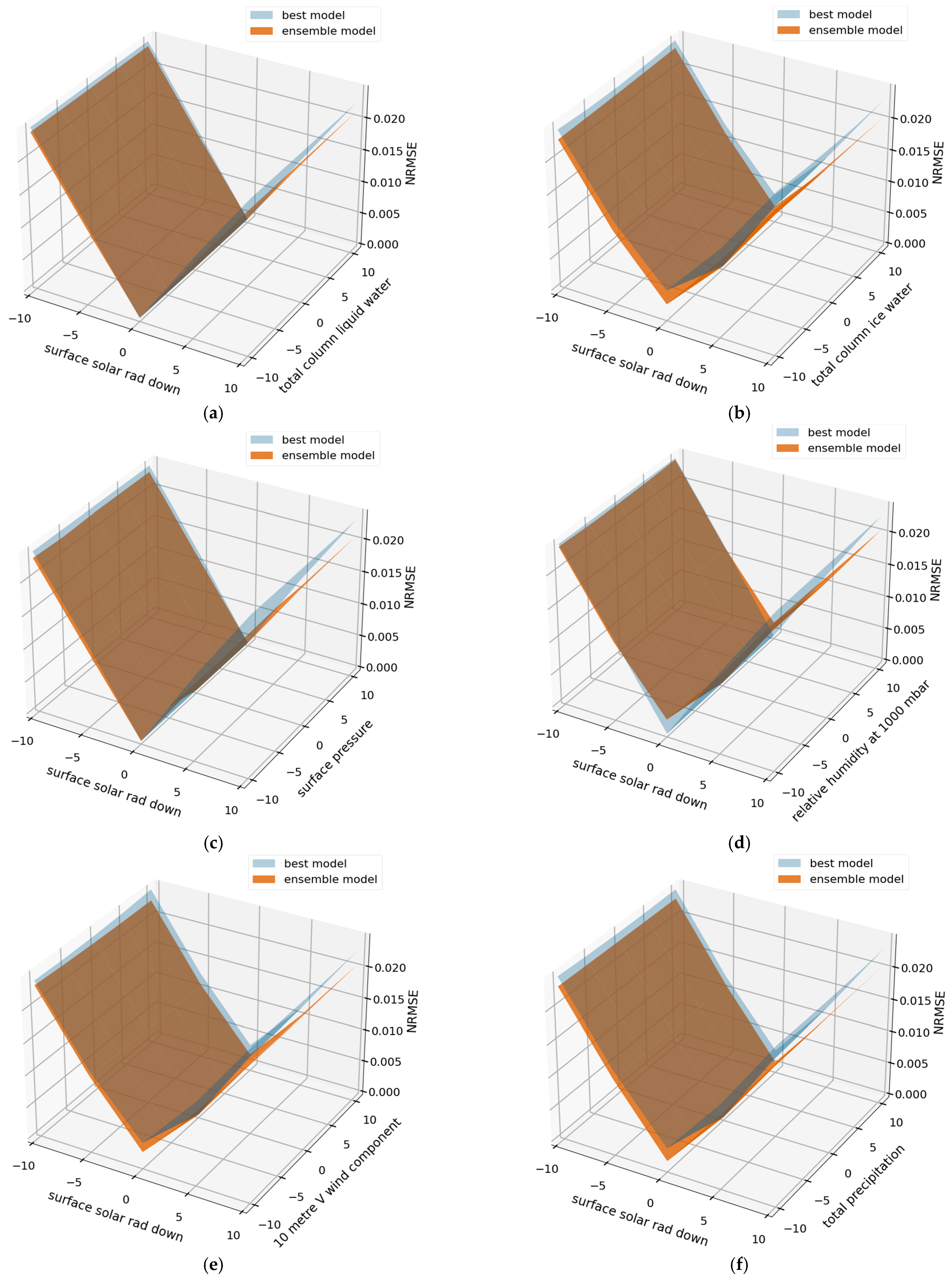
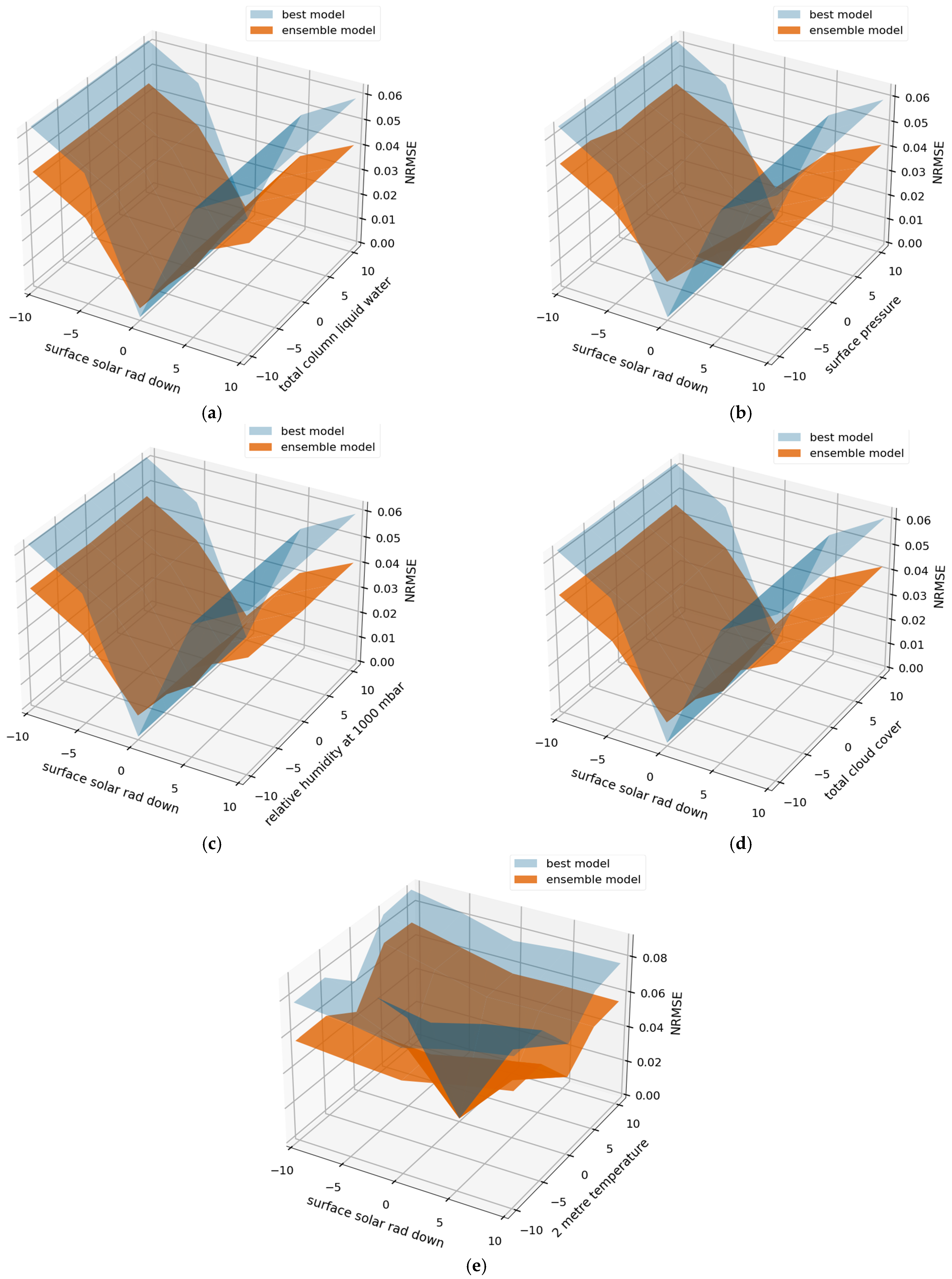
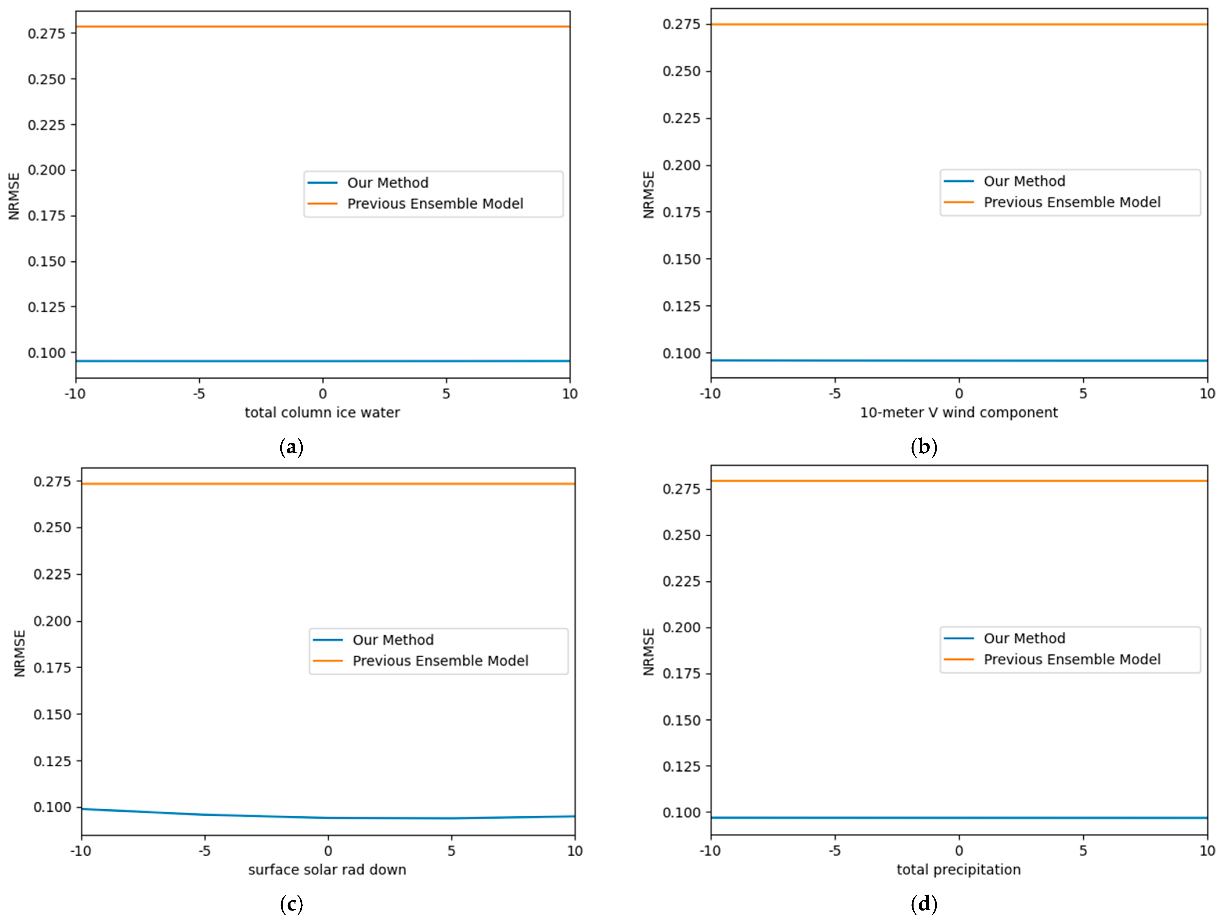
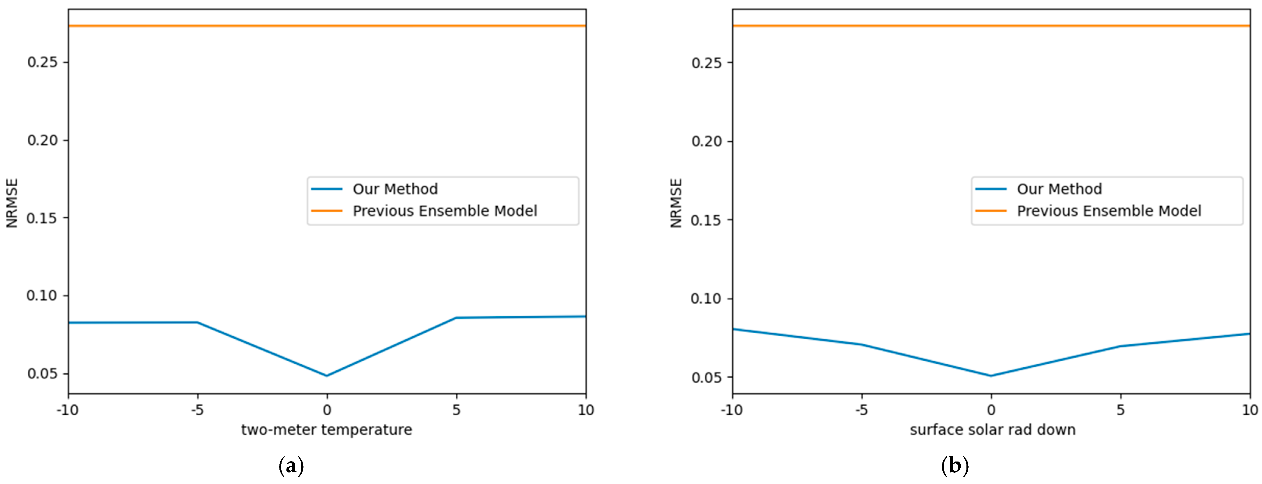
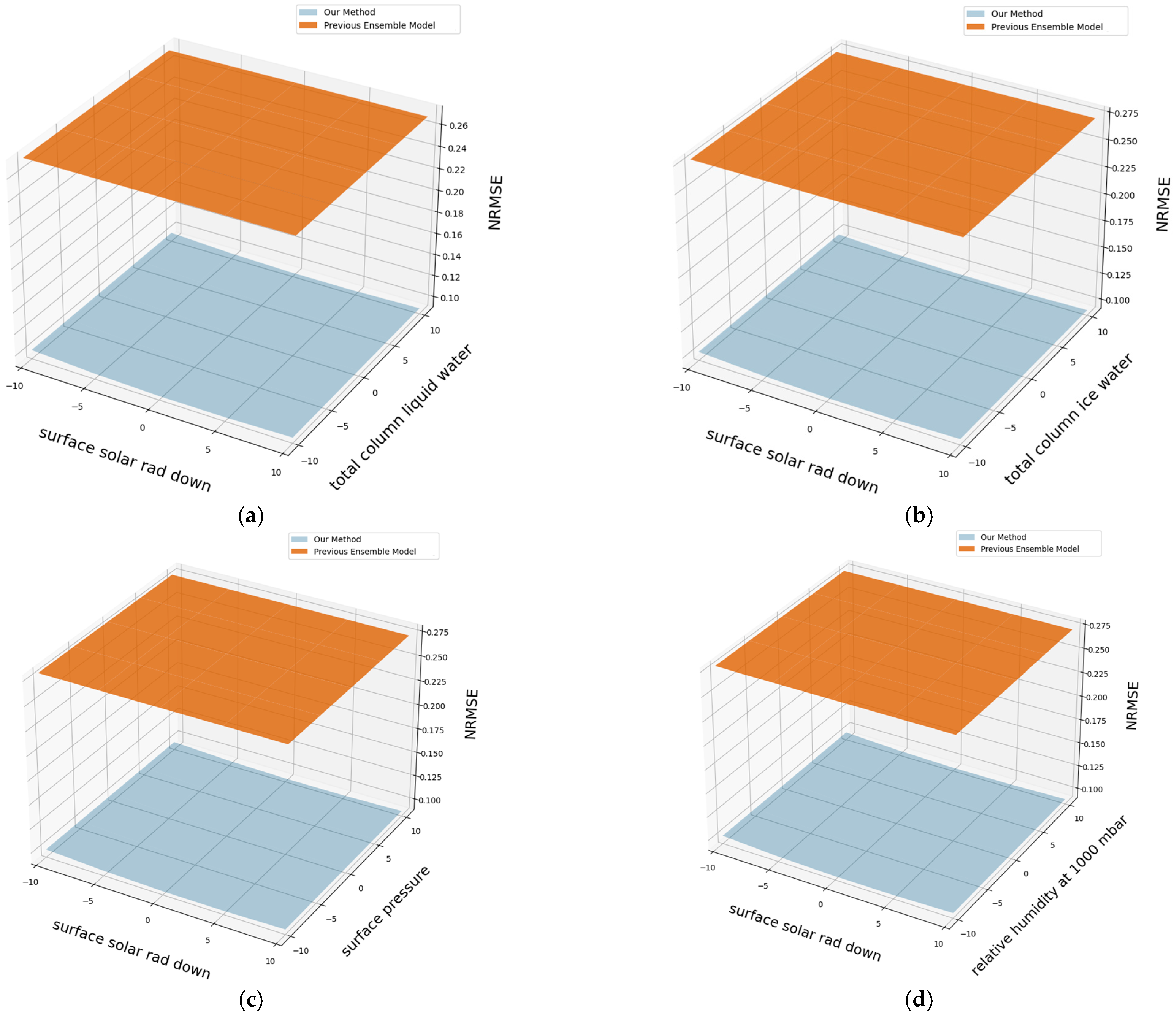
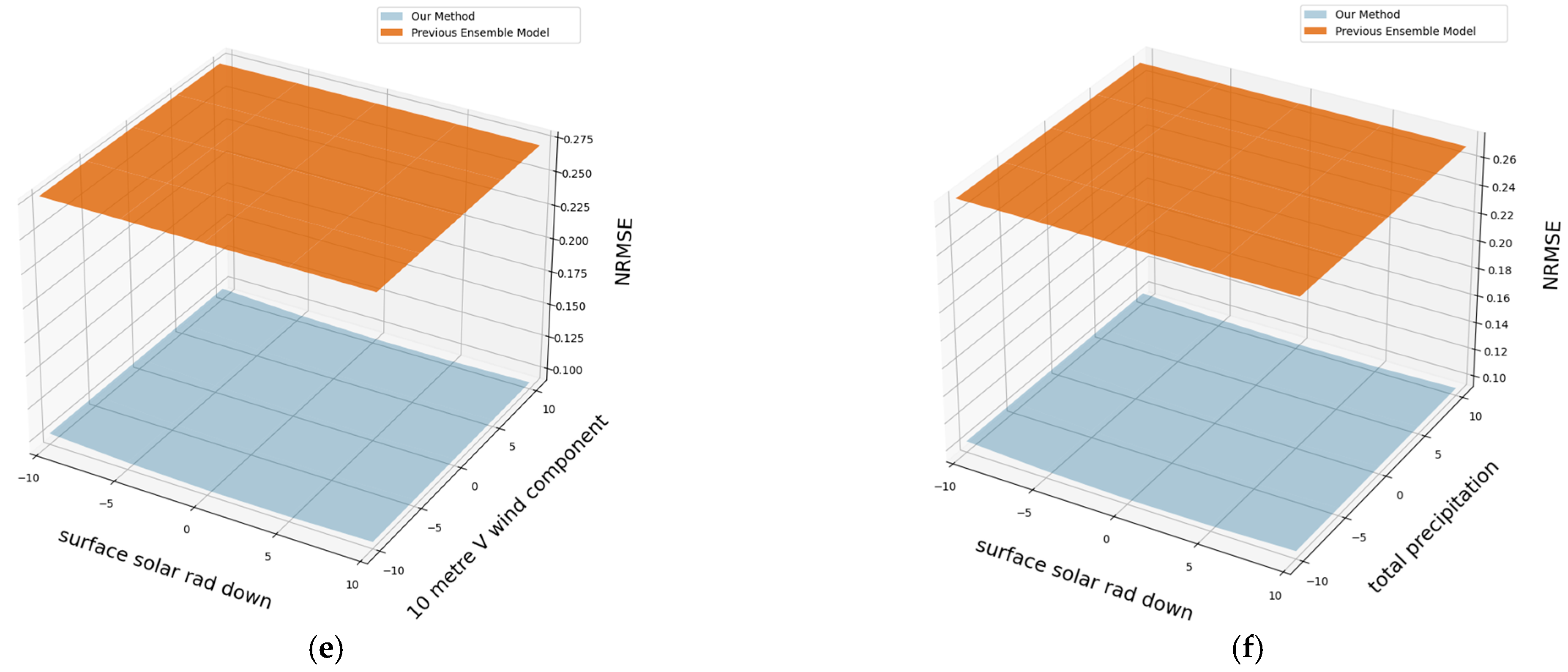
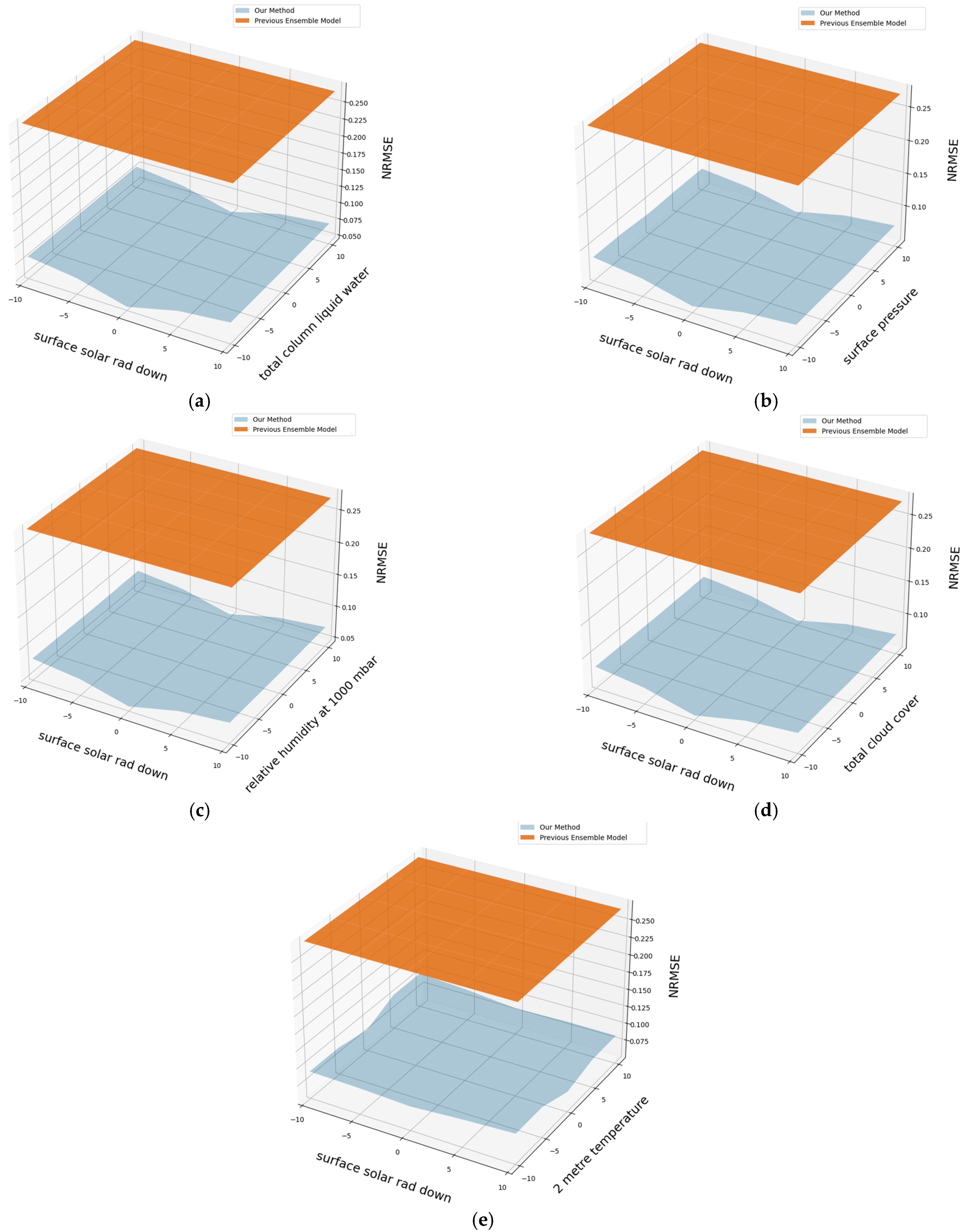
4.5. Performance of Proposed Model with Inputs Containing Errors

In this section, we assess the robustness of the proposed ensemble model in predicting solar power generation. This was achieved by deliberately adding errors at fixed proportions to select weather variables and then inputting all of the fields at time t into the target ensemble model. Finally, we measure the difference between the power generation forecast results at time t and the actual data

We use Figure 17, Figure 18, Figure 19 and Figure 20 to explain how the proposed model achieves robust prediction. In particular, considering that when selecting five factors to combine, both lightweight models can obtain relatively good results, the experiment in this section will be conducted with a combination of five factors. Among them, for lightweight NC-RBF-DNN, its five factors are [total column ice water, 10-m V wind component, surface solar rad down, total precipitation, month] and for random forest, its factors are [Hour, Month, two-meter temperature, surface solar rad down, zone ID]. All three of these figures present the results of two models, including the combination with the minimum error found by the heap method and the average of the five combinations with the smallest errors as determined using the heap method. Furthermore, the −10%, −5%, 0%, 5%, and 10% on the x axes in each graph represent the percentage of error added to or subtracted from certain factors, and the y axes indicate the final output error resulting from the input error. Note that where x equals 0%, there is no error in the input, so naturally the final output error is also 0. Figure 17 and Figure 18 only consider situations where errors only exist in a single factor, which is necessarily used in the optimal model, and errors may occur. Finally, Figure 19 and Figure 20 consider situations where errors exist in two factors, which is necessarily used in the optimal model or ensemble models. In the sub-graphs of these figures, we can clearly see that with either the lightweight NC-RBF-DNN or the random forest, the output errors caused by errors in the input factors of the ensemble model are all less than those of the optimal model, thereby demonstrating that the proposed ensemble model can perform better than a single model.

After completing the comparison with the single best model, we compared the target ensemble model against an existing ensemble model [19]. The comparison model employed a gradient boosting machine, a support vector machine, the random forest algorithm, and the k-nearest neighbor algorithm to train models on the target data set. An ensemble model was then used for model integration. The comparison results in Figure 21, Figure 22, Figure 23 and Figure 24 show that their muti-faceted approach outperformed our simple method in terms of resistance to input error. Nonetheless, the NRMSE of their model was more than ten times higher than that of the proposed method, regardless of the input error combination. Despite the effects of input error, the proposed model achieved output predictions that are closer to the actual results, making it a highly robust solution.

5. Conclusions and Future Works

As green energy technology develops, so too grows research interest in topics such as solar power forecasting. Existing forecasting methods assume the accuracy of input values, which is problematic in practice because errors are inevitable in data collected by sensors. In view of this, we designed a robust solar power forecasting model based on the concepts of ensembling and lightweight deep learning models. In experiments, the proposed method demonstrated the following advantages: (1) In situations without input error, the NRMSE of NC-RBF-DNN in solar power generation prediction was only 0.07874, which is 11.5% better than the typical random forest algorithm. (2) NC-RBF-DNN proved more effective than the Pearson correlation coefficient in assigning model input importance scores, thereby allowing it to skip input factors that are redundant or of low importance to achieve lightweight modeling without sacrificing accuracy. (3) Compared to a prominent existing ensemble model based on four machine learning models, our NC-RBF-DNN ensemble model proved more effective in preventing output errors caused by input errors, as evidenced by ten times lower NRMSE. These experiment results demonstrate the rationale and effectiveness of the proposed method.

In future work, we plan to make the following improvements: (1) establish models for different conditions, such as sunny and rainy days and different seasons, and (2) construct retrainable models. With regard to the first, we discuss in this paper how the importance ranking derived by the NC-RBF-DNN is influenced by whether the factor affects power generation in the long term or the short term. Some important factors with short-term effects are often ranked lower in importance by the NC-RBF-DNN. To overcome this, we plan to deal with normal and special circumstances separately to promote more accurate forecasting. As for the second improvement, it is well known that the prediction accuracy of an artificially intelligent (AI) model gradually decreases with time, so most AI models are trained regularly. However, the proposed model cannot be changed once the input factor combinations have been determined. To make changes, the modeling process must be started from scratch, which is time-consuming and labor-intensive. We therefore hope to adjust this in the future to lighten the burden of retraining.

References

1. Lotfi, M.; Javadi, M.; Osório, G.J.; Monteiro, C.; Catalão, J.P.S. A Novel Ensemble Algorithm for Solar Power Forecasting Based on Kernel Density Estimation. Energies 2020, 13, 216. [Google Scholar] [CrossRef]
2. Bracale, A.; Carpinelli, G.; De Falco, P. A Probabilistic Competitive Ensemble Method for Short-Term Photovoltaic Power Forecasting. IEEE Trans. Sustain. Energy 2017, 8, 551–560. [Google Scholar] [CrossRef]
3. Salinas, L.M.; Jirón, L.A.C.; Rodríguez, E.G. A simple physical model to estimate global solar radiation in the central zone of Chile. In Proceedings of the 24th International Cartographic Conference, Santiago, Chile, 15–21 November 2009; pp. 1–9. [Google Scholar]
4. Diagne, M.; David, M.; Lauret, P.; Boland, J.; Schmutz, N. Review of solar irradiance forecasting methods and a proposition for small-scale insular grids. Renew. Sustain. Energy Rev. 2013, 27, 65–76. [Google Scholar] [CrossRef]
5. Mellit, A.; Massi Pavan, A.; Ogliari, E.; Leva, S.; Lughi, V. Advanced Methods for Photovoltaic Output Power Forecasting: A Review. Appl. Sci. 2020, 10, 487. [Google Scholar] [CrossRef]
6. Boilley, A.; Thomas, C.; Marchand, M.; Wey, E.; Blanc, P. The Solar Forecast Similarity Method: A New Method to Compute Solar Radiation Forecasts for the Next Day. Energy Procedia 2016, 91, 1018–1023. [Google Scholar] [CrossRef]
7. Dambreville, R.; Blanc, P.; Chanussot, J.; Boldo, D. Very short term forecasting of the Global Horizontal Irradiance using a spatio-temporal autoregressive model. Renew. Energy 2014, 72, 291–300. [Google Scholar] [CrossRef]
8. Karteris, M.; Slini, T.; Papadopoulos, A.M. Urban solar energy potential in Greece: A statistical calculation model of suitable built roof areas for photovoltaics. Energy Build. 2013, 62, 459–468. [Google Scholar] [CrossRef]
9. Rahul; Gupta, A.; Bansal, A.; Roy, K. Solar Energy Prediction using Decision Tree Regressor. In Proceedings of the 5th International Conference on Intelligent Computing and Control Systems (ICICCS), Madurai, India, 6–8 May 2021; pp. 489–495. [Google Scholar]
10. Kassim, N.M.; Santhiran, S.; Alkahtani, A.A.; Islam, M.A.; Tiong, S.K.; Mohd Yusof, M.Y.; Amin, N. An Adaptive Decision Tree Regression Modeling for the Output Power of Large-Scale Solar (LSS) Farm Forecasting. Sustainability 2023, 15, 13521. [Google Scholar] [CrossRef]
11. Khalyasmaa, A.; Eronshenko, S.A.; Chakraverthy, T.P.; Gasi, V.G.; Bollu, S.K.Y.; Caire, R.; Atluri, S.K.R.; Karrolla, S. Prediction of Solar Power Generation Based on Random Forest Regressor Model. In Proceedings of the International Multi-Conference on Engineering, Computer and Information Sciences (SIBIRCON), Novosibirsk, Russia, 21–27 October 2019; pp. 780–785. [Google Scholar]
12. Liu, J.; Cao, M.Y.; Bai, D.; Zhang, R. Solar radiation prediction based on random forest of feature-extraction. In Proceedings of the IOP Conference Series: Materials Science and Engineering, Taoyuan, Taiwan, 2–6 November 2018; p. 658012006. [Google Scholar]
13. Reddy, K.S.; Ranjan, M. Solar resource estimation using artificial neural networks and comparison with other correlation models. Energy Convers. Manag. 2003, 44, 2519–2530. [Google Scholar] [CrossRef]
14. Zarzalejo, L.F.; Ramirez, L.; Polo, J. Artificial intelligence techniques applied to hourly global irradiance estimation from satellite-derived cloud index. Energy 2005, 30, 1685–1697. [Google Scholar] [CrossRef]
15. Alam, S.; Kaushik, S.C.; Garg, S.N. Computation of beam solar radiation at normal incidence using artificial neural network. Renew. Energy 2006, 31, 1483–1491. [Google Scholar] [CrossRef]
16. Gensler, A.; Henze, J.; Sick, B.; Raabe, N. Deep Learning for solar power forecasting—An approach using AutoEncoder and LSTM Neural Networks. In Proceedings of the IEEE International Conference on Systems, Man, and Cybernetics (SMC), Budapest, Hungary, 9–12 October 2016; pp. 2858–2865. [Google Scholar]
17. Zhou, H.; Liu, Q.; Yan, K.; Du, Y. Deep Learning Enhanced Solar Energy Forecasting with AI-Driven IoT. Hindawi Wirel. Commun. Mob. Comput. 2021, 1, 9249387. [Google Scholar] [CrossRef]
18. Jamil, I.; Hong, L.; Iqbal, S.; Aurangzaib, M.; Jamil, R.; Hotb, H.; Alkuhayli, A.; AboRas, K.M. Predictive evaluation of solar energy variables for a large-scale solar power plant based on triple deep learning forecast models. Alex. Eng. J. 2023, 76, 51–73. [Google Scholar] [CrossRef]
19. Raj, V.; Dotse, S.-Q.; Sathyajith, M.; Petra, M.I.; Yassin, H. Ensemble Machine Learning for Predicting the Power Output from Different Solar Photovoltaic Systems. Energies 2023, 16, 671. [Google Scholar] [CrossRef]
20. Makasis, N.; Narsilio, G.; Bidarmaghz, A. A robust prediction model approach to energy geo-structure design. Comput. Geotech. 2018, 104, 140–151. [Google Scholar] [CrossRef]
21. Uddin, M.D.; Nash, S.; Diganta, M.T.M.; Rahman, A.; Olbert, A.I. Robust machine learning algorithms for predicting coastal water quality index. J. Environ. Manag. 2022, 321, 115923. [Google Scholar] [CrossRef]
22. Malagutti, N.; Dehghani, A.; Kennedy, R.A. Robust control design for automatic regulation of blood pressure. IET Control Theory Appl. 2013, 7, 387–396. [Google Scholar] [CrossRef]
23. Köhler, J.; Soloperto, R.; Müller, M.A.; Allgöwer, F. A Computationally Efficient Robust Model Predictive Control Framework for Uncertain Nonlinear Systems. IEEE Trans. Autom. Control 2020, 66, 794–801. [Google Scholar] [CrossRef]
24. Pin, G.; Raimondo, D.M.; Magni, L.; Parisini, T. Robust Model Predictive Control of Nonlinear Systems with Bounded and State-Dependent Uncertainties. IEEE Trans. Autom. Control 2009, 54, 1681–1687. [Google Scholar] [CrossRef]
25. Filho, C.M.; Terra, M.H.; Wolf, D.F. Safe Optimization of Highway Traffic With Robust Model Predictive Control-Based Cooperative Adaptive Cruise Control. IEEE Trans. Intell. Transp. Syst. 2017, 18, 3193–3203. [Google Scholar] [CrossRef]
26. Terramanti, T.; Luspay, T.; Kulcsár, B.; Péni, T.; Varga, I. Robust Control for Urban Road Traffic Networks. IEEE Trans. Intell. Transp. Syst. 2014, 15, 385–398. [Google Scholar] [CrossRef]
27. Liu, H.; Claudel, C.G.; Machemehi, R.; Perrine, K.A. A Robust Traffic Control Model Considering Uncertainties in Turning Ratios. IEEE Trans. Intell. Transp. Syst. 2022, 23, 6539–6555. [Google Scholar] [CrossRef]
28. Zhang, C.; Hua, L.; Ji, C.L.; Nazir, M.S.; Peng, T. An evolutionary robust solar radiation prediction model based on WT-CEEDAN and IASO-optimized outlier robust extreme learning machine. Appl. Energy 2022, 322, 119518. [Google Scholar] [CrossRef]
29. Sharma, V.; Yang, D.; Walsh, W.; Reindl, T. Short term solar irradiance forecasting using a mixed wavelet neural network. Renew. Energy 2016, 90, 481–492. [Google Scholar] [CrossRef]
30. Peng, S.; Chen, R.; Yu, B.; Xiang, M.; Lin, X.; Liu, E. Daily natural gas load forecasting based on the combination of long short term memory, local mean decomposition, and wavelet threshold denoising algorithm. J. Nat. Gas Sci. Eng. 2021, 95, 104175. [Google Scholar] [CrossRef]
31. Zhang, K.; Luo, M. Outlier-robust extreme learning machine for regression problems. Neurocomputing 2015, 151, 1519–1527. [Google Scholar] [CrossRef]
32. Torres, M.E.; Colominas, M.A.; Scholtthauer, G.; Flandrin, P. A complete ensemble empirical mode decomposition with adaptive noise. In Proceedings of the IEEE International Conference on Acoustics, Speech and Signal Processing (ICASSP), Prague, Czech Republic, 22–27 May 2011. [Google Scholar]
33. Thorey, J.; Chaussin, C.; Mallet, V. Ensemble Forecast of Photovoltaic Power with Online CRPS Learning. Int. J. Forecast. 2018, 34, 762–773. [Google Scholar] [CrossRef]
34. Zhang, X.; Li, Y.; Lu, S.; Hamann, H.F.; Hodge, B.M.; Lehman, B. A Solar Time Based Analog Ensemble Method for Regional Solar Power Forecasting. IEEE Trans. Sustain. Energy 2019, 10, 268–279. [Google Scholar] [CrossRef]
35. Pan, C.; Tan, J. Day-Ahead Hourly Forecasting of Solar Generation Based on Cluster Analysis and Ensemble Model. IEEE Access 2019, 7, 112921–112930. [Google Scholar] [CrossRef]
36. Hassibi, B.; Stork, D.G. Second order derivatives for network pruning: Optimal brain surgeon. In Proceedings of the Advances in Neural Information Processing Systems, Denver, CO, USA, 29 November–2 December 1993; pp. 164–171. [Google Scholar]
37. Scardapane, S.; Comminiello, D.; Hussain, A.; Uncini, A. Group sparse regularization for deep neural networks. Neurocomputing 2017, 241, 81–89. [Google Scholar] [CrossRef]
38. Wen, W.; Wu, C.; Wang, Y.; Chen, Y.; Li, H. Learning structured sparsity in deep neural networks. In Proceedings of the Advances in Neural Information Processing Systems, Barcelona, Spain, 5–10 December 2016; pp. 2074–2082. [Google Scholar]
39. Han, S.; Pool, J.; Tran, J.; Dally, W. Learning both weights and connections for efficient neural network. In Proceedings of the Advances in Neural Information Processing Systems, Montreal, QC, Cananda, 7–12 December 2015; pp. 1135–1143. [Google Scholar]
40. Li, H.; Kadav, A.; Durdanovic, I.; Samet, H.; Graf, H.P. Pruning filters for efficient convnets. In Proceedings of the International Conference on Learning Representations, Toulon, France, 24–26 April 2017. [Google Scholar]
41. Luo, J.; Wu, J.; Lin, W. ThiNet: A Filter Level Pruning Method for Deep Neural Network Compression. In Proceedings of the IEEE International Conference on Computer Vision, Venice, Italy, 25 December 2017; pp. 5068–5076. [Google Scholar]
42. Molchanov, P.; Tyree, S.; Karras, T.; Aila, T.; Kautz, J. Pruning convolutional neural networks for resource efficient transfer learning. In Proceedings of the International Conference on Learning Representations, Toulon, France, 24–26 April 2017. [Google Scholar]
43. Panchal, G.; Ganatra, A.; Kosta, Y.P.; Panchal, D. Behaviour Analysis of Multilayer Perceptrons with Multiple Hidden Neurons and Hidden Layers. Int. J. Comput. Theory Eng. 2011, 3, 1793–8201. [Google Scholar]
44. Sun, C.; Ma, M.; Zhou, Z.; Tian, S.; Yan, R.; Chen, X. Deep transfer learning based on sparse auto-encoder for remaining useful life prediction on tool in manufacturing. IEEE Trans. Ind. Inform. 2019, 15, 2416–2425. [Google Scholar] [CrossRef]
45. Sani, S.; Wiratunga, N.; Massie, S. Learning deep features for kNN-based human activity recognition. In Proceedings of the International Case-Based Reasoning Conference, Trondheim, Norway, 26–28 June 2017. [Google Scholar]
46. Mohammed, Y.; Matsumoto, K.; Hoashi, K. Deep feature learning and selection for activity recognition. In Proceedings of the Annual ACM Symposium on Applied Computing, New York, NY, USA, 9 April 2018; pp. 930–939. [Google Scholar]
47. Liu, M.; Zhou, M.; Zhang, T.; Xiong, X. Semi-supervised learning quantization algorithm with deep features for motor imagery EEG Recognition in smart healthcare application. Appl. Soft Comput. 2020, 89, 106071. [Google Scholar] [CrossRef]
48. Chen, T.C.; Chang, T.Y.; Chow, H.Y.; Li, S.L.; Ou, C.Y. Using Convolutional Neural Networks to Build a Lightweight Flood Height Prediction Model with Grad-Cam for the Selection of Key Grid Cells in Radar Echo Maps. Water 2022, 14, 155. [Google Scholar] [CrossRef]
49. Jafarpisheh, N.; Zafereni, E.J.; Teshnehlab, M.; Karimipour, H.; Parizi, R.P.; Srivastava, G. A Deep Neural Network Combined with Radial Basis Function for Abnormality Classification. Mobile Netw. Appl. 2021, 26, 2318–2328. [Google Scholar] [CrossRef]
50. Shah, M.H.; Dang, X.Y. Low-complexity deep learning and RBFN architectures for modulation classification of space-time block-code (STBC)-MIMO system. Digit. Signal Process. 2020, 99, 102656. [Google Scholar] [CrossRef]
51. Geng, Z.Q.; Shang, D.R.; Han, Y.M.; Zhong, Y.H. Early warning modeling and analysis based on a deep radial basis function neural network integrating an analytic hierarchy process: A case study for food safety. Food Control 2019, 96, 329–342. [Google Scholar] [CrossRef]
52. Chen, Y.C.; Li, D.C. Selection of key features for PM2.5 prediction using a wavelet model and RBF-LSTM. Appl Intell. 2021, 51, 2534–2555. [Google Scholar] [CrossRef]
53. Chiu, S.M.; Chen, Y.C.; Kuo, C.J.; Hung, L.C.; Hung, M.H.; Chen, C.C. Development of Lightweight RBFDRNN and Automated Framework for CNC Tool-Wear Prediction. IEEE Trans. Instrum. Meas. 2022, 71, 2506711. [Google Scholar] [CrossRef]
54. Chen, Y.C.; Liu, S.C.; Chen, B.X.; Loh, C.H.; Ying, J.C. Ensembling-mRBF-LSTM Framework for Prediction of Abnormal Traffic Flows. In Proceedings of the International Conference on Pervasive Artificial Intelligence, Taipei, Taiwan, 3–5 December 2022; pp. 206–213. [Google Scholar]
55. Chaibi, Y.; Rhafiki, T.E.; Simón-Allué, R.; Guedea, I.; Luaces, C.; Gajate, O.C.; Kousksou, T.; Zeraouli, Y. Physical models for the design of photovoltaic/thermal collector systems. Solar Energy 2021, 226, 134–146. [Google Scholar] [CrossRef]
56. Dolara, A.; Leva, S.; Manzolini, G. Comparison of different physical models for PV power output prediction. Solar Energy 2015, 119, 83–99. [Google Scholar] [CrossRef]
57. Mayer, M.J.; Gróf, G. Extensive comparison of physical models for photovoltaic power forecasting. Appl. Energy 2021, 283, 116239. [Google Scholar] [CrossRef]
58. Kreider, J.; Kreith, F. Solar Energy Handbook; McGraw-Hill: New York, NY, USA, 1981. [Google Scholar]
59. Khatib, T.; Mohamed, A.; Sopian, K. A review of solar energy modeling techniques. Renew. Sustain. Energy Rev. 2012, 16, 2864–2869. [Google Scholar] [CrossRef]
60. Sopian, K.; Othman, M.Y.H. Estimates of monthly average daily global solar radiation in Malaysia. Renew. Energy 1992, 2, 319–325. [Google Scholar] [CrossRef]
61. Chineke, T.C. Equations for estimating global solar radiation in data sparse regions. Renew. Energy 2008, 33, 827–831. [Google Scholar] [CrossRef]
62. Khatib, T.; Mohamed, A.; Mahmoud, M.; Sopian, K. Modeling of Daily Solar Energy on a Horizontal Surface for Five Main Sites in Malaysia. Int. J. Green Energy 2011, 8, 795–819. [Google Scholar] [CrossRef]
63. Iheanetu, K.J. Solar Photovoltaic Power Forecasting: A Review. Sustainability 2022, 14, 17005. [Google Scholar] [CrossRef]
64. Mansoury, I.; Bourakadi, D.E.; Yahyaouy, A.; Boumhidi, J. A novel decision-making approach based on a decision tree for micro-grid energy management. Indones. J. Electr. Eng. Comput. Sci. 2023, 30, 1150–1158. [Google Scholar] [CrossRef]
65. Mellit, A.; Kalogirou, S.A.; Shaari, S.; Salhi, H.; Arab, A.H. Methodology for predicting sequences of mean monthly clearness index and daily solar radiation data in remote areas: Application for sizing a stand-alone PV system. Renew. Energy 2008, 33, 1570–1590. [Google Scholar] [CrossRef]
66. Rajendran, S.S.P.; Gebremedhin, A. Deep learning-based solar power forecasting model to analyze a multi-energy microgrid energy system. Front. Energy Res. 2024, 12, 1363895. [Google Scholar] [CrossRef]
67. Elsaraiti, M.; Merabet, A. Solar Power Forecasting Using Deep Learning Techniques. IEEE Access 2022, 10, 31692–31698. [Google Scholar] [CrossRef]
68. Chang, R.; Bai, L.; Hsu, C.-H. Solar power generation prediction based on deep learning. Sustain. Energy Technol. Assess. 2021, 47, 101354. [Google Scholar] [CrossRef]
69. Sharadga, H.; Hajimirza, S.; Balog, R.S. Times series forecasting of solar power generation for large-scale photovoltaic plants. Renew. Energy 2020, 150, 797–807. [Google Scholar] [CrossRef]
70. Alkandari, M.; Ahmad, I. Solar power generation forecasting using ensemble approach based on deep learning and statistical methods. Appl. Comput. Inform. 2020, 231–250. Available online: https://www.emerald.com/insight/content/doi/10.1016/j.aci.2019.11.002/full/html (accessed on 11 November 2024). [CrossRef]
71. Plessis, A.A.D.; Stauss, J.M.; Rix, A.J. Short-term solar power forecasting: Investigating the ability of deep learning models to capture low-level utility-scale Photovoltaic system behavior. Appl. Energy 2021, 285, 116395. [Google Scholar] [CrossRef]
72. Pedro, H.T.C.; Larson, D.P.; Coimbra, C.F.M. A comprehensive dataset for the accelerated development and benchmarking of solar forecasting methods. J. Renew. Sustain. Energy 2019, 11, 036102. [Google Scholar] [CrossRef]
73. Sun, Y.C.; Venugopal, V.; Brandt, A.R. Short-term solar power forecast with deep learning: Exploring optimal input and output configuration. Solar Energy 2019, 188, 730–741. [Google Scholar] [CrossRef]
74. Paletta, Q.; Arbod, G.; Lasenby, J. Benchmarking of deep learning irradiance forecasting models from sky images—An in-depth analysis. Solar Energy 2021, 224, 855–867. [Google Scholar] [CrossRef]
75. Nie, Y.; Paletta, Q.; Scott, A.; Pamares, L.M.; Arbod, G.; Sgouridis, S.; Lasenby, J.; Brandt, A. Sky image-based solar forecasting using deep learning with heterogeneous multi-location data: Dataset fusion versus transfer learning. Appl. Energy 2024, 369, 123467. [Google Scholar] [CrossRef]
76. Maciel, J.N.; Ledesma, J.J.G.; Ando Junior, O.H. Hybrid prediction method of solar irradiance applied to short-term photovoltaic energy generation. Renew. Sustain. Energy Rev. 2024, 192, 114185. [Google Scholar] [CrossRef]
77. Colak, T.; Qahwaji, R. Automatic Sunspot Classification for Real-Time Forecasting of Solar Activities. In Proceedings of the 3rd International Conference on Recent Advances in Space Technologies, Istanbul, Turkey, 14–16 June 2007; pp. 733–738. [Google Scholar]
78. Monjoly, S.; Andr’e, M.; Calif, R.; Soubdhan, T. Hourly forecasting of global solar radiation based on multiscale decomposition methods: A hybrid approach. Energy 2017, 119, 288–298. [Google Scholar] [CrossRef]
79. Liu, D.; Sun, K. Random forest solar power forecast based on classification optimization. Energy 2019, 187, 115940. [Google Scholar] [CrossRef]
80. Subramanian, E.; Karthik, M.M.; Krishna, G.P.; Prasath, D.V.; Kumar, V.S. Solar power prediction using Machine learning. arXiv 2023, arXiv:2303.07875. [Google Scholar]
81. Roy, S.; Panda, P.; Srinivasan, G.; Raghunathan, A. Pruning Filters while Training for Efficiently Optimizing Deep Learning Networks. In Proceedings of the International Joint Conference on Neural Networks (IJCNN), Glasgow, UK, 19–24 July 2020; pp. 1–7. [Google Scholar]
82. Wu, D.; Lv, S.; Jiang, M.; Song, H. Using channel pruning-based YOLO v4 deep learning algorithm for the real-time and accurate detection of apple flowers in natural environments. Comput. Electron. Agric. 2020, 178, 105742. [Google Scholar] [CrossRef]
83. Chiu, S.-M.; Liou, Y.-S.; Chen, Y.-C.; Lee, Q.; Shang, R.-K.; Chang, T.-Y. Identifying key grid cells for crowd flow predictions based on CNN-based models with the Grad-CAM kit. Appl. Intell. 2022, 53, 13323–13351. [Google Scholar] [CrossRef]
84. Soltani, A.; Meinke, H.; Voil, P.D. Assessing linear interpolation to generate daily radiation and temperature data for use in crop simulations. Eur. J. Agron. 2024, 21, 133–148. [Google Scholar] [CrossRef]
85. Gore, R.; Gawali, B.; Pachpatte, D. Weather Parameter Analysis Using Interpolation Methods. Artif. Intell. Appl. 2023, 1, 260–272. [Google Scholar] [CrossRef]
86. Nagy, G.I.; Barta, G.; Kazi, S.; Borbély, G.; Simon, G. GEFCom2014: Probabilistic solar and wind power forecasting using a generalized additive tree ensemble approach. Int. J. Forecast. 2016, 32, 1087–1093. [Google Scholar] [CrossRef]
87. Barta, G.; Nagy, G.B.G.; Kazi, S.; Henk, T. Gefcom 2014—Probabilistic electricity price forecasting. In Intelligent Decision Technologies. In Proceedings of the 7th KES International Conference on Intelligent Decision Technologies, Sorrento, Italy, 17–19 June 2015; pp. 67–76. [Google Scholar]
88. Hong, T. Energy Forecasting. Available online: http://blog.drhongtao.com/2017/03/gefcom2014-load-forecasting-data.html (accessed on 11 November 2024).
89. Chiu, S.M. The Source Code of RBF-DRNN. Available online: https://github.com/osamchiu/rbf_drnn (accessed on 11 November 2024).
Figure 1. Three existing methods for pruning deep learning model architecture include (1) pruning model weights, (2) pruning entire hidden layers, and (3) pruning unnecessary input factors.
Applsci 14 10625 g001
Figure 2. Flow chart of factor reduction for deep learning architecture pruning.
Applsci 14 10625 g002
Figure 3. Flow chart of proposed methodology.
Applsci 14 10625 g003
Figure 4. Distribution of weather data: (a) normal distribution; (b) data concentrated at minimum value end; (c) data concentrated at minimum and maximum value ends.
Applsci 14 10625 g004
Figure 5. Flow chart of existing lightweight deep learning models during online applications.
Applsci 14 10625 g005
Figure 6. Architecture of proposed NC-RBF-DNN.
Applsci 14 10625 g006
Figure 7. Influence of RBF on numerical values: (a) Scenario 1 when different x values produce different probabilities; (b) Scenario 2 when different x values produce different probabilities; (c) Scenario 1 when different x values produce near-zero probabilities; (d) Scenario 2 when different x values produce near-zero probabilities.
Applsci 14 10625 g007
Figure 8. Influence of RBF on categorical values: (a) Scenario 1 when different x values produce different probabilities; (b) Scenario 2 when different x values produce different probabilities; (c) Scenario 1 when different x values produce near-zero probabilities; (d) Scenario 2 when different x values produce near-zero probabilities.
Applsci 14 10625 g008
Figure 9. Discussion of RBF layer outputs: (a) influencing final model outputs; (b) Scenario 1 when not influencing final model outputs; (c) Scenario 2 when not influencing final model outputs.
Applsci 14 10625 g009
Figure 10. Importance ranking of 16 factors obtained by NC-RBF-DNN and Pearson correlation.
Applsci 14 10625 g010
Figure 11. Comparison of the first 200 normalized values of relative humidity at 1000 mbar, 2 m temperature, and surface solar radiation in the target dataset.
Applsci 14 10625 g011
Figure 12. Comparison of errors resulting from modeling with top n and last n factors: (a) modeling with lightweight NC-RBF-DNN; (b) modeling with random forest.
Applsci 14 10625 g012
Figure 13. Errors resulting from modeling with top n factors.
Applsci 14 10625 g013
Figure 14. Number of combinations that need to be checked for near-optimal solution: (a) modeling with lightweight NC-RBF-DNN; (b) modeling with random forest.
Applsci 14 10625 g014
Figure 15. Prediction errors resulting from top combinations obtained using proposed method and different number of factors in a combination: (a) modeling with lightweight NC-RBF-DNN; (b) modeling with random forest.
Applsci 14 10625 g015
Figure 16. Factors chosen in near-optimal solution with different number of factors in a combination, where the darker the color, the more factors are selected. (a) modeling with lightweight NC-RBF-DNN; (b) modeling with random forest.
Applsci 14 10625 g016
Figure 17. When using lightweight NC-RBF-DNN to model, the impact of one input error on the model output error. (a) Total column ice water, (b) 10-m V wind component, (c) surface solar rad down, (d) total precipitation.
Applsci 14 10625 g017
Figure 18. When using the random forest to model, the impact of one input error on the model output error. (a) Two-meter temperature, (b) surface solar rad down.
Applsci 14 10625 g018
Figure 19. When using lightweight NC-RBF-DNN to model, the impact of two input errors on the model output error. (a) Surface solar rad down vs. total column liquid water, (b) surface solar rad down vs. total column ice water, (c) surface solar rad down vs. surface pressure, (d) surface solar rad down vs. relative humidity at 1000 mbar, (e) surface solar rad down vs. 10 m V wind component, (f) surface solar rad down vs. total precipitation.
Applsci 14 10625 g019
Figure 20. When using the random forest to model, the impact of two input errors on the model output error. (a) Surface solar rad down vs. total column liquid water, (b) surface solar rad down vs. surface pressure, (c) surface solar rad down vs. relative humidity at 1000 mbar, (d) surface solar rad down vs. total cloud cover, (e) surface solar rad down vs. 2 m temperature.
Applsci 14 10625 g020
Figure 21. Comparison of NRMSE between our ensemble lightweight NC-RBF-DNN and previous models [19] when an input error is present. (a) Total column ice water, (b) 10-m V wind component, (c) surface solar rad down, (d) total precipitation.
Applsci 14 10625 g021
Figure 22. Comparison of NRMSE between our ensemble random forest and previous models [19] when an input error is present. (a) Two-meter temperature, (b) surface solar rad down.
Applsci 14 10625 g022
Figure 23. Comparison of NRMSE between our ensemble lightweight NC-RBF-DNN and previous models when two input errors are present. (a) Surface solar rad down vs. total column liquid water, (b) surface solar rad down vs. total column ice water, (c) surface solar rad down vs. surface pressure, (d) surface solar rad down vs. relative humidity at 1000 mbar, (e) surface solar rad down vs. 10 m V wind component, (f) surface solar rad down vs. total precipitation.
Applsci 14 10625 g023aApplsci 14 10625 g023b
Figure 24. Comparison of NRMSE between our ensemble random forest and previous models when two input errors are present. (a) Surface solar rad down vs. total column liquid water, (b) surface solar rad down vs. surface pressure, (c) surface solar rad down vs. relative humidity at 1000 mbar, (d) surface solar rad down vs. total cloud cover, (e) surface solar rad down vs. 2 m temperature.
Applsci 14 10625 g024