Impact of Feature Selection Techniques on the Performance of Machine Learning Models for Depression Detection Using EEG Data

Abstract

Major depressive disorder (MDD) poses a significant challenge in mental healthcare due to difficulties in accurate diagnosis and timely identification. This study explores the potential of machine learning models trained on EEG-based features for depression detection. Six models and six feature selection techniques were compared, highlighting the crucial role of feature selection in enhancing classifier performance. This study investigates the six feature selection methods: Elastic Net, Mutual Information (MI), Chi-Square, Forward Feature Selection with Stochastic Gradient Descent (FFS-SGD), Support Vector Machine-based Recursive Feature Elimination (SVM-RFE), and Minimal-Redundancy-Maximal-Relevance (mRMR). These methods were combined with six diverse classifiers: Logistic Regression, Support Vector Machine (SVM), Random Forest, Extreme Gradient Boosting (XGBoost), Categorical Boosting (CatBoost), and Light Gradient Boosting Machine (LightGBM). The results demonstrate the substantial impact of feature selection on model performance. SVM-RFE with SVM achieved the highest accuracy (93.54%) and F1 score (95.29%), followed by Logistic Regression with an accuracy of 92.86% and F1 score of 94.84%. Elastic Net also delivered strong results, with SVM and Logistic Regression both achieving 90.47% accuracy. Other feature selection methods yielded lower performance, emphasizing the importance of selecting appropriate feature selection and machine learning algorithms. These findings suggest that careful selection and application of feature selection techniques can significantly enhance the accuracy of EEG-based depression detection.

1. Introduction

Major depressive disorder (MDD) is a complex and serious mental illness that affects millions of people worldwide. The disorder goes beyond typical mood fluctuations and can lead to significant impairment in social, occupational, and educational aspects of life. MDD is a prevalent mental health condition that encounters substantial hurdles in achieving a precise diagnosis. In addition, the underlying causes and development of depression remain poorly understood.

Physicians and psychiatrists traditionally diagnose depression using clinical questionnaires, such as the Beck Depression Inventory or the Patient Health Questionnaire, that rely on patient responses and behavioral observations. However, this approach is subjective, making it difficult to diagnose MDD accurately and objectively. Extensive research has been done to improve the reliability of this traditional method and explore alternative diagnostic strategies. Various techniques have emerged, such as visual assessment of facial expressions, Heart Rate Variability (HRV) analysis, Magnetic Resonance Imaging (MRI), emotional analysis, acoustic properties of speech, and analysis of social media posts. However, some of these methods have limitations, such as the need for long-term and close monitoring in visual evaluation, the sensitivity of HRV analysis to external factors, and the high cost of MRI [1]. The other approach gaining attention is using Electroencephalography (EEG), which records brain electrical activity. Given depression’s neurological impact, researchers worldwide are actively seeking improved EEG-based biomarkers for diagnosis. Recent studies have shown that EEG-based depression detection is a promising new approach because EEG is less complex, more cost-effective, and more patient-friendly than MRI [2].

Machine and deep learning models [3] show promise for improving depression detection, yet several important challenges must be addressed before they can be widely used. One challenge is ensuring the quality of the data used to train these models. It is crucial to use diverse and reliable data. Another challenge is model interpretability—patients and doctors should understand how these models make predictions. Additionally, addressing biases in these models is essential, as biased results may lead to incorrect diagnoses.

Despite these challenges, machine learning has the potential to revolutionize the way that depression is detected and diagnosed. With further research and development, machine learning models could be used to improve early detection of depression and lead to better treatment outcomes.

This research addresses a significant challenge in mental healthcare, depression detection, emphasizing the need for a more objective, data-driven approach. By exploring the potential of machine learning models trained on EEG-based features, this study compares six models and six feature selection techniques. The primary contribution lies in a comprehensive evaluation of these feature selection techniques across the models, providing critical insights into the relationship between feature selection and model performance, particularly in the context of EEG-based depression detection. This research highlights the critical role of feature selection in optimizing classifier performance, even with hyperparameter tuning, furthering the field of EEG-based depression detection and underlining the importance of meticulous feature selection for maximizing model effectiveness.

This paper is organized into key sections as follows: the Background section introduces the existing state of the field. In the Methodology section, the research approach is detailed, including explanations of the dataset, preprocessing steps, and the feature selection techniques used. The Models section discusses the machine learning models and their hyperparameter tuning. Evaluation Metrics are explained to clarify the chosen assessment criteria. The Results section presents the outcomes of the experiments, and the paper concludes with the Conclusion and Future Work section, summarizing findings and proposing future research directions.

The contributions of this paper are as follows:

• A comprehensive evaluation of feature selection techniques across multiple models: This study offers a systematic comparison of six feature selection techniques across various machine learning models. By evaluating models with and without feature selection, it demonstrates the substantial impact these techniques have on classifier performance, especially for high-dimensional EEG data.
• Insights into the differential impact of feature selection on linear and non-linear models: The findings reveal that feature selection techniques influence linear and non-linear models differently. Methods like RFE and Elastic Net enhance linear models by reducing feature redundancy, while techniques such as MI and mRMR are more effective for non-linear models that rely on capturing complex interactions.
• Identification of effective combinations of feature selection techniques and classifiers: This study identifies promising combinations of feature selection methods and classifiers, showing how targeted feature selection can narrow the performance gap between simpler models and more complex approaches, especially in high-dimensional EEG datasets.
• Impact on clinical diagnostics and computational neuroscience: By demonstrating the crucial role of feature selection in optimizing model performance, this research provides valuable insights that could advance clinical diagnostics and computational neuroscience. It supports the development of more accurate and interpretable machine learning models for depression detection, contributing to better diagnostic tools for mental health.

2. Background

In general, the field of Affective Computing has shown significant interest in using physiological cues to assess emotional states [4]. Some psychological and physiological research has suggested a connection between physiological processes and the way we perceive emotions. Therefore, Computational Psychophysiology-based approaches are seen as valuable additions to recognition methods that rely on non-physiological cues like facial expressions or speech. These non-physiological cues can be less reliable, especially when individuals intentionally conceal their true emotions. Given that the brain regulates the autonomic nervous system during emotional experiences, exploring the use of brain activity information, such as EEG, to understand emotional cognition mechanisms and detect emotional states is a particularly promising area of study [5].

Research has shown a direct connection between the central nervous system and emotional processes. EEG serves as an external indicator of the brain’s cognitive psychological functions, making it a valuable tool for studying emotional psychology and developing emotion-recognition technology. However, it is important to construct recognition models that include EEG data from all significant frequency bands and cortex regions, as described by [6].

EEG-based emotion recognition is a subset of pattern-recognition research, and it follows a structured process to address recognition challenges [5]. In pattern recognition, several fundamental steps are involved. First, there is the essential task of defining and quantifying the recognition goal, transforming it into a computable problem. Second, obtaining high-quality research data is crucial because it forms the basis for effectively defining models’ decision boundaries. Third, data preprocessing and representation, including feature extraction or feature learning, play an essential role in building pattern recognition models. These steps ensure that relevant characteristics are extracted from raw data while eliminating extraneous information. Finally, the iterative process of designing, training, and evaluating recognition models based on processed data continues until an acceptable level of recognition accuracy is achieved. EEG-based emotion recognition uses this structured approach to understand emotional states from brainwave data [7].

Multiple studies have emphasized the significance of frequency domain attributes and functional connectivity (FC) in identifying depression using resting-state Electroencephalography (rsEEG) [8,9]. Studying rsEEG features has the potential to reveal complex neural mechanisms associated with depression. The rise of computational psychiatry has amplified interest in using rsEEG-based machine learning methods to identify disease patterns, laying a foundation for clinical depression diagnosis [10].

As described by [11], mental disorders like depression and bipolar disorder can cause the body to release cortisol, a stress hormone, into the brain. Cortisol can affect the production and communication of neurons, which can slow down the function of certain parts of the brain and change the electrical activity patterns. The voltage variations resulting from ionic current flows within the neurons of the brain may be useful for diagnosing mental disorders such as depression and bipolar disorder. According to [12], the amplitude of brain responses (ABR) in the central, frontal, and parietal regions could potentially serve as biomarkers for differentiating patients with depression from healthy individuals.

Brain activity changes when brain function deteriorates, which can be detected using EEG brain scans. EEG is a valuable tool due to its affordability, accessibility, and high temporal resolution, allowing measurement of brain activity in milliseconds. However, EEG signals are complex, non-stationary, and non-linear, which makes manual interpretation challenging. Automated signal-processing techniques enable the accurate classification of individuals with depression compared to those without.

Developing reliable methods for analyzing brain signals is difficult because they are complex, unstructured, and vary greatly depending on the person, their age, and their mental health. Furthermore, EEG recordings can be affected by extraneous noise from eye blinking and muscle movements. These artifacts can obscure the underlying neural activity, hindering the ability to accurately interpret the EEG data. Therefore, it is crucial to distinguish the relevant neural signals from the background noise and artifacts that occur during EEG recordings [13,14].

To address this challenge, a robust and consistent EEG preprocessing method is essential. EEG data preprocessing encompasses a procedure to transform raw EEG data into a refined format by eliminating unwanted noise and artifacts, making it suitable for further analysis and user interpretation [15].

In the field of EEG signal classification, various methods have been proposed to enhance the accuracy and efficiency of the process. For instance, a method was proposed using pattern recognition and a Support Vector Machine (SVM) optimized by an Improved Squirrel Search Algorithm (ISSA) [16]. This method involves extracting time-domain features, applying an elliptical filter to isolate specific frequency bands, and utilizing a multichannel weighted Wiener filter for artifact reduction. Another approach was developed to anticipate individual dynamic ranges of EEG features, facilitating personalized calibration and improving overall performance [17]. These studies highlight the ongoing efforts to refine EEG signal-processing techniques for various applications.

Additionally, EEG signals introduce complexities into the feature extraction and signal analysis process due to their non-stationary nature (with statistics change over time), non-linear behavior, and non-Gaussian distribution [18]. These unique properties must be considered and accommodated in the feature extraction process to establish a robust end-to-end pipeline. EEG signals can be categorized based on location, amplitude, frequency, morphology, continuity, synchrony, symmetry, and reactivity. The most common classification is based on frequency bands, with each band exhibiting unique characteristics and associations with various brain states. EEG patterns can be analyzed by dividing them into frequency ranges, with each range corresponding to specific patterns and brain activities. Commonly studied waveforms include delta (0.5–4 Hz), theta (4–7 Hz), alpha (8–12 Hz), sigma (12–16 Hz), and beta (13–30 Hz). Additional waveforms like infra-slow oscillations (ISO) and high-frequency oscillations (HFOs) have clinical relevance.

EEG, which captures detailed neural electrical activity, provides valuable insights. The correlation between different brain regions proves crucial in depression detection, complementing the distinctive characteristics of individual channels. The growing interest in using EEG data for diagnosing depression has driven innovative research aimed at improving feature selection and classification approaches. Resting-state and sound-stimulated EEG data were analyzed in [19], where minimal-redundancy-maximal-relevance (mRMR) was employed for feature selection alongside the k-nearest neighbor classifier. In [20], L1-based, tree-based, and false discovery rate (FDR) feature selection methods were utilized along with various machine learning models, including SVM, KNN, decision tree, Naïve Bayes, Random Forest, and Logistic Regression. Feature selection based on ranking features using the receiver operating characteristics (ROC) criterion in descending order was conducted in [21], followed by selecting subsets containing the top-ranked features. The classifiers used included Logistic Regression (LR), the Support Vector Machine (SVM), and Naïve Bayesian (NB). The performance of the SVM on different EEG features was explored in [22].

Most existing approaches rely on a single feature selection technique across different classifiers, which can limit the model’s ability to fully capture the complexity of EEG data. This approach may overlook important features that could improve classification accuracy. For example, while mRMR aims to reduce redundancy and maximize relevance, it might miss non-linear relationships between features. Similarly, ROC-based ranking could focus on features with high individual performance but neglect the collective importance of feature combinations. This might result in a feature set that is not optimal for all classifiers, potentially affecting both the overall performance and generalizability of the model. Although the importance of feature selection is widely acknowledged in machine learning, the effects of different feature selection techniques on specific classification models for EEG data, particularly in terms of accuracy, false positives, and false negatives, remain an area of ongoing investigation.

Therefore, this paper presents a study aimed at addressing the limitations of previous research by investigating the impact of a range of feature selection techniques—filter-based, wrapper-based, and embedded methods—on the performance of several machine learning models. By systematically experimenting with techniques such as Elastic Net and SVM-RFE and applying them to classifiers like Logistic Regression and the SVM, this study identifies the most effective combinations and explores the impact of feature selection techniques on classifiers’ performance. The findings highlight the importance of carefully selecting and testing feature selection methods and classifiers, which could lead to more accurate and reliable results.

3. Methodology

This section is structured into several subsections that describe the dataset and data preprocessing details, followed by feature selection classification and techniques used in this study. Then, selected models are briefly discussed, including their hyperparameter tuning.

3.1. Dataset and Preprocessing

In this work, an open-access EEG dataset provided by [23] was adopted to evaluate the performance of multiple machine learning algorithms. This study uses a subset of the dataset from [23], focusing solely on depressive disorder, whereas the original dataset includes multiple psychiatric disorders. The dataset includes preprocessed EEG data for 95 healthy controls (HCs) and 199 with depressive disorder. Data were collected retrospectively from medical records, psychological assessment batteries, and quantitative EEG (QEEG) at resting-state assessments from January 2011 to December 2018 from the Seoul Metropolitan Government-Seoul National University (SMG-SNU) Boramae Medical Center in Seoul, South Korea.

The EEG signals were preprocessed using the NG Deluxe 3.0.5 system, involving several steps. First, the data underwent down-sampling to 128 Hz. The baseline EEG was then identified by applying a filtering process at <1 Hz and >40 Hz using 5th order Butterworth filters. The spliced selections of EEG were filtered a second time with the same parameters after finding the baseline EEG. NeuroGuide utilized a splicing method to append edited selections of EEG, followed by baselining using Butterworth high-pass and low-pass filters at 1 Hz and 55 Hz, respectively [23]. Subsequently, 19 channels with the linked-ear reference were selected for analysis based on the International 10–20 System.

Artifacts, such as those from eye blinks, movements, and drowsiness, were eliminated through visual inspection and the NG Deluxe 3.0.5 cleaning system. Continuous EEG data were then transformed into the frequency domain using Fast Fourier Transformation (FFT) with specific parameters, including an epoch of 2 s, a sample rate of 128 samples/s, and a frequency range of 0.5–40 Hz [23]. A minimum epoch length of 60 s was chosen to address noise in the FFT results. Frequency bands were as follows: beta (12–30 Hz), alpha (8–12 Hz), theta (48 Hz), and delta (0.5–4 Hz). A total of 19 of the 64 channels with the linked-ear reference were selected for the analysis based on the international 10–20 system: FP1, FP2, F7, F3, Fz, F4, F8, T3, C3, Cz, C4, T4, T5, P3, Pz, P4, T6, O1, and O2, as shown in Figure 1 (developed using MNE-Python).

The calculation of each EEG parameter was performed within specific frequency bands: delta (1–4 Hz), theta (4–8 Hz), alpha (8–12 Hz), beta (12–25 Hz), high beta (25–30 Hz), and gamma (30–40 Hz). Power spectral density (PSD) represents the actual spectral power measured at the sensor level. It quantifies the power of different frequency components of the EEG signal. The absolute power value was extracted for each frequency band. Functional connectivity (FC) was quantified using coherence, a measure of synchronization between two signals based on phase consistency [23]. FC is the strength to which activity between a pair of brain regions covaries or correlates over time. The decision to use only PSD and FC as features for depression detection using EEG is based on their strong relevance to the neurophysiological mechanisms underlying depression. Both PSD and FC offer insights into brain activity and connectivity patterns, which are crucial for understanding mood disorders. Research indicates that individuals with depression often show increased theta activity and decreased alpha activity [24,25]. By focusing on PSD, the model can capture these frequency-specific changes. Additionally, disrupted FC patterns, particularly within networks like the Default Mode and Executive Control Networks, have been observed in depressed individuals [26]. Alterations in FC are linked to cognitive dysfunctions seen in depression, such as impaired attention and executive function [27]. Additionally, both features are more robust to noise in EEG signals, offering better stability compared to raw time-domain data [28].

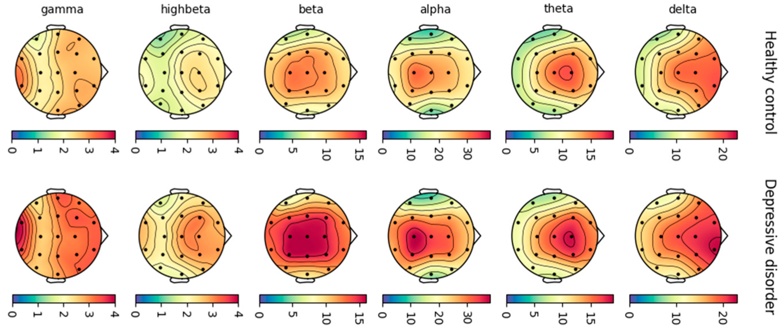
Figure 2 presents topoplots visualizing the average PSD of EEG activity for different frequency bands (delta, theta, alpha, etc.) in healthy controls and individuals with depression. The topoplots were generated using MNE-Python.

3.2. Feature Selection

Feature selection plays a crucial role in enhancing classification performance. Often characterized as an NP-hard combinatorial problem due to the exponential growth of potential feature subsets, it requires careful selection of a significant subset for optimal model building. Relying on independent features is crucial for successful performance in statistical techniques. Therefore, selecting informative and non-redundant features becomes the primary goal of feature selection algorithms [24].

Feature selection is a commonly used technique to reduce the dimensionality of a dataset. It involves four main steps: generating a feature subset, evaluating it, checking termination conditions, and validating results. Feature selection methods can be supervised, unsupervised, or semi-supervised. Categorized by selection strategy, feature selection methods fall into three main types: filter, wrapper, and embedded.

Filter methods rely on intrinsic data properties, independent of any learning algorithm. They employ ranking and scoring techniques to select features based on criteria like discriminative power or correlation with the target variable. Filter methods are fast and flexible but may not be optimal for specific algorithms.

Wrapper methods use prediction models to thoroughly search for the best subsets of predictors. They iteratively refine the selection based on the model’s performance, ensuring that chosen features optimize prediction. While effective, wrapper methods are computationally intensive due to the large search space.

Embedded methods strike a balance between filter and wrapper methods by integrating feature selection into the algorithm’s training process. It balances the speed of filter methods with the accuracy of wrappers [25,26].

This section presents a comparative analysis of established feature selection techniques frequently utilized in the domains of emotion recognition and depression detection using EEG signals. Selecting features is a crucial aspect of designing expert systems, particularly in supervised learning.

The processed dataset comprises 1140 candidate features, 114 PSD and 1026 FC, as follows. Features were extracted from each frequency band individually, including delta, theta, alpha, beta, high beta, and gamma. Additionally, features were extracted from all six bands combined. Demographic and cognitive factors such as age, sex, education, and IQ were considered as additional features. The number of features used in the models ranged from 19-channel PSD in the delta band to 1140 [(19-channel PSD + 171 pair FC) × all six bands]. This wide range reflects the flexibility in feature selection for EEG-based classification.

Various research methodologies have explored training and testing models using combinations of PSD bands and functional connectivity (FC) features in EEG-based machine learning applications, such as Delta PSD + FC. Notably, performance outcomes are often superior when features are selected from both PSD and FC [29].

Combining PSD and FC provides a more comprehensive representation of brain activity. While PSD measures the intensity of brain oscillations, FC reveals connectivity between brain regions. This dual approach enhances the model’s ability to differentiate between depressed and non-depressed states.

In this study, six feature selection approaches were examined: (1) Elastic Net, (2) Mutual Information (MI), (3) Chi-Square, (4) Forward Feature Selection with Stochastic Gradient Descent (FFS-SGD), (5) Support Vector Machine-based Recursive Feature Elimination (SVM-RFE), and (6) Minimal-Redundancy-Maximal-Relevance (mRMR).

Table 1. Feature selection methods.

Filter	Wrapper	Embedded
Mutual Information (MI)	Forward Feature Selection (FFS)	Elastic Net-Based
Chi-square	Support Vector Machine-based Recursive Feature Elimination (SVM-RFE)
Minimal-Redundancy-Maximal-Relevance (mRMR)

summarizes the feature selection methods used in this study, categorizing them into filter, wrapper, and embedded approaches based on their underlying techniques.

For each feature selection technique, the optimal number of features was determined through a systematic process that involved testing various feature sets, starting from the top 100 features and incrementing by 100 up to the top 500 features. This range was chosen to address the challenges associated with high-dimensional EEG data, which can complicate data analysis and increase computational demands. The selection of the top 100 features was found to be optimal, balancing classification performance with computational efficiency. Furthermore, this systematic evaluation allowed for a comprehensive assessment of model performance across different feature configurations, reinforcing the effectiveness of the chosen feature set.

3.2.1. Elastic Net-Based Feature Selection

Elastic Net is a regularization technique that combines the benefits of both Lasso and Ridge regression [30]. It leverages the L1 and L2 penalties, respectively, making it particularly well-suited for situations with multiple correlated features and high dimensionality. In general, Lasso Regression is effective for high-dimensional datasets with many potentially irrelevant features, while Ridge regression is particularly effective when dealing with highly correlated features. Elastic Net addresses the limitations of both methods by incorporating a mixing parameter (α) that balances the two penalties. This allows it to handle datasets with multicollinearity more effectively by selecting groups of correlated features rather than a single representative feature, which is a common issue with Lasso regression [31]. When datasets exhibit both characteristics, employing Elastic Net can significantly enhance model performance.

Elastic Net is an embedded-based feature selection method. The predicted values generated by Elastic Net are based on the linear combination of selected features and their corresponding coefficients, which are estimated during the model-training phase. These coefficients are optimized using a loss function that incorporates both L1 and L2 penalties. In cases where the number of predictors exceeds the number of observations, or when predictors are highly correlated, Elastic Net outperforms both Lasso and Ridge [32].

Like Lasso and Ridge regression, Elastic Net starts with least squares. Then, it combines the Lasso regression penalty with the Ridge regression penalty. However, each gets its λ, where λ is a regularization parameter controlling the regularization strength. For Ridge (L2), λ penalizes the sum of squared coefficients, and for Lasso (L1), it penalizes the sum of absolute coefficients. Optimal λ is selected through techniques like cross-validation [30]. Unlike Lasso regression, which tends to select a single correlated feature at random, the Elastic Net is more likely to select both features simultaneously [33].

Scikit-learn offers a linear model named ElasticNet, which is trained with both L1 and L2 regularization to penalize the coefficients. This combination offers two advantages: it enables the development of a sparse model where few weights are non-zero, similar to Lasso regularization, while preserving the regularization properties of Ridge regularization.

It minimizes the objective function:

$${\displaystyle \frac{1}{2\ast n_{samples}}}{\left|\left|\mathrm{y}-\mathrm{Xw}\right|\right|}_2^2+\alpha \ast l{1}_{ratio}\ast {\left|\left|\mathrm{w}\right|\right|}_1+0.5\ast \alpha \ast \left(1-l{1}_{ratio}\right)\ast {\left|\left|\mathrm{w}\right|\right|}_2^2$$

where:

• $\alpha$ is a constant that multiplies the penalty terms. Defaults to 1.0.
• $l{1}_{ratio}$ is the ElasticNet mixing parameter, with $0\le l{1}_{ratio}\le 1$.
• The term ${\displaystyle \frac{1}{2\ast n_{samples}}}$ normalizes the cost function based on the number of samples.
• ${\left|\left|\mathrm{y}-\mathrm{Xw}\right|\right|}_2^2$ measures the difference between predicted values (y) and actual values (Xw) using the L2 norm (squared Euclidean distance).
• $\alpha \ast l{1}_{ratio}\ast {\left|\left|\mathrm{w}\right|\right|}_1$ encourages sparsity in the model weights (w) by penalizing their absolute values (L1 norm).
• $0.5\ast \alpha \ast \left(1-l{1}_{ratio}\right)\ast {\left|\left|\mathrm{w}\right|\right|}_2^2$ penalizes the model weights for magnitude using the L2 norm (squared values).

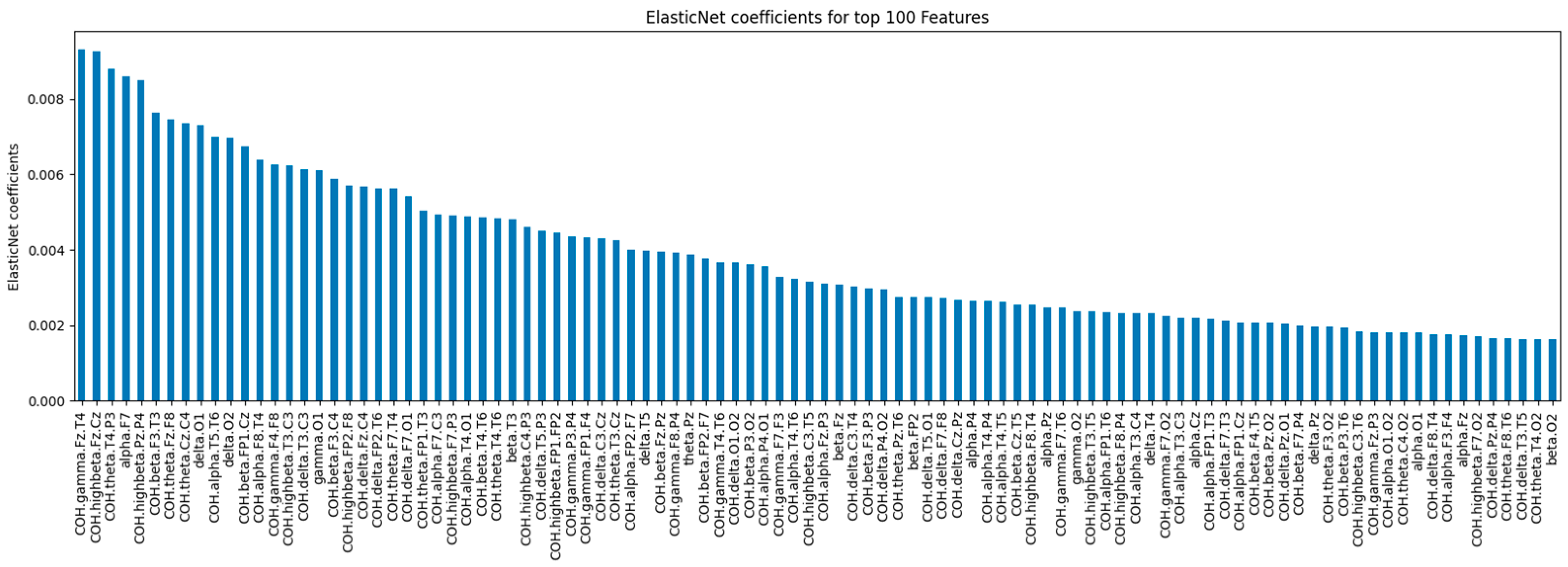
The ElasticNet model (α = 0.1, l1_ratio = 0.5) ranks feature importance by coefficient magnitude. Figure 3 shows the top 100 features by absolute coefficient values. Features on the left have larger coefficients, indicating stronger contributions to the model’s predictions, while those on the right contribute less.

3.2.2. Mutual Information-Based Feature Selection

Mutual information (MI), also known as transinformation, measures the reduction in uncertainty about one random variable (X) when given knowledge of another random variable (Y) [34]. It is a non-negative value that indicates the strength of the dependency between X and Y. Higher MI values mean stronger dependency. In other words, knowing one variable provides more information about the other if their MI value is higher. MI is a filter-based method.

MI is particularly useful for univariate feature selection, a method for identifying the most important features in a dataset. By calculating the MI between each feature and the target variable, it is possible to select the features that provide the most information about the target variable and potentially enhance the performance of machine learning models. Mutual information-based feature selection can capture any kind of statistical dependency, including linear, non-linear, and even monotonic relationships.

The mutual_info_classif function from scikit-learn was utilized to apply MI. This function relies on nonparametric methods based on entropy estimation from k-nearest neighbor distances as described by [35].

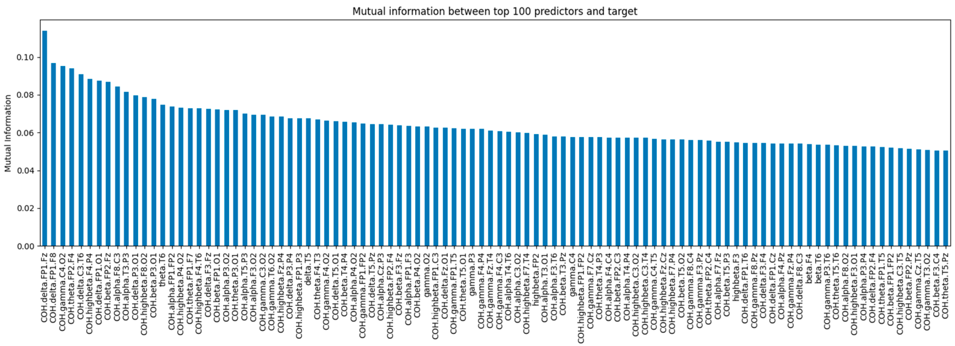
Figure 4 shows the mutual information values for the top 100 EEG-based features with the highest mutual information scores relative to the target variable (depressive disorder). These features are ranked by their MI values, indicating a strong relationship with the target variable.

3.2.3. Chi-Square-Based Feature Selection

The chi-square test assesses the dependence between stochastic variables [36]. This function helps identify and exclude features that are more likely to be independent of the class, thereby making them irrelevant for classification [37]. The following formula calculates the chi-square statistic:

$$X^2={\displaystyle \sum }_i{\displaystyle \frac{{\left(Observe{d}_i-Expecte{d}_i\right)}^2}{Expecte{d}_i}}$$

where:

• $X^2$ represents the chi-square statistic, which is a measure of how much the observed values deviate from the expected values.
• $Observe{d}_i$ is the observed or actual values.
• $Expecte{d}_i$ is the expected value if the two categories are independent.

If the categories are independent, the observed and expected values will be close. However, if there is a relationship between them, the chi-squared value will be high, indicating that the variables are likely not independent.

In this study, SelectKBest was used with the chi-squared function for feature selection, allowing independent ranking of features based on their relationship to the output variable. The sklearn.feature_selection.chi2(X, y) function calculates the chi-squared statistic for each feature, identifying those with the highest statistical significance in re-lation to the target class. This function works with non-negative features, such as Booleans or frequencies, and helps ensure that only relevant features are retained.

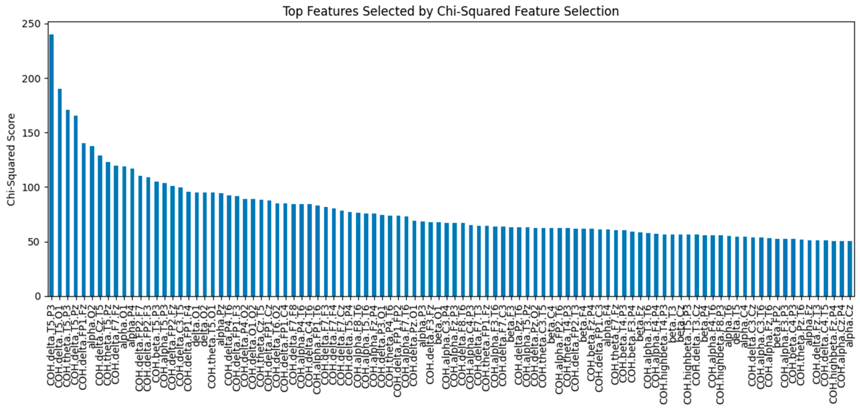
Figure 5 illustrates the chi-square statistics of the top 100 features selected using the chi-square feature selection technique. Features with higher chi-square values have a stronger relationship with the target variable.

3.2.4. Forward Feature Selection Using Stochastic Gradient Descent

Forward Feature Selection (FFS) is a wrapper method for feature selection. FFS is a greedy algorithm for selecting relevant features in machine learning models [38]. It starts with an empty model and iteratively adds features that improve the model’s performance the most. This process continues until a desired number of features is reached or a stopping criterion is met. The effectiveness of FFS is contingent upon the classifier used; thus, the choice of classifier can significantly influence the selected features and the overall model performance.

Stochastic Gradient Descent (SGD) is a popular optimization algorithm used to train various machine learning models, including those with FFS. It iteratively updates the model parameters by taking small steps in the direction of the gradient of the loss function. This allows SGD to efficiently optimize models with a large number of features [39,40].

The FFS was implemented using SGDClassifier from scikit-learn. The code iteratively selects features and trains the SGDClassifier for each feature set. The feature selection is based on maximizing the F1 score on the cross-validation set. For each iteration, a new feature is added to the feature set based on the F1 score improvement.

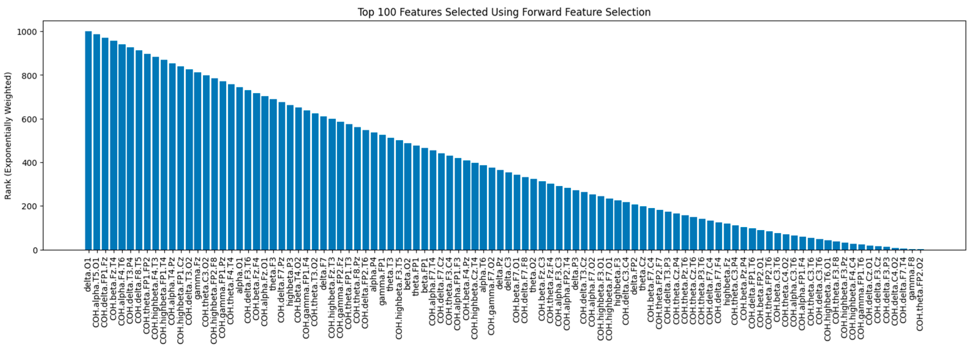
Figure 6 shows the rankings of the top 100 features selected by FFS with the SGD algorithm. Features on the left were selected earlier, indicating a stronger positive effect on the model’s performance.

3.2.5. Support Vector Machine-Based Recursive Feature Elimination

Recursive Feature Elimination (RFE) is a wrapper-based feature selection method that requires an existing classifier to guide its selection process [41]. In this case, the SVM served as the underlying model, assessing the importance of each feature based on its contribution to the SVM’s performance. This evaluation fueled RFE’s iterative removal of non-discriminative features, ultimately leading to a curated set of features ideal for SVM classification [42].

This approach, known as SVM-RFE, is a backward selection algorithm based on the SVM principle. Leveraging the strengths of SVMs in identifying informative features, it iteratively refines the feature space to retain only those that contribute most significantly to model performance. Initially, an SVM is trained on the entire training set. The coefficients of the trained SVM, which represent the relative importance of each feature in defining the decision boundary, are then analyzed. The features with the smallest absolute coefficient magnitudes are removed from the dataset. This process continues iteratively, retraining the SVM on the reduced feature set and pruning features based on their updated coefficients until the desired number of features remains. By progressively focusing on features that maximize the margin between classes, SVM-RFE efficiently improves the model’s generalizability and reduces overfitting [43]. The SVM-RFE was implemented using RFE from Scikit-learn.

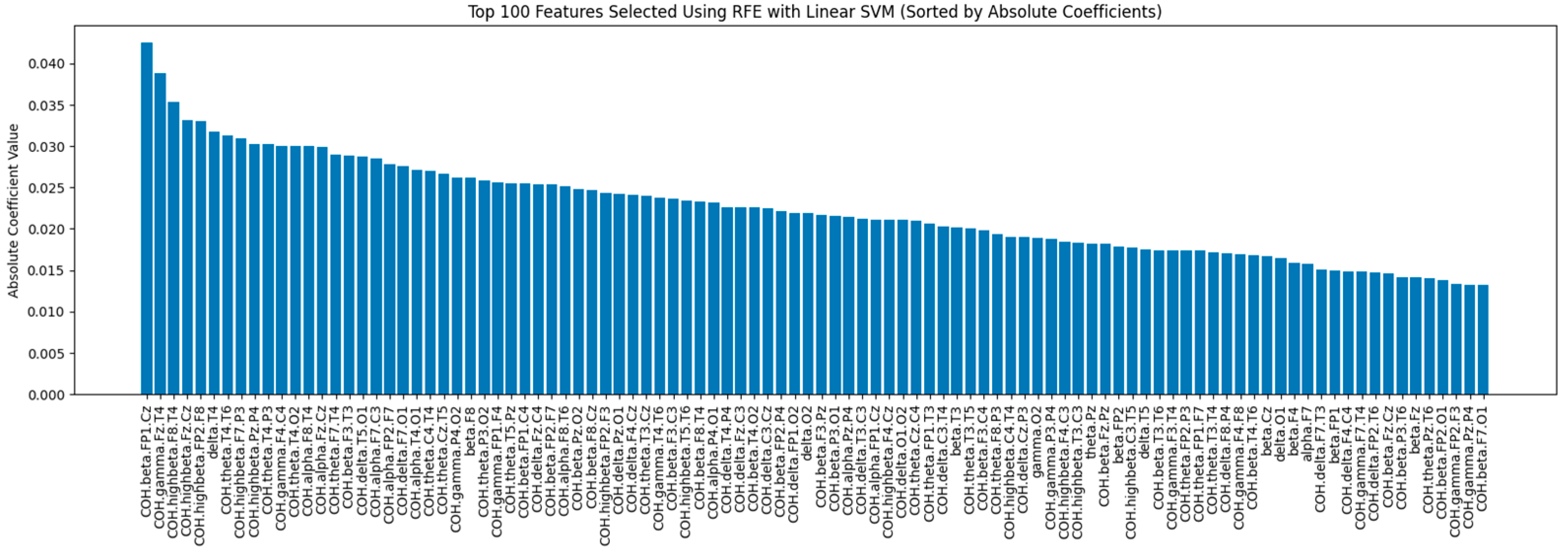
Figure 7 illustrates the absolute coefficient values of the top 100 features selected using SVM-RFE. Features with larger coefficients indicate greater importance in defining the model’s decision boundary.

3.2.6. Minimal-Redundancy-Maximal-Relevance

Minimal-redundancy-maximal-relevance (mRMR) is a filter-based feature selection method that aims to prioritize features that exhibit a high correlation with the target variable (relevance) while simultaneously minimizing redundancy among selected features. This ensures that the selected features provide unique information, enhancing the model’s ability to discriminate between different classes [44]. For continuous features, relevance is typically calculated using the F-statistic, which assesses the variance between groups, while redundancy is measured using the Pearson correlation coefficient, quantifying the linear relationship between pairs of features. This dual focus allows mRMR to effectively evaluate the importance of features in relation to both the target variable and each other [45]. Two common objective functions are Mutual Information Difference (MID) and Mutual Information Quotient (MIQ), representing the difference and quotient of relevance and redundancy, respectively [46].

In this work, mRMR was implemented using mrmr-selection 0.2.8 from Python Package Index (PyPI).

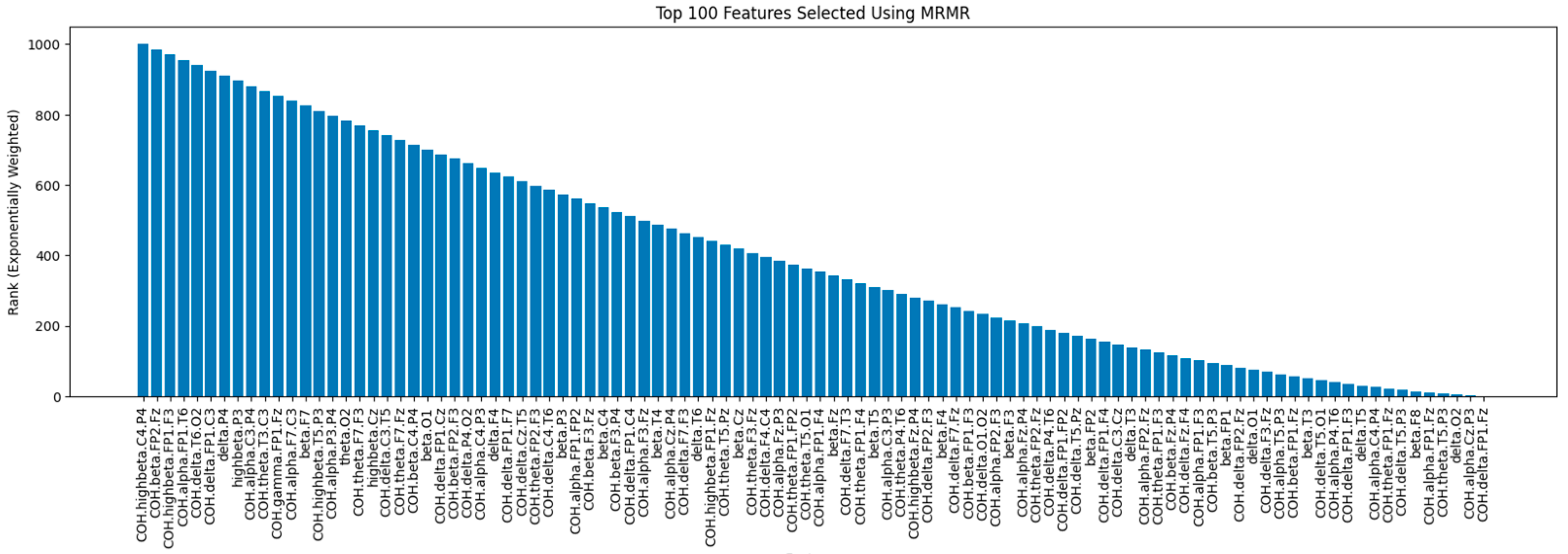
Figure 8 shows the rankings of the top 100 features selected by the mRMR method, where features are ranked based on their relevance to the target variable and their redundancy with respect to other selected features. Features on the left have higher ranks, indicating greater importance. The mRMR method ensures that the selected features provide complementary and unique information by balancing relevance and redundancy.

3.3. Models

In this study, a diverse set of classifiers was employed to ensure comprehensive coverage and robust performance across varying aspects of our binary classification task. These models include Logistic Regression, the SVM, Random Forest, and three gradient-boosting algorithms: XGBoost, CatBoost, and LightGBM. These classifiers were chosen for their ability to handle different data characteristics and complexities [47].

The six different classifiers were compared across the six selected feature sets described above. To ensure optimal performance, GridSearchCV with five-fold cross-validation was employed for hyperparameter tuning. This process systematically explored a grid of potential parameter combinations, selecting the one that yielded the best performance. In addition, given the class imbalance in the dataset, Synthetic Minority Over-sampling Technique (SMOTE) was applied to generate synthetic samples for the minority class. This step aimed to improve class balance and prevent model bias towards the majority class. The SMOTE process involved creating synthetic data points based on the k-nearest neighbors of minority class samples, thus expanding the feature space and improving the model’s ability to learn from underrepresented cases [48]. This careful approach of balancing the data and fine-tuning model parameters resulted in more reliable and accurate outcomes.

A brief description of each model along with its hyperparameters is as follows:

3.3.1. Logistic Regression

Logistic Regression is a linear model that predicts the probability of an instance belonging to a particular class by fitting a logistic curve to the data. It assumes linear relationships between features and the target variable, making it a well-established algorithm for binary classification. As a baseline model, Logistic Regression is valued for its simplicity and interpretability, with its coefficients providing insight into feature contributions to the predictions [49].

In this study, the three penalties have been evaluated {l1, l2, elasticnet}. The best performance was achieved at l2.

3.3.2. Support Vector Machine

The SVM is chosen for its effectiveness in handling high-dimensional spaces, particularly when classes are not linearly separable. The SVM works by finding the optimal hyperplane that separates classes in the feature space, maximizing the margin between them [50].

Its kernel parameter allows the selection of different types of kernels for calculating similarities between data points, such as ‘linear’, ‘poly’, ‘rbf’, or ‘sigmoid’. In this study, the ‘linear’ kernel achieved the best performance.

3.3.3. Random Forest

Random Forest is an ensemble learning method that builds multiple decision trees using random subsets of data and features. It reduces overfitting by averaging the predictions of these trees, which smooths out noise and variance, resulting in more stable and reliable outcomes [51]. Its randomness improves generalizability and robustness, making it suitable for handling complex interactions within the data.

For this study, the optimal Random Forest model was achieved with 200 decision trees (n_estimators), each limited to a depth of 10 (max_depth), and a minimum of 5 samples required before further splitting (min_samples_split).

3.3.4. XGBoost

XGBoost is a high-performance implementation of gradient boosting designed for speed and efficiency. It enhances predictive accuracy and adapts well to intricate patterns in large datasets. XGBoost works by sequentially building a series of weak learners, specifically decision trees, where each tree learns from the errors of the previous models. This iterative process makes it particularly effective for capturing complex relationships in binary classification tasks [52].

In the XGB classifier, the parameter objective = ‘binary:logistic’ specifies the objective function for binary classification tasks. The classifier parameters were optimized for the following values: learning_rate = 0.3 determines the step size shrinkage during each boosting iteration. The max_depth = 3 sets the maximum depth of each tree, controlling its complexity and helping prevent overfitting. The n_estimators = 1000 denotes the number of boosting rounds or trees in the ensemble. The subsample = 0.5 parameter controls the fraction of training data used for each boosting iteration, introducing randomness and aiding in model generalization.

3.3.5. CatBoost

CatBoost is known for its proficiency in handling categorical features, making it particularly effective in scenarios where such features are prevalent. It uses decision trees for tasks like regression, classification, and ranking, ensuring optimal performance in datasets with a mix of numerical and categorical variables. CatBoost’s unique algorithms allow it to automatically process categorical variables without extensive preprocessing, which is a significant advantage over other gradient boosting methods [53].

The CatBoost Classifier was optimized with specific parameter values to enhance its performance. The border_count = 64 determines the number of splits for numerical features. The depth = 6 parameter controls the maximum depth of each tree. The iterations = 200 indicates the number of boosting rounds or trees in the ensemble. The l2_leaf_reg = 3 introduces L2 regularization on leaf values, preventing overfitting. The learning_rate = 0.1 specifies the step size shrinkage during training, affecting the contribution of each tree to the overall model.

3.3.6. LightGBM

LightGBM is an open-source implementation of the Gradient Boosting Decision Tree (GBDT) algorithm. GBDT, a supervised learning method, aims to predict a target variable accurately by aggregating estimates from a collection of simpler and weaker models [54].

For this study, LightGBM was optimized with the following values: max_depth = 7 limits the complexity of individual trees. n_estimators = 1000 builds 1000 decision trees. num_leaves = 10 restricts each tree to a maximum of 10 leaves. subsample = 0.5 randomly uses only half of the available data for each tree, reducing variance and preventing overfitting.

3.4. Evaluation Metrics

The evaluation metrics employed in this study are accuracy, precision, recall (sensitivity), the F1 score, and ROC curves. These metrics offer critical insight into the performance of the machine learning models applied to the depression detection task using EEG data. The metrics are computed for each model using 5-fold cross-validation, with the StratifiedKFold method ensuring that the class distribution was preserved across different subsets of data for consistent and reliable evaluation [55].

The model training process involved splitting the dataset into five equal-sized folds. In each iteration, one fold was used as the validation set while the other four folds were used for training, ensuring that each data point was used for both training and validation exactly once. This process was repeated five times, with the final performance metrics averaged across all iterations to provide a robust estimate of model performance. This cross-validation approach helped reduce the risk of overfitting and ensured a more generalized assessment across different subsets of the data.

Preprocessing steps included normalizing the EEG data to standardize feature values. For each training fold, feature selection methods (e.g., SVM-RFE, Elastic Net) were applied to avoid data leakage. The selected feature set was then used for training the classifiers, whose hyperparameters were optimized using GridSearchCV, as outlined in Section 3.3.

• Accuracy is the percentage of correctly classified data points (both true positives and true negatives) out of the total number of instances [56]:

  $$Accuracy={\displaystyle \frac{\mathrm{TP}+\mathrm{TN}}{\mathrm{TP}+\mathrm{TN}+\mathrm{FP}+\mathrm{FN}}}$$

  where TP = True Positives, TN = True Negatives, FP = False Positives, FN = False Negatives.
• Precision measures the accuracy of positive predictions by evaluating the percentage of correct positive predictions relative to all predicted positives. It is calculated as the ratio of true positives to the sum of true positives and false positives:

  $$Precision={\displaystyle \frac{\mathrm{TP}}{\mathrm{TP}+\mathrm{FP}}}$$
• Recall, also known as sensitivity or true positive rate, measures the proportion of actual positive instances that were correctly predicted by the model. It represents the percentage of actual positive data points that are correctly predicted:

  $$Recall={\displaystyle \frac{\mathrm{TP}}{\mathrm{TP}+\mathrm{FN}}}$$
• F1 score is the harmonic mean of precision and recall, providing a balanced measure of model performance. The F1 score is defined as:

  $$F1={\displaystyle \frac{2·\mathrm{Precision}·\mathrm{Recall}}{\mathrm{Precision}+\mathrm{Recall}}}$$
• ROC curves plot the true positive rate against the false positive rate by adjusting the classifier’s threshold or score for class membership. The area under the ROC curve (AUC) is a single metric that is used for assessing and comparing classifier performance. It represents the probability that a classifier will rank a randomly chosen positive instance higher than a randomly chosen negative instance. AUC values range from 0 to 1, with a higher value indicating better performance across all possible thresholds. ROC curves are widely used to visually compare the performance of binary classifiers.

These metrics are particularly useful in binary classification tasks, where the goal is to differentiate between two classes (e.g., depression vs. non-depression). They provide a comprehensive assessment of model performance, considering both correct and incorrect predictions and highlighting trade-offs between precision and recall [56].

4. Results

The performance of six different machine learning models was evaluated using both feature selection methods and without feature selection for the depression detection task using EEG data. The results were analyzed using the key metrics discussed earlier: accuracy, precision, recall, and F1 score.

Table 2. Performance metrics of machine learning models with various feature selection methods.

Feature Selection	Algorithm Name	Accuracy (%)	Precision (%)	Recall (%)	F1 Score (%)
Support Vector Machine-based Recursive Feature Elimination	SVM	93.54	94.68	95.97	95.29
	Logistic Regression	92.86	93.46	96.46	94.84
	XGBoost	77.55	80.99	87.44	84.07
	LGBM	75.18	80.01	84.94	82.3
	Random Forest	75.17	78.56	87.42	82.67
	CatBoost	74.15	77.89	86.41	81.89
Elastic Net	SVM	90.47	92.91	93.44	93.01
	Logistic Regression	90.47	92.71	93.44	93.0
	Random Forest	77.87	80.19	89.4	84.43
	XGBoost	77.56	82.85	84.44	83.57
	CatBoost	76.2	80.63	85.44	82.94
	LGBM	75.51	80.13	84.92	82.45
Mutual Information	Random Forest	77.53	82.08	85.37	83.62
	LGBM	76.19	81.33	84.4	82.69
	CatBoost	75.16	79.45	85.4	82.21
	XGBoost	74.49	80.33	82.9	81.47
	Logistic Regression	66.99	76.83	73.31	74.81
	SVM	65.63	75.75	72.29	73.67
Minimal-Redundancy-Maximal-Relevance	Random Forest	76.17	80.55	85.4	82.86
	LGBM	73.13	79.33	81.92	80.46
	CatBoost	73.12	79.83	80.88	80.21
	XGBoost	71.42	79.63	78.37	78.75
	SVM	66.32	76.56	72.86	74.58
	Logistic Regression	65.98	77.78	70.35	73.7
Chi-Square	Random Forest	75.51	79.64	85.9	82.53
	CatBoost	73.12	80.1	80.36	80.04
	LGBM	72.43	79.51	79.87	79.54
	XGBoost	67.34	77.39	72.85	74.93
	Logistic Regression	64.63	76.58	70.33	72.85
	SVM	63.94	74.6	71.33	72.69
Forward Feature Selection with Stochastic Gradient Descent	Random Forest	73.48	78.44	83.94	81.03
	XGBoost	71.78	79.05	79.41	79.18
	CatBoost	71.43	77.25	81.91	79.42
	LGBM	71.43	77.63	81.4	79.35
	SVM	66.67	77.05	72.36	74.59
	Logistic Regression	66.0	76.55	71.87	74.11
Without Feature Selection	CatBoost	70.72	77.21	80.37	78.57
	XGBoost	69.71	76.83	78.85	77.23
	Random Forest	68.34	73.73	82.91	77.99
	LGBM	67.32	74.24	78.36	75.91
	SVM	66.31	75.74	75.33	74.59
	Logistic Regression	64.27	75.72	71.32	72.27

, which is sorted by model performance, presents a detailed summary of these metrics for each model across various feature selection techniques, providing a clear view of how the selection method impacts performance.

The SVM-RFE method produced the best overall performance, particularly for the SVM and Logistic Regression. The SVM achieved an accuracy of 93.54%, with very high precision (94.68%) and recall (95.97%), resulting in an F1 score of 95.29%. Logistic Regression also performed well, achieving 92.86% accuracy. The success of RFE for these models is due to its iterative nature, where it removes the least important features and retrains the model on the remaining features. This method is especially effective for linear models when the feature space is high-dimensional, such as EEG data, because it eliminates redundant or irrelevant features while preserving the key signals that are most important. However, tree-based models like Random Forest and XGBoost performed significantly lower than the linear models. This reduced performance could be due to RFE’s feature-removal process, which may disrupt the internal structure of tree-based models. These models are inherently designed to handle feature redundancy and importance internally, relying more on complex feature interactions than strict feature elimination, which explains their lesser dependence on external feature selection methods [57].

With Elastic Net as the feature selection method, both the SVM and Logistic Regression achieved the highest accuracy (90.47%), with almost identical precision and recall values, resulting in very high F1 scores (93.00%). This indicates that Elastic Net is particularly effective for linear models, as it balances feature selection and regularization properties, which prevents overfitting and ensures the models focus on the most relevant features, particularly in high-dimensional EEG data. Tree-based models like Random Forest and XGBoost saw a performance boost compared to their results without feature selection, with Random Forest reaching 77.87% accuracy and XGBoost achieving 77.56%. However, their low performance compared to the linear ones indicates that tree-based models may have lost some key features during the Elastic Net regularization process.

With mutual information, non-linear models like Random Forest (77.53% accuracy) and LGBM (76.18% accuracy) performed better than linear models such as the SVM (65.63%) and Logistic Regression (66.99%). This is because mutual information captures non-linear relationships between features, which non-linear models can take advantage of. In contrast, linear models struggle to use these complex interactions, leading to lower performance. Non-linear models handle these relationships more effectively, giving them an advantage in this case.

mRMR also favored non-linear models, with Random Forest achieving the highest accuracy (76.17%) and F1 score (82.86%). LGBM and XGBoost also performed well with mRMR, showing that non-linear models can leverage complementary features to build stronger predictive power. However, linear models like the SVM and Logistic Regression struggled with this method, as they rely more on direct feature relevance rather than interactions between features.

The chi-squared feature selection approach yielded the best results for Random Forest, which achieved 75.51% accuracy, with a high F1 score of 82.53%. Tree-based models, such as CatBoost and LGBM, also performed reasonably well. However, the SVM and Logistic Regression once again struggled with lower accuracy rates (63.93% and 64.63%, respectively), highlighting the limitations of chi-squared when applied to linear models.

Forward Feature Selection using SGD performed similarly for tree-based models like CatBoost, Random Forest, and XGBoost, with accuracy scores hovering between 71.43% and 73.48%. However, linear models like the SVM and Logistic Regression underperformed, achieving accuracy scores of 66%. This indicates that forward selection, which adds features incrementally, may not work as well for linear models when the feature space is complex, as it cannot exploit complex feature interactions that non-linear models can.

Without feature selection, CatBoost achieved the highest accuracy (70.72%), followed closely by XGBoost (69.71%) and Random Forest (68.34%). However, these models struggled with precision and recall, indicating that the models were not adequately capturing the complex patterns in the data. The SVM and Logistic Regression performed worst, likely because these linear models are more sensitive to irrelevant or redundant features in high-dimensional data, such as EEG signals, where selecting key features can be critical to performance.

Across the various feature selection methods, the combination of SVM-RFE with the SVM emerged as the top performer, with the SVM achieving the highest accuracy of 93.54% and Logistic Regression following closely at 92.86%. Elastic Net also proved to be a powerful feature selection technique for the SVM and Logistic Regression, with both models performing exceptionally well. On the other hand, tree-based models like Random Forest, XGBoost, and CatBoost performed better with mutual information, chi-squared, and mRMR feature selection methods, indicating that these techniques better capture the complex, non-linear relationships in the data.

Figure 9 illustrates the trends across feature selection methods visually. As shown, SVM-RFE and Elastic Net allow linear models like Logistic Regression and the SVM to outperform non-linear models.

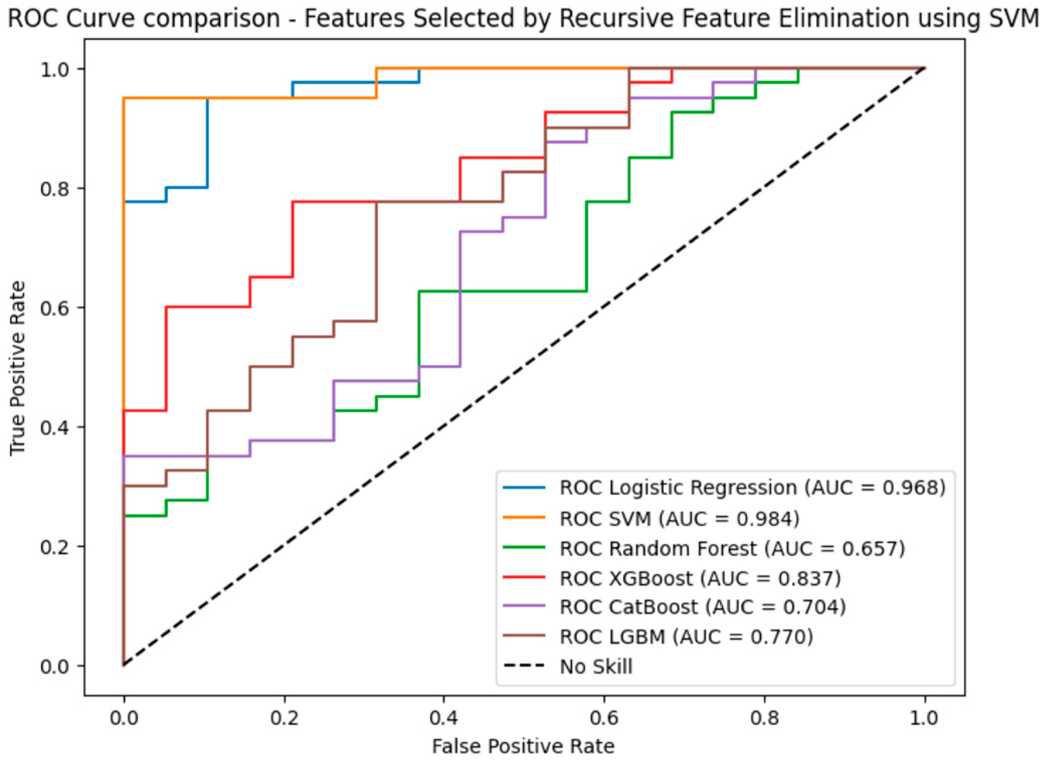
Since the results demonstrate that features selected using SVM-RFE resulted in the best performance based on accuracy, precision, recall, and F1 score, ROC curves were used to further evaluate the performance. In this evaluation, the SVM achieved the highest AUC (0.984), followed by Logistic Regression (AUC = 0.968), indicating strong classification performance. XGBoost performed moderately with an AUC of 0.837, while tree-based models like LGBM (AUC = 0.770) and CatBoost (AUC = 0.704) showed more modest results. Random Forest had the lowest AUC (0.657), as shown in Figure 10.

Comparison of Findings with Existing Works

The findings from our study highlight the effectiveness of SVM-RFE in handling high-dimensional EEG data for depression detection, achieving an accuracy of 93.54%. This result aligns with the broader trend in the literature emphasizing the importance of targeted feature selection in improving model accuracy. The iterative nature of RFE systematically removes irrelevant features, enhancing predictive capability, which is consistent with previous works highlighting the importance of feature selection in clinical prediction accuracy [58].

Our results demonstrate that simpler models with effective feature selection can achieve competitive performance compared to more complex methods. For example, Ref. [59] reported 94.72% accuracy using a sophisticated model incorporating spatiotemporal information and weighted feature fusion, while [60] achieved 89.02% with an ensemble approach combining Deep Forest and the SVM. Compared to both methods, our SVM-RFE approach delivered comparable or better outcomes, suggesting that RFE can bridge the gap between traditional machine learning techniques and more complex approaches.

Comparatively, ref. [61] reported that feature extraction methods such as Principal Component Analysis (PCA), combined with Logistic Regression, yielded 89.04% accuracy for depression prediction. While feature extraction can be beneficial for dimensionality reduction, our findings suggest that targeted feature selection techniques like RFE may offer a more tailored approach to handling high-dimensional data, thereby achieving higher accuracy.

When compared with other studies, our results demonstrate a competitive edge. For instance, the authors of [62] reported classification accuracies ranging from 80% to 95% across various classifiers trained on linear and non-linear EEG features. In addition, the technique described in [63] achieved 88.33% accuracy using the SVM with features such as alpha2 and theta asymmetry, applying Multi-Cluster Feature Selection (MCFS). While the study in [63] highlighted the importance of specific EEG features, our higher accuracy suggests that SVM-RFE’s iterative feature elimination process may offer a more refined approach for optimizing model performance by focusing on the most relevant features. Similarly, the method described in [64] achieved 91.07% accuracy on a training set and 84.16% on an independent test set using CK-SVM with coherence-based features selected through sequential backward selection.

Furthermore, tree-based models in this study demonstrated performance gains with certain feature selection methods (e.g., mutual information, mRMR), which aligns with the findings by the authors of [65], who highlighted the importance of using selection techniques that cater to non-linear relationships in EEG data.

Overall, the comprehensive evaluation of machine learning models and feature selection techniques in our study underscores the value of targeted selection methods like SVM-RFE for achieving strong performance in EEG-based depression detection.

5. Conclusions and Future Work

Depression detection using EEG data holds promise for improving diagnostic accuracy in mental healthcare. This study demonstrates how feature selection techniques optimize classifier performance. The utilization of features selected through the wrapper-based method SVM-RFE and the embedded-based method Elastic Net proved to yield the most optimal performance among the six classifiers evaluated. SVM-RFE for feature selection with the SVM classifier demonstrated the highest accuracy of 93.54%, followed closely by Logistic Regression with 92.86% accuracy. Elastic Net-based feature selection also provided strong results, with SVM achieving 90.47% accuracy and Logistic Regression matching it with 90.47%. This highlights the significant impact of feature selection on the performance of classifiers, even when considering hyperparameter tuning.

Implementing these findings in clinical practice could enhance the early detection and management of major depressive disorder, improving patient outcomes and quality of life. Addressing ethical considerations and practical challenges associated with applying these findings in clinical settings is essential. Furthermore, integrating multimodal data with EEG data holds the potential for creating more robust models. Also, large-scale validation studies across diverse populations and settings are crucial for generalizability.