Multi-Objective Optimization of Three-Stage Turbomachine Rotor Based on Complex Transfer Matrix Method

Abstract

This study presents the complex transfer matrix method (CTMM) as an advanced mathematical model, providing significant advantages over the finite element method (FEM) by yielding rapid solutions for complex optimization problems. In order to design a more efficient structure of a three-stage turbomachine rotor, we integrated this method with various optimization algorithms, including genetic algorithm (GA), differential evolution (DE), simulated annealing (SA), gravitational search algorithm (GSA), black hole (BH), particle swarm optimization (PSO), Harris hawk optimization (HHO), artificial bee colony (ABC), and non-metaheuristic pattern search (PS). Thus, the best rotor geometry can be obtained fast with minimum bearing forces and disk deflections within design limits. In the results, the efficiency of the CTMM for achieving optimized designs is demonstrated. The CTMM outperformed the FEM in both speed and applicability for complex rotordynamic problems. The CTMM was found to deliver results of comparable quality much faster than the FEM, especially with higher element quality. The use of the CTMM in the iterative optimization process is shown to be highly advantageous. Furthermore, it is noted that among the different optimization algorithms, ABC provided the best results for this multi-objective optimization problem.

1. Introduction

The designs of turbomachines are carried out through several stages, such as conceptual design, preliminary design, and detailed design. Throughout these design processes, multiple iterations and optimization studies are conducted to enhance system performance and increase reliability and efficiency. Examples of such iterations include disk topology optimization [1], diffuser performance optimization for axial turbines [2], optimization of single-stage radial-outflow turbines [3], and performance evaluation of turbines [4]. Identifying issues such as dynamic behavior, vibration levels, critical speeds, and mechanical fatigue early on prevents major changes during testing and analysis. This helps avoid unnecessary costs and mitigates critical design risks. One of the most crucial components determining this dynamic behavior in a turbomachine is the rotor, as rotordynamics play a crucial role in rotating machinery design [5]. 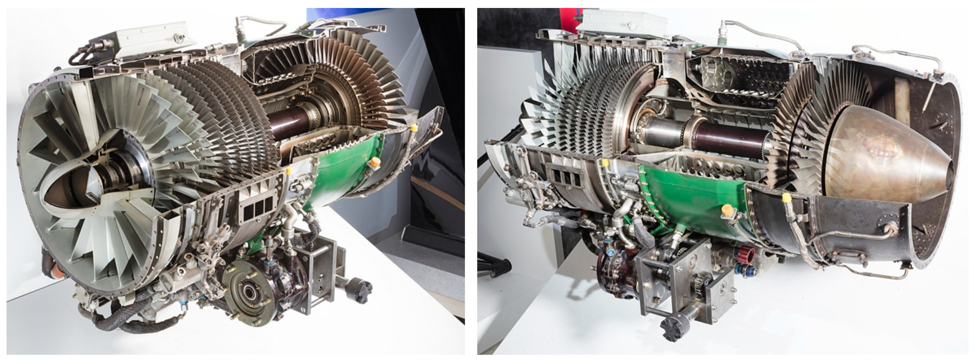The design of rotors for turbomachines, as shown in Figure 1, presents a significant engineering challenge due to their high rotational speeds. This complexity is further complicated by numerous variables and multiple objectives that need to be met in extreme conditions, such as high altitudes, elevated temperatures, and rapid changes in operational dynamics. Under these circumstances, the rotor must operate without inducing excessive bearing loads, while maintaining safe vibration levels and avoiding contact with stationary components at high speeds. To meet these multifaceted requirements and address nonlinear relationships, rotordynamic optimization is essential.

Rotordynamic optimization spans various distinct areas, such as adjustable bearing optimization [6], hydrodynamic journal bearing optimization [7], dynamic optimization for non-continuous rotors [8], swirl brake optimization for rotordynamic performance [9], and stability analysis of rotor-bearing systems under the influence of misalignment [10]. These efforts reflect the multifaceted requirements of rotordynamics that are essential for achieving optimal system performance. When examining these optimization studies, it becomes clear that different optimization algorithms are employed, depending on the objectives because optimization algorithms can exhibit varying performance based on the specific problem type. Examples include genetic algorithm (GA) for design optimization [11], differential evolution (DE) for reducing vibration levels [12], simulated annealing (SA) for multi-objective optimization [13], particle swarm optimization (PSO) for modeling twin rotor systems [14], and Harris hawk optimization (HHO) for addressing unbalance characteristics [15]. Each of these methods presents distinct advantages depending on the complexity of the rotordynamic problem being tackled. A shared characteristic of these studies is their reliance on the finite element method (FEM). Key results, such as natural frequencies, stability, and bearing forces—set as objective functions—are typically derived through FEM-based black-box solvers, either developed by researchers or accessed via commercial software. However, the FEM can be computationally intensive, and in certain cases, alternative mathematical models may offer more efficient and faster solutions.

An alternative mathematical model to the FEM is the transfer matrix method (TMM), which is widely used in diverse intricate system such as rotor-bearing systems [16,17], multibody systems [18], acoustic systems [19], and optical systems [20]. The advantage of fast solutions makes this method suitable for optimization and has led to its application across a diverse range of areas [21,22,23]. Despite these benefits, there is currently no study highlighting the TMM’s superiority over the FEM in structural applications or exploring its advantages in optimization. The TMM delivers results that closely align with analytical methods and provides high-quality, efficient solutions regardless of the number of elements. Given this capability, it follows that the TMM will offer significant advantages in optimization studies, provided that a mathematical model of a system is established. To address this gap, we applied the complex transfer matrix method (CTMM) for rotordynamic optimization with modern metaheuristic optimization algorithms.

Figure 1. General Electric J85-GE [24]. Image courtesy of Smithsonian’s National Air and Space Museum.

Figure 1. General Electric J85-GE [24]. Image courtesy of Smithsonian’s National Air and Space Museum.

To comprehensively evaluate the optimization performance of the CTMM, a variety of algorithms was selected to cover a broad range of techniques and development periods. These algorithms are categorized based on their underlying principles, such as evolution-based, swarm-based, and physics-based approaches. The selection spans from early metaheuristic techniques like GA to modern algorithms such as HHO. The integration of these algorithms with the CTMM for structural analysis optimization represents a novel approach not previously documented in the literature. Consequently, to emphasize the CTMM’s superiority over the FEM, a wide array of optimization algorithms was employed in conjunction with the CTMM.

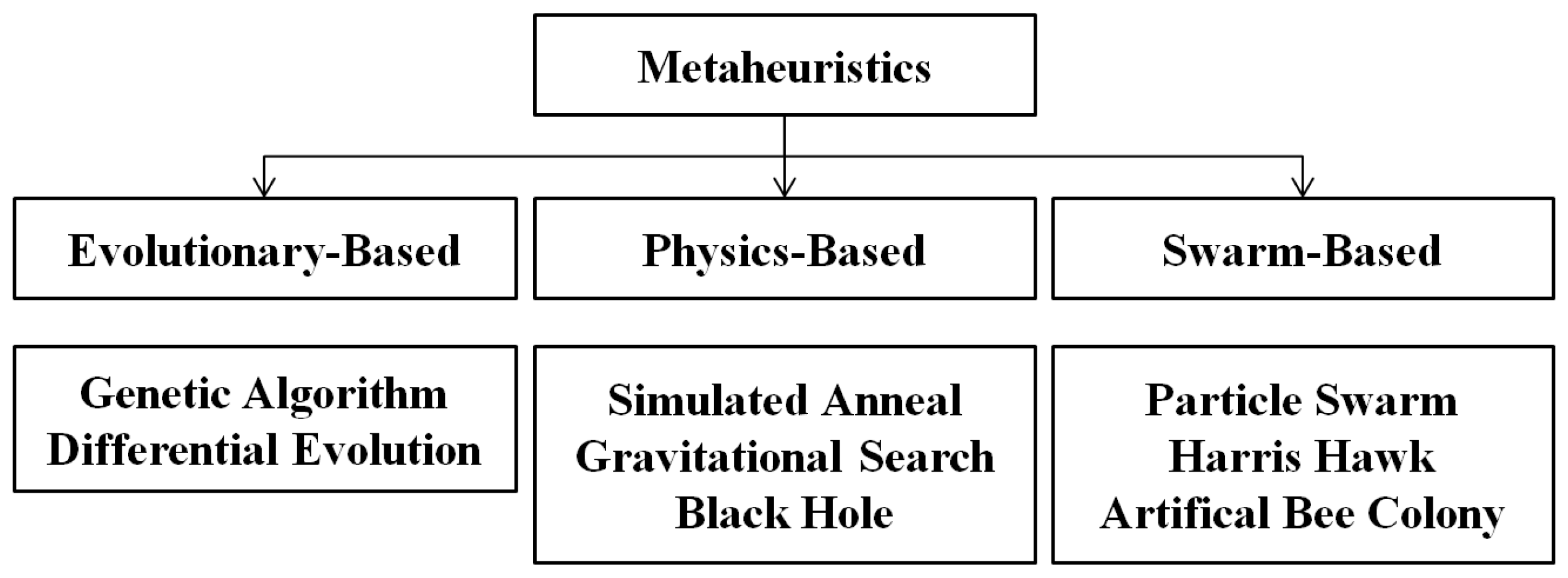
Our objective was to ensure a diverse selection of algorithms while limiting the number to avoid complicating the evaluation process. Thus, we extend the evaluation of optimization algorithms by including not only metaheuristic methods but also the pattern search (PS) algorithm. This results in a total of nine different optimization algorithms considered for rotordynamic optimization. These algorithms encompass evolutionary-based approaches (GA and DE), physics-based methods (SA, GSA, and black hole (BH)), and swarm-based techniques (PSO, HHO, and artificial bee colony (ABC)). Sharing the common feature of being gradient-free, these algorithms were used to optimize the rotordynamics of a multimodal and multivariable three-stage turbomachine using the CTMM and their performances were evaluated.

2. Transfer Matrix Theory

In the early twentieth century, computational technology was still in its early stages, which required engineers to rely on various manual calculation methods and early computers with array-based systems. To address this challenge, the TMM was first introduced by Holzer [25] and Myklestad [26]. The TMM is a computational method that uses matrices to transfer the relationships between the defined degrees of freedom and generalized forces within a system. The system characteristics are obtained by multiplying these matrices in the order of their physical configuration. Today, with its expression in the complex plane, the TMM is utilized to analyze the dynamic behavior of complex systems in both steady-state and transient conditions [27].

2.1. Transfer Matrix Method

The TMM shares similarities with methods used in analyzing robotic systems or graphical techniques, where the positional information of a point is transformed using matrices and transferred to another point. Beyond position, the TMM also facilitates the transfer of physical quantities such as force and moment. This is achieved through the use of transfer matrices that operate across state vectors.

In the implemented rotordynamic solver, axial and torsional motions were excluded to concentrate on bending motion, which is more critical for turbofan engine rotors [28]. To account for the effect of critical speed, gyroscopic effects were incorporated into the model, with bending motion defined along two lateral axes. The Timoshenko beam theory was applied in the rotordynamic solver, using state vectors with nine parameters, as presented in Equation (1). The rotor analyzed belongs to the LP (low-pressure) rotor group and is therefore exposed to considerably lower temperatures than the HP (high-pressure) rotor group. This design feature concentrates the primary thermal effects on the turbine section, while the shaft remains relatively cooler, a favorable condition in turbomachinery design. Consequently, the rotor’s stiffness and natural frequency experience only minimal reductions due to thermal expansion [29,30], making it reasonable to assume that thermal effects may be omitted in the preliminary optimization phase.

As detailed in Equation (1), X and Y denote lateral vibration freedoms, as illustrated in Figure 2. ${\theta }_y$ represents shear rotation around the X-axis, while ${\theta }_x$ represents shear rotation around the Y-axis. $M_y$ and $M_x$ denote shear moments, and $V_x$ and $V_y$ represent shear forces. External loads are introduced via the final unit parameter.

$$\left\{Z_i\right\}={ \left[X {\theta }_y M_y-V_x-Y {\theta }_x M_x V_y 1 \right]}^T$$

(1)

The coordinate system used in the CTMM is shown in Figure 2. In the solver created, the Z-axis represents the rotational axis, the X-axis defines the direction of the side, and the Y-axis represents the vertical direction. The leftmost point of the rotor corresponds to the (0, 0, 0) point in this coordinate system.

In this state vector, the system response at the ith node is multiplied by the transfer matrix of the ith element to compute the system response at the (i + 1)th node, as described in Equation (2).

$$\left\{Z_{i+1}\right\}=\left[U_i\right]\left\{Z_i\right\}$$

(2)

To initiate the process, transfer matrix elements must be developed to accurately represent the characteristics of the desired unit system. Once these element matrices are defined appropriately, they are sequentially multiplied in the order that suits the design configuration to derive the system’s transfer matrix. Using this transfer matrix, both the steady-state system response and the examination of mode shapes and natural frequencies can be conducted.

2.2. Element Matrices

In rotordynamics, the TMM comprises four fundamental elements. Shown in Figure 3 from left to right are the bearing element matrix, disk element matrix, beam element matrix, and unbalance element matrix. These matrices are defined within the coordinate system depicted in Figure 2.

2.2.1. Bearing Element Matrix

The element used to secure the rotor structure to the stationary part is referred to as the bearing element matrix. Linear stiffness and linear damping expressions are utilized in this matrix, as shown in Equation (3). While Equation (3) defines the matrix for a single axis, X or Y, its generalized form is provided in Equation (4).

$${\left[U_{BEARIN{G}_{X,Y}}\right]}_{4\times 4}={\left[\begin{array}{cccc} 1& 0 & 0 & 0 \\ 0& 1 & 0 & 0 \\ 0& 0 & 1 & 0 \\ -\left(K+j\omega C\right)& 0 & 0 & 1 \end{array}\right]}_{4\times 4}$$

(3)

$${\left[U_{BEARING}\right]}_{8\times 8}={\left[\begin{array}{cc} {\left[U_{BEARIN{G}_X}\right]}_{4\times 4}& O_{4\times 4} \\ O_{4\times 4}& {\left[U_{BEARIN{G}_Y}\right]}_{4\times 4} \end{array}\right]}_{8\times 8}$$

(4)

2.2.2. Disk Element Matrix

The disks on the rotor are modeled as point masses with specified inertia and mass values. This inertia characteristic influences the natural frequency of the rotor under gyroscopic effects. Similar to the bearing element matrix, this inertia is defined separately for the X- and Y-axes as shown in Equations (5) and (6), and the combined expression is given in Equation (7).

$${\left[U_{POIN{T}_X}\right]}_{4\times 4}={\left[\begin{array}{cccc} 1& 0& 0& 0 \\ 0& 1& 0& 0 \\ 0& { I}_p\Omega \omega -I_d{\omega }^2& 1& 0 \\ M{\omega }^2& 0& 0& 1 \end{array}\right]}_{4\times 4}$$

(5)

$${\left[U_{POIN{T}_Y}\right]}_{4\times 4}={\left[\begin{array}{cccc} 1& 0& 0& 0 \\ 0& 1& 0& 0 \\ 0& -I_p\Omega \omega -I_d{\omega }^2& 1& 0 \\ M{\omega }^2& 0& 0& 1 \end{array}\right]}_{4\times 4}$$

(6)

$${\left[U_{POINT}\right]}_{8\times 8}={\left[\begin{array}{cc} {\left[U_{POIN{T}_X}\right]}_{4\times 4}& O_{4\times 4} \\ O_{4\times 4}& {\left[U_{POIN{T}_Y}\right]}_{4\times 4} \end{array}\right]}_{8\times 8}$$

(7)

2.2.3. Beam Element Matrix

The matrix defining the shaft properties is known as the field element matrix. Coefficients in this matrix are derived using the Krylov equation, in accordance with the Timoshenko beam theory [31], as shown in Equation (8).

$${\displaystyle \frac{{\delta }^{4}Y\left(z\right)}{\delta z^4}}+{\displaystyle \frac{\overline{m}{\omega }^2}{E{I}_d}}\left({\displaystyle \frac{E{I}_d}{G{A}_s}}+{\rho }_z^2\right)-{\displaystyle \frac{\overline{m}{\omega }^2}{E{I}_d}}\left(1-{\displaystyle \frac{\overline{m}{\rho }_z^2{\omega }^2}{G{A}_s}}\right)Y(z)=0$$

(8)

In this equation, $\overline{m}$ represents the mass per unit length, $E$ represents the elastic modulus, $G$ represents the shear modulus, ${\rho }_z$ represents the radius of gyration, and $A_s$ represents the cross-sectional area. Equation (8) can be derived and expressed in terms of the parameters of the state vector in Equation (1), as shown in the following equations.

$$Y^i\left(z\right)=A^i\mathrm{c}\mathrm{o}\mathrm{s}\mathrm{h}\left({\lambda }_{1}z\right)+B^i\mathrm{s}\mathrm{i}\mathrm{n}\mathrm{h}\left({\lambda }_{1}z\right)+C^i\mathrm{c}\mathrm{o}\mathrm{s}\left({\lambda }_{2}z\right)+D^i\mathrm{s}\mathrm{i}\mathrm{n}\left({\lambda }_{2}z\right)$$

(9)

$${\theta }^i\left(z\right)=A^i{F}_1\mathrm{s}\mathrm{i}\mathrm{n}\mathrm{h}\left({\lambda }_{1}z\right)+B^i{F}_1\mathrm{c}\mathrm{o}\mathrm{s}\mathrm{h}\left({\lambda }_{1}z\right)+C^i{F}_2\mathrm{s}\mathrm{i}\mathrm{n}\left({\lambda }_{2}z\right)-D^i{F}_2\mathrm{c}\mathrm{o}\mathrm{s}\left({\lambda }_{2}z\right)$$

(10)

$$M^i\left(z\right)=A^i{E}_1\mathrm{c}\mathrm{o}\mathrm{s}\mathrm{h}\left({\lambda }_{1}z\right)+B^i{E}_1\mathrm{s}\mathrm{i}\mathrm{n}\mathrm{h}\left({\lambda }_{1}z\right)+C^i{E}_2\mathrm{c}\mathrm{o}\mathrm{s}\left({\lambda }_{2}z\right)+D^i{E}_2\mathrm{s}\mathrm{i}\mathrm{n}\left({\lambda }_{2}z\right)$$

(11)

$$V^i\left(z\right)=A^i{\displaystyle \frac{\overline{m}{\omega }^2}{{\lambda }_1}}\mathrm{s}\mathrm{i}\mathrm{n}\mathrm{h}\left({\lambda }_{1}z\right)+B^i{\displaystyle \frac{\overline{m}{\omega }^2}{{\lambda }_1}}\mathrm{c}\mathrm{o}\mathrm{s}\mathrm{h}\left({\lambda }_{1}z\right)+C^i{\displaystyle \frac{\overline{m}{\omega }^2}{{\lambda }_2}}\mathrm{s}\mathrm{i}\mathrm{n}\left({\lambda }_{2}z\right)-D^i{\displaystyle \frac{\overline{m}{\omega }^2}{{\lambda }_2}}\mathrm{c}\mathrm{o}\mathrm{s}\left({\lambda }_{2}z\right)$$

(12)

The expansions of the abbreviations $E_1$, $E_2$, $F_1$, $F_2$, ${\lambda }_1$, and ${\lambda }_2$, used in the equations are provided in the following equations:

$$E_1=E{I}_d\left({\displaystyle \frac{\overline{m}{\omega }^2}{G{A}_s}}+{{\lambda }_1}^2\right), E_2=E{I}_d\left({\displaystyle \frac{\overline{m}{\omega }^2}{G{A}_s}}-{{\lambda }_2}^2\right)$$

(13)

$$F_1={\displaystyle \frac{\overline{m}{\omega }^2}{G{A}_s{\lambda }_1}}+{\lambda }_1, F_2={\displaystyle \frac{\overline{m}{\omega }^2}{G{A}_s{\lambda }_2}}-{\lambda }_2$$

(14)

$${\lambda }_{\mathrm{1,2}}=\sqrt{\sqrt{{\left({\displaystyle \frac{\overline{m}{\omega }^2}{E{I}_d}}\right)}^4+{\displaystyle \frac{1}{4}}{\left({\displaystyle \frac{\overline{m}{\omega }^2}{G{A}_s}}-{\displaystyle \frac{\overline{m}{\rho }_z^2{\omega }^2}{E{I}_d}}\right)}^2\pm } {\displaystyle \frac{1}{2}}{\displaystyle \frac{\overline{m}{\omega }^2}{G{A}_s}}+{\displaystyle \frac{\overline{m}{\rho }_z^2{\omega }^2}{E{I}_d}}}$$

(15)

Since the matrix coefficients obtained involve complex differential expressions that vary with shaft parameters, [${\delta }_X$] and [${\delta }_Y$] are used here to represent the generalized forms along the X- and Y-axes. The combined expression of the matrix is provided in Equation (16).

$${\left[U_{FIELD}\right]}_{8\times 8}={\left[\begin{array}{cc} {\left[{\delta }_X\right]}_{4\times 4}& O_{4\times 4} \\ O_{4\times 4}& {\left[{\delta }_Y\right]}_{4\times 4} \end{array}\right]}_{8\times 8}$$

(16)

2.2.4. Unbalance Element Matrix

It was initially assumed that the unbalance expression was confined to the XY-plane. To achieve this, the unbalance matrix was formulated as shown in Equation (17). The matrix size of 9 × 9 accommodates the addition of force expressions in the rightmost column. While this matrix expands for solutions in other matrices, it does not include powers and is defined as unit.

$${\left[U_{UNBALANCE}\right]}_{9\times 9}={\left[\begin{array}{c}{I}_{3\times 3}\\ O_{1\times 3}\\ O_{3\times 3}\\ O_{1\times 3}\\ O_{1\times 3}\end{array} \begin{array}{c}{O}_{3\times 1}\\ 1\\ O_{3\times 1}\\ 0\\ 0\end{array} \begin{array}{c}{O}_{3\times 3}\\ O_{1\times 3}\\ I_{3\times 3}\\ O_{1\times 3}\\ O_{1\times 3}\end{array} \begin{array}{c}{O}_{3\times 1}\\ 0\\ O_{3\times 1}\\ 1\\ 0\end{array} \begin{array}{c}{O}_{3\times 1}\\ {\Omega }^2(u_x-j{u}_y)\\ O_{3\times 1}\\ {\Omega }^2({-ju}_x-u_y)\\ 1\end{array}\right]}_{9\times 9}$$

(17)

After arranging and multiplying these fundamental element matrices according to the configuration of the rotor, the system transfer matrix is derived. Various outputs related to rotordynamics can then be extracted from this system transfer matrix [32].

3. Optimization Problem

Engineering design problems often involve multiple objective functions and constraints, making them complex optimization challenges. Solving these challenges necessitates advanced techniques from operations research, such as mathematical programming, stochastic processes, and statistical methods [33]. The mathematical model of rotordynamics operates within predefined constraints. Consequently, optimization techniques, especially mathematical programming, are well suited for addressing these problems in operational research. Beyond traditional methods, modern optimization approaches offer significant diversity. These include metaheuristic algorithms, neural network-driven techniques [33], and fuzzy systems-based optimization [34].

Metaheuristic algorithms, which form the foundation of the optimization methods examined in this study, generally reach an optimal point through exploration and exploitation, two fundamental processes. However, the mathematical expression of these steps varies depending on the inspiration behind each algorithm. According to the no free lunch (NFL) theorem, optimization algorithms demonstrate varied performances depending on the type of problem [35]. For instance, while some algorithms perform above average for certain types of problems, another algorithm may yield better results for different problem types. Therefore, in the context of rotordynamic optimization, understanding the specific nature of the fitness function is essential for accurately evaluating algorithm performance.

In the context of rotordynamic design optimization, the primary goals are to ensure that natural frequencies remain outside the operational range and to minimize the weight of the rotor structure [36,37]. Additionally, adjustments in bearing parameters enable control over rotordynamics, bearing loads, and disk deflections [38,39]. These rotordynamic problems are categorized based on their specific objective functions and design complexities.

This study evaluates the performance of the TMM by applying nine different optimization algorithms. This approach allows for a thorough assessment of how effectively these algorithms address the multi-objective, multivariable rotordynamic optimization problem and the stability of the TMM solution.

3.1. Multi-Objective Rotordynamic Optimization

The behavior of multimodal optimization problems can vary with the number of variables involved, with multivariable problems representing more complex instances of multimodal optimization. In the context of rotordynamics, this complexity is exemplified by rotor structures with multiple disks and bearings. To create such a multimodal optimization problem, this study draws inspiration from the General Electric J85-GE benchmark, depicted in Figure 1 and develops a three-stage rotor system as illustrated in Figure 4. In Figure 1, the light-colored rotor geometry represents the low-pressure (LP) shaft, while the dark-colored rotor structure corresponds to the high-pressure (HP) shaft. Although this rotor geometry features a twin spool structure, the focus of this study is on the LP rotor group. The study aims to optimize the rotor design to enhance its natural frequency to meet supercritical design criteria, achieve a lightweight rotor design, and reduce bearing forces and disk deflection.

In order to apply rotordynamic optimization, the rotor geometry in Figure 4 is given as the initial geometry before optimization, inspired by the benchmark given above. Although the cross-sectional structure of J8-GE is not fully known, we expect a geometry output in which the compressor slides toward the bearing on the right and the turbine slides toward the bearing on the left end. Parameters on the given geometry are symbolized with letters close to the relevant location. The subscript indicates the element number, where L represents shaft length, R represents shaft radius, M represents disk mass, $I_p$ represents polar moment of inertia, $I_d$ represents area moment of inertia, K represents bearing stiffness, and C represents bearing damping. The values of these parameters and additional material properties are provided in

Table 1. Initial rotor parameters.

Beam Parameters
$L_1$ = 110 mm	$R_1$ = 20 mm		$L_4$ = 110 mm	$R_4$ = 20 mm	$L_7$ = 110 mm		$R_7$ = 20 mm
$L_2$ = 110 mm	$R_2$ = 20 mm		$L_5$ = 110 mm	$R_5$ = 20 mm	$L_8$ = 110 mm		$R_8$ = 20 mm
$L_3$ = 110 mm	$R_3$ = 20 mm		$L_6$ = 110 mm	$R_6$ = 20 mm	$L_9$ = 110 mm		$R_9$ = 20 mm
$k_s$ = 1.7 Shape Factor			$E$ = 200 GPa		$\rho$ = 7850 kg/m3
$\upsilon$ = 0.3 Poisson Ratio
Disk Parameters
$M_1$ = 6.95 kg		$I_{d2}$ = 25,943.7 kg·mm2		$I_{p1}$ = 51,424.1 kg·mm2		$g$ = 9.80665 kg·m/s2
$M_2$ = 6.95 kg		$I_{d2}$ = 25,943.7 kg·mm2		$I_{p2}$ = 51,424.1 kg·mm2		$\Omega$ = 160 Hz
$M_3$ = 6.95 kg		$I_{d3}$ = 25,943.7 kg·mm2		$I_{p3}$ = 51,424.1 kg·mm2
Bearing Parameters
$K_{\mathrm{1,2},3}$ = 100,000 N/mm				$C_{\mathrm{1,2},3}$ = 0.1 Ns/mm

. Within this table, $k_s$ denotes the shape factor for circular beams and is also given in Equation (18), E represents Young’s modulus for material properties, ρ represents beam density, υ represents Poisson’s ratio, and g represents gravitational acceleration. The operating speed is set at Ω = 160 Hz, with an additional margin of +25% up to 200 Hz defined as the objective function limit.

$$k_s={\displaystyle \frac{M_p}{M_e}}={\displaystyle \frac{\frac{{\sigma }_y{D}^3}{6}}{\frac{{\sigma }_y\pi D^3}{32}}}\cong 1.7$$

(18)

It is important to note that the shape factor $k_s$ represents the ratio of the plastic moment $M_p$ to the elastic moment $M_e$. Here, D represents the diameter for circular sections and ${\sigma }_y$ denotes the yield stress of the material. In this case, the shape factor is obtained approximately as shown in Equation (18). For beams with different cross-sectional shapes, this parameter needs to be updated.

3.1.1. Design Variables

There are twenty-one design variables for the initial rotor geometry, which are presented in

Table 2. Design variables.

Normalized Design Variables
$x_1$$=\overline{L_1}$	$x_5$$=\overline{L_5}$	$x_9$$=\overline{L_9}$	$x_{13}$$=\overline{R_4}$	$x_{17}$$=\overline{R_8}$	$x_{21}$$=\overline{m_3}$
$x_2$$=\overline{L_2}$	$x_6$$=\overline{L_6}$	$x_{10}$$=\overline{R_1}$	$x_{14}$$=\overline{R_5}$	$x_{18}$$=\overline{R_9}$
$x_3$$=\overline{L_3}$	$x_7$$=\overline{L_7}$	$x_{11}$$=\overline{R_2}$	$x_{15}$$=\overline{R_6}$	$x_{19}$$=\overline{m_1}$
$x_4$$=\overline{L_4}$	$x_8$$=\overline{L_8}$	$x_{12}$$=\overline{R_3}$	$x_{16}$$=\overline{R_7}$	$x_{20}$$=\overline{m_1}$

. The design variables, consisting of different units and dimensions, were normalized to have an upper limit of 1 and a lower limit of 0 to ensure uniform search sensitivity across all variables. The limits corresponding to these values are shown in

Table 3. Design variable boundaries.

True Design Variables
$L_1$$=10+50x_1$	$L_5$$=10+500x_5$	$L_9$$=10+100x_9$	$R_4$$=15+15x_{13}$	$R_8$$=15+15x_{17}$	$M_3$$=4+5x_{21}$
$L_2$$=10+50x_2$	$L_6$$=10+500x_6$	$R_1$$=15+15x_{10}$	$R_5$$=15+15x_{14}$	$R_9$$=15+15x_{18}$
$L_3$$=10+50x_3$	$L_7$$=10+500x_7$	$R_2$$=15+15x_{11}$	$R_6$$=15+15x_{15}$	$M_1$$=4+5x_{19}$
$L_4$$=10+500x_4$	$L_8$$=10+500x_8$	$R_3$$=15+15x_{12}$	$R_7$$=15+15x_{16}$	$M_2$$=4+5x_{20}$

. For instance, when the normalized design variable $x_1=1$, it corresponds to $L_1$ being 60 mm in the model. If $x_1=0$, then $L_1$ corresponds to 10 mm in the model. This indicates that $L_1$ has a lower limit of 10 mm and an upper limit of 60 mm and the normalized value takes a value between these limits. In determining the lower and upper limits of the beam length, a reference was made to the benchmark [24]. Here, broader beam length limits were defined for the combustion chamber, while narrower beam length limits were established for the fan section. For the beam thickness, a lower limit of 25% and an upper limit of 50% were set based on the initial value. For the mass, a lower limit of 40% and an upper limit of 30% were defined according to the initial value.

3.1.2. Fitness Functions

Turbomachines are designed by leveraging multiple engineering disciplines. Improvements in rotordynamics are made to enable main requirements such as flow, performance, and thrust. These main requirements ensure that the rotor architecture remains within a specific envelope. In this study, the design space was defined for this envelope with approximate constraints derived from the benchmark rotor, as shown in Figure 1. Our primary accuracy criterion is for the initially equal-length rotor geometry to resemble the benchmark after optimization. Additionally, individual evaluation of the desired objective functions and their collective assessment within the defined fitness function will provide insights into convergence.

The objective of this design is to elevate the first natural frequency above the operational speed. Additionally, the rotordynamic solver, which operates as a black-box model, provides outputs for bearing forces and disk deflections. These outputs are utilized to develop new objective functions aimed at minimizing bearing forces and disk deflections for the first mode. To achieve this, the force and deflection values obtained by scanning the frequency response up to 20% above the natural frequency at 0 Hz operating speed were evaluated. Furthermore, a penalty function, denoted as $g_1$, is introduced to reduce rotor mass and constrain the total rotor length. In this context, the subscript $F_i$, represents the ith bearing and is used in the objective function focused on minimizing bearing loads. Similarly, the subscript ${\delta }_i$ refers to the ith disk and is employed in the objective function aimed at minimizing disk deflections.

$$f_1\left(x\right)={-\omega }_1$$

(19)

$$\begin{gathered} f_2\left(x\right)=\rho \pi \{{x_{10}}^2{x}_1+{x_{11}}^2{x}_2+{x_{12}}^2{x}_3+{x_{13}}^2{x}_4+{x_{14}}^2{x}_5+{x_{15}}^2{x}_6+{x_{16}}^2{x}_7 \\ +{x_{17}}^2{x}_8+{x_{18}}^2{x}_9\}+x_{19}+x_{20}+x_{21} \end{gathered}$$

(20)

$$f_3\left(x\right)=\left\{\begin{array}{l}0 if F_1 \le 5000\\ \left|5000-F_1\right| if F_1>5000\end{array}\right.$$

(21)

$$f_4\left(x\right)=\left\{\begin{array}{l}0 if F_2 \le 5000\\ \left|5000-F_2\right| if F_2>5000\end{array}\right.$$

(22)

$$f_5\left(x\right)=\left\{\begin{array}{l}0 if F_3 \le 5000\\ \left|5000-F_3\right| if F_3>5000\end{array}\right.$$

(23)

$$f_6\left(x\right)=\left\{\begin{array}{l}0 if {\delta }_1 \le 1\\ \left|1-{\delta }_1\right| if {\delta }_1>1\end{array}\right.$$

(24)

$$f_7\left(x\right)=\left\{\begin{array}{l}0 if {\delta }_2 \le 1\\ \left|1-{\delta }_2\right| if {\delta }_2>1\end{array}\right.$$

(25)

$$f_8\left(x\right)=\left\{\begin{array}{l}0 if {\delta }_3 \le 1\\ \left|1-{\delta }_3\right| if {\delta }_3>1\end{array}\right.$$

(26)

$$g_1\left(x\right)=|1000-x_1+x_2+x_3+x_4+x_5+x_7+x_8+x_9|$$

(27)

The fitness function was obtained by combining the given objective functions and the penalty function as in Equation (28). This multi-objective combination was carried out according to the global criterion method [33]. Here, $A_i$ and $B$ are the impact coefficients and only $A_1$ = 5 is determined; all other impact coefficients have a factor of 1. The contribution of disk deflection and bearing force minimization to the objective function was weighted equally with a coefficient, as both are desired outcomes. However, the coefficient for increasing the natural frequency was assigned a higher value since this aspect is particularly crucial for rotordynamic criteria. Once a critical speed is present, there is no advantage in improving the disk deflection or bearing force. Another reason for choosing $A_1$ = 5 is that, based on our preleminary optimization studies for this article, this value provided the most reasonable convergence than others. These coefficients remained constant across all optimization algorithms, ensuring a fair comparison.

$$F\left(x_{all}\right)=\left(\sum _{i=1}^2{A_i\left({\displaystyle \frac{f_i\left(x^{\ast }\right)-f_i\left(x\right)}{f_i\left(x^{\ast }\right)}}\right)}^2\right)+B_1{\left({\displaystyle \frac{g_1\left(x^{\ast }\right)-g_1\left(x\right)}{g_1\left(x^{\ast }\right)}}\right)}^2$$

(28)

$F\left(x_{all}\right)$ given in Equation (28) represents the fitness function. Design variables representing the desired values are specified as $x^{\ast }$, and the resulting expressions are as follows: The limit for $g_1$, which is the penalty function, is set to ±10 mm.

$$\begin{array}{c}{f}_1\left(x^{\ast }\right)=200 \mathrm{H}\mathrm{z}, f_2\left(x^{\ast }\right)=17.49 \mathrm{k}\mathrm{g}\\ f_3\left(x^{\ast }\right)=5 \mathrm{k}\mathrm{N}, { f}_6\left(x^{\ast }\right)=5 \mathrm{k}\mathrm{N}\\ f_5\left(x^{\ast }\right)=5 \mathrm{k}\mathrm{N}, f_7\left(x^{\ast }\right)=1 \mathrm{m}\mathrm{m}\\ f_7\left(x^{\ast }\right)=1 \mathrm{m}\mathrm{m}, f_8\left(x^{\ast }\right)=1 \mathrm{m}\mathrm{m}\\ g_1\left(x^{\ast }\right)=10 \mathrm{m}\mathrm{m}\end{array}$$

(29)

4. Metaheuristic Optimization Algorithms

Having established the optimization problem and its objectives, the next step involved applying suitable optimization methods to address these challenges. Nature offers numerous paradigms for researchers to emulate, spanning from micro- to macro-scales [40]. Nature-inspired optimization algorithms, relying on trial-and-error methods, provide effective solutions intuitively and within acceptable time frames for complex problems. These metaheuristic approaches have been successfully utilized across various engineering fields, demonstrating their ability to yield improved results. In this study, we applied these algorithms to the rotordynamic optimization problem, using a range of techniques to assess their performance and effectiveness in achieving the design goals.

Metaheuristic algorithms can be classified in various ways based on the type of individuals used, the search strategy employed, and the natural phenomena they draw inspiration from. This classification based on natural phenomena is illustrated in Figure 5. Regardless of their classification, metaheuristic algorithms generally employ two primary search procedures: exploration and exploitation. These procedures are designed to locate the global minimum effectively.

Exploration involves generating solutions randomly, allowing the algorithm to survey the design space broadly. This process is particularly influential in the initial stages, contributing to diversity over time, which is then capitalized on by exploitation. During exploitation, the algorithm focuses on refining solutions around previously identified promising points, namely local minima. This focus promotes convergence toward optimal solutions, while the randomized exploration ensures diversity, preventing the algorithm from becoming trapped in local minima. Successful optimization typically hinges on effectively balancing these two components. Differences among optimization algorithms arise from how they transition between exploration and exploitation phases and how they manage these phases throughout the optimization process [41].

The algorithms used in this study exhibit varying exploration and exploitation processes based on their inspirations. These differences enable each algorithm to operate uniquely, making it essential to assess their performance according to the specific problem type. The transition and balance between these two phases are managed through various specific parameters within the optimization problems. The appropriate selection of these parameters is crucial for comparing and evaluating the algorithms. For this purpose, the proposed values from the literature were used to determine the optimization parameters. Preliminary studies indicated that the use of parameters other than these variables led to convergence issues, especially for such a multi-objective, complex problem; therefore, comparisons were made within the recommended parameters, consequently, using the algorithm parameters provided in

Table 4. Design variable boundaries.

Algorithm	Parameter	Value	Algorithm	Parameter	Value
GA	Crossover Fraction	0.8	BH	N/A
	Mutation Function	Gaussian	PSO	Self-Adjustment Weight	1.49
DE	Lower-Bound Scaling	0.1	HHO	N/A
	Upper-Bound Scaling	0.4	ABC	N/A
	Crossover Fraction	0.2	PS	Initial Mesh Size	1
SA	Initial Temperature	400		Poll Method	GPS
	Reanneal Interval	20
GSA	Power of Euclidian Distance	1
	Elitist Check	1

. Therefore, the following section briefly addresses the assumptions of the algorithms, the modeling strategies, and the chosen parameter values.

4.1. Genetic Algorithm (GA)

The GA simulates the natural selection process, allowing individuals to evolve and adapt within their environments [33]. It utilizes Darwin’s theory of survival of the fittest to achieve this. The optimal point in the design space corresponds to the best individual in the population for this algorithm. The exploration and exploitation processes are carried out through reproduction, crossover, and mutation operations in this algorithm. In this study, the parameters recommended by MATLAB were used for the algorithm parameters.

4.2. Differential Evolution (DE)

DE is an evolutionary algorithm that employs genetic operators and natural selection principles, distinguishing itself by conducting searches through a vector-based approach [42]. While it uses operators similar to those in the GA, its uniqueness lies in conducting the search procedure within a vector-based n-dimensional search space. The determination of DE’s parameters was based on the work of Georgioudakis et al. [43].

4.3. Simulated Anneal (SA)

Unlike other algorithms, it is trajectory-based and examines the behavior of a single particle during the optimization process. In contrast, in the GA and DE, multiple particles are evaluated simultaneously. In SA, the best point in the design space corresponds to the particle with the lowest energy level. There is no universal parameter set for SA parameters, such as the initial temperature and reanneal interval, that is applicable across all problems. Therefore, the initial temperature value was determined based on the average temperature value obtained from several runs executed randomly [33]. The reanneal interval was set based on the desired number of iterations, which was 1000.

4.4. Gravitational Search Algorithm (GSA)

The GSA relies on a model that applies principles of gravitational force [44]. Particles have weights based on their fitness function values. Searches are conducted in the design space by determining new points according to these weights. The optimal point obtained from this algorithm corresponds to the particle with the greatest mass. Unlike PSO, particles do not have memory, and the velocity expression changes instantaneously between iterations. The parameters of the GSA were determined using the work of Rashedi et al. [44].

4.5. Black Hole Algorithm (BH)

The BH algorithm conceptualizes individuals as stars, with the optimal solution behaving like a black hole [45]. Unlike the GSA, other points in the search space are referred to as stars and it is assumed that when the best point crosses the event horizon, it is consumed by the black hole. The consumed star re-emerges at a random point in the design space, allowing the exploration process to continue. Since the BH algorithm does not have any adjustable parameters, this part was left blank [45].

4.6. Particle Swarm Optimization (PSO)

PSO is inspired by the collective behavior of swarms, where individuals move collaboratively toward the best points in the design space [46]. Examples from nature include the behaviors of birds, fish, and ants. The swarm concentrates on areas in the design space with the highest food availability. During this process, individuals interact with one another, causing those closest to the optimal point to lead the rest of the swarm toward that point. Similar to the GA, MATLAB-recommended parameters were used.

4.7. Harris Hawk Optimization (HHO)

HHO reflects the cooperative behavior of Harris hawks, particularly their unique hunting strategy known as the “surprise punch” [47]. The search strategy aims to exhaust the prey, facilitating the identification of the optimal point. This assumption allows for a more controlled search procedure compared to PSO, where the best result is achieved through the convergence criteria. Since HHO does not have any adjustable parameters, the corresponding section in the Table 4 was left blank [47].

4.8. Artificial Bee Colony (ABC)

The ABC algorithm is based on the hierarchical behavior of bees in their foraging for food sources [48]. What distinguishes ABC from PSO is the presence of individuals with specific roles within the swarm. Some bees are designated as worker bees, while others are classified as scouts and onlookers. This allows for more efficient interaction among individuals. Similar to HHO, ABC does not have any adjustable parameters, so the corresponding section in Table 4 was left blank [49].

4.9. Pattern Search (PS)

PS, like most other algorithms, is not gradient-based. It performs the search procedure based on a pattern with a coarser inspiration than other methods. When it converges, it reduces the pattern mesh size, and when it diverges, it enlarges the pattern mesh size to conduct the search. Once the specified convergence criteria are met, it identifies the optimal point. For this algorithm, parameter values recommended by MATLAB were used.

4.10. Evaluation Criteria

To evaluate the performance of different optimization algorithms fairly and consistently, the optimization problem was solved 10 times independently for each algorithm. Each solution was capped at 1000 iterations, starting with randomized initial values. The reason for providing random initial values is to eliminate sensitivity to initial conditions. By repeating this process 10 times, we prevented the possibility of being stuck in a local design and ensured a fair comparison. With twenty-one design variables, the population size—whether particles, agents, individuals, or strings—was set at forty-two, which was double the number of variables. In every iteration, in addition to the mass calculation and penalty functions related to the objective, the CTMM rotordynamic solver was employed as a black-box function to compute the natural frequencies, disk deflections, and bearing forces. MATLAB was used for the optimization algorithms and the CTMM rotordynamic solution due to the availability of sufficient open-source codes for the specified optimization algorithms and the fact that our custom rotordynamic solver was written in MATLAB, allowing for seamless integration. Moreover, the optimization runs were conducted on a computer equipped with a 2.40 GHz processor and 14 GB of RAM.

5. Simulation Results of Optimization Algorithms

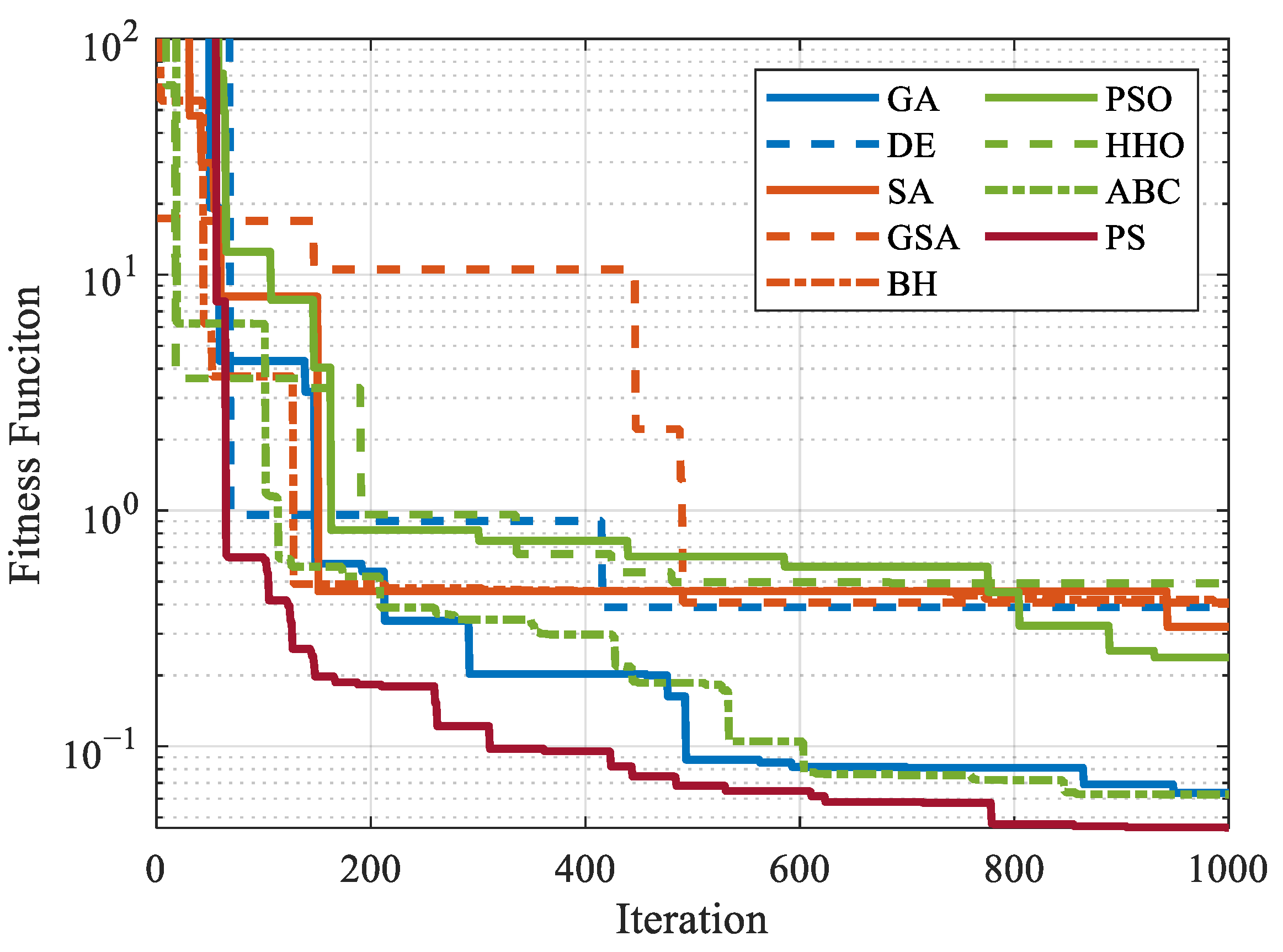
For each algorithm, 10 independent runs were conducted and the runs that converged to the lowest fitness function value were plotted over 1000 iterations, as shown in Figure 6. It should be noted that the scale is logarithmic. As observed, although the non-metaheuristic PS yielded the best result, the metaheuristic ABC and DE followed closely with commendable performances. Fitness function values that converged were below 1 for all algorithms. Decision analysis is necessary to select the most suitable method among these outputs, as individual behaviors may vary slightly despite similar fitness function values. The optimal approach for this evaluation is the statistical assessment of the algorithms.

Table 5. Comparison of optimization algorithms.

	GA	DE	SA	GSA	BH	PSO	HHO	ABC	PS
$t_{min}$ [s]	1579.3	1882.7	1259.6	1553.1	1903.1	1562.6	1505.2	1385.3	1328.6
$t_{max}$ [s]	1936.3	2241.8	1371.5	1844.6	2379.6	1995.5	2251.7	1758.8	1851.3
$F_{min}$	0.0635	0.1540	0.3210	0.4077	0.3010	0.0991	0.4916	0.0626	0.0451
$F_{STD}$	0.1957	0.0878	0.1565	0.3983	0.2542	0.0648	0.4210	0.1282	0.1568
$f_1={\omega }_1$	194.77	182.03	215.21	190.87	209.23	192.92	180.96	186.90	196.45
$f_2=M$	21.71	23.35	26.93	28.39	26.76	22.81	29.14	21.03	20.25
$f_3=F_1$	688.87	447.62	690.78	1027.4	2095.2	694.42	1347.9	326.79	416.71
$f_4=F_2$	144.51	33.06	47.27	57.00	354.45	111.15	567.42	74.08	29.09
$f_5=F_3$	74.07	119.94	243.61	551.71	733.24	90.96	345.75	125.73	75.02
$f_6={\delta }_1$	0.020	0.012	0.013	0.029	0.054	0.019	0.0571	0.007	0.008
$f_7={\delta }_2$	0.023	0.019	0.013	0.040	0.073	0.026	0.0627	0.008	0.012
$f_8={\delta }_3$	0.002	0.005	0.010	0.023	0.028	0.002	0.0129	0.004	0.003

presents the standard deviations alongside the optimal values obtained from the algorithms. Having a lighter rotor correlates with reduced potential energy and leads to a more efficient rotor design. The results indicate that the PS algorithm produced the lightest rotor.

Another critical aspect for turbomachines is minimizing the variation in blade tip clearance values within the operational range. Variations in blade tip clearance directly impact the performance of the turbomachine. In this context, the ABC algorithm yielded the rotor with the least deflection.

Considering that turbomachines operate at high speeds, the magnitude of forces experienced in the bearings is crucial. Repeated exposure to these forces can significantly affect the operational lifespan of the machine. The results show that the BH, GSA, and HHO algorithms recommended a rotor structure that experienced high forces on the first bearing.

Another important consideration is to keep the natural frequency as far away as possible from the operating speed range. In contrast, the SA algorithm proposed the rotor with the highest natural frequency. Regarding standard deviation, the PSO algorithm provided the most reliable results, while HHO exhibited the highest standard deviation among the optimization algorithms.

The preferred algorithm should closely approach all objective functions with a low standard deviation. Since optimization problems generally involve time-consuming improvement processes, it may not be feasible to test all algorithms comprehensively in real-world scenarios. If metaheuristic algorithms are to be evaluated, ABC can be considered the best performer. However, it should not be overlooked that PS also demonstrated superior performance, outperforming many metaheuristic algorithms.

After evaluating the fitness function, a detailed assessment of each algorithm’s best solution was conducted. The optimal solutions were evaluated in terms of their frequency response function (FRF) and rotordynamic characteristics, as discussed in the subsequent subsections.

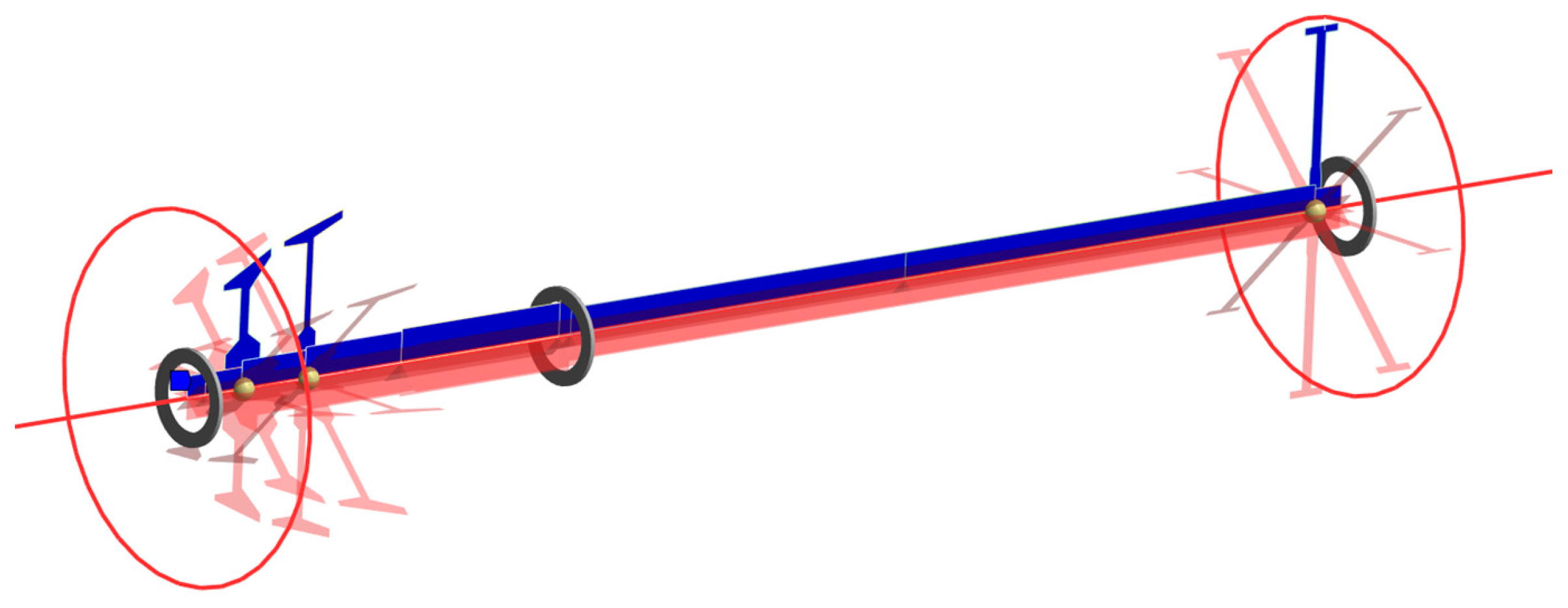
5.1. Consideration of Rotordynamic Behavior

When a rotor spins, it undergoes gyroscopic separation into forward whirl and backward whirl at its natural frequency. The backward whirl frequency primarily excites damping-related structures, while the forward whirl frequency triggers unbalance-induced lateral modes. Therefore, it is desirable for the forward whirl frequency to remain outside the operating speed range. For the optimization study, the operating speed was set at 160 Hz. With a 25% margin, the forward whirl frequencies should ideally be 200 Hz (12,000 RPM) or higher. Indeed, as observed in Figure 7, the best results from all optimization algorithms exceed this margin. Although gyroscopic behaviors vary from model to model, all models meet the desired criteria. The key consideration is that rotors achieving this frequency with the lowest mass are more valuable, as a lightweight rotor corresponds to a significant cost parameter. For instance, although the critical speed of the model suggested by HHO meets the operating speed margin, it does so with a rotor that is 9 kg heavier than the one proposed by PS.

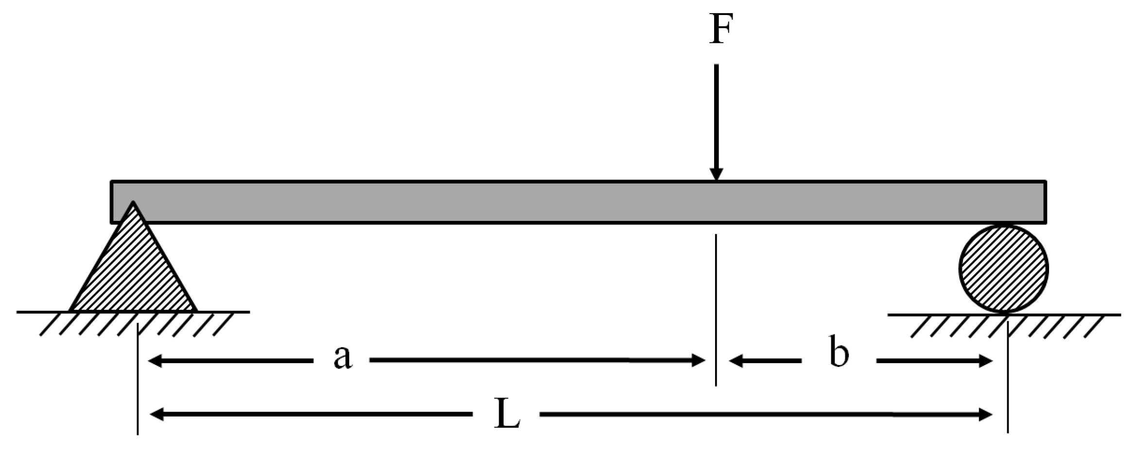
The disks shifted toward the bearings as a result of the optimization. Considering $F=m·e·{\omega }^2$, it is likely that the radial misalignment on the disk will be greater than that on the shaft. To minimize the deflection caused by this force and increase the stiffness, the disks approaching the bearings as much as possible align with Equation (30). Indeed, as the value of b in Equation (30) decreases, the deflection decreases and the shaft stiffness increases.

$${\delta }_{max}={\displaystyle \frac{Fb(3L^2-4b^2)}{48EI}}$$

(30)

Here, δ represents the maximum deflection of the beam, F denotes the unbalanced force, L is the total length of the beam, b is the distance to the load application point, E is the modulus of elasticity, and I is the area moment of inertia of the beam. To aid in the understanding of these expressions, a graph is provided in Figure 8.

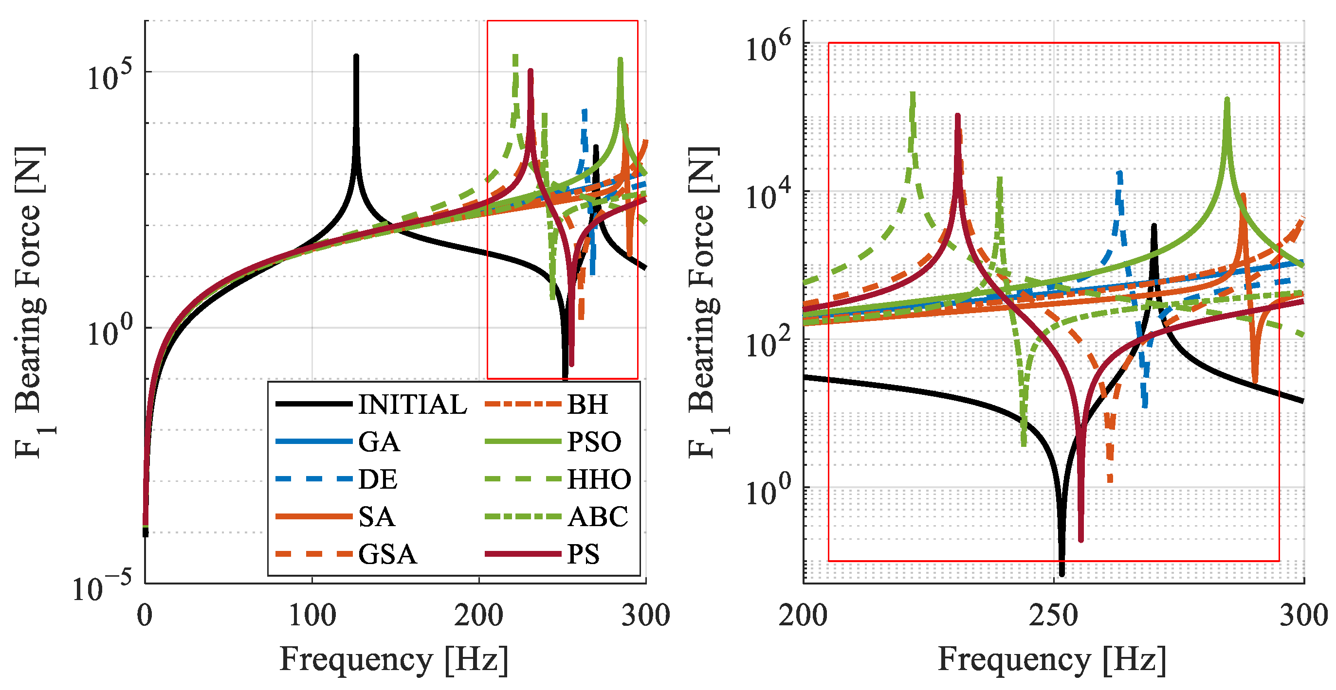
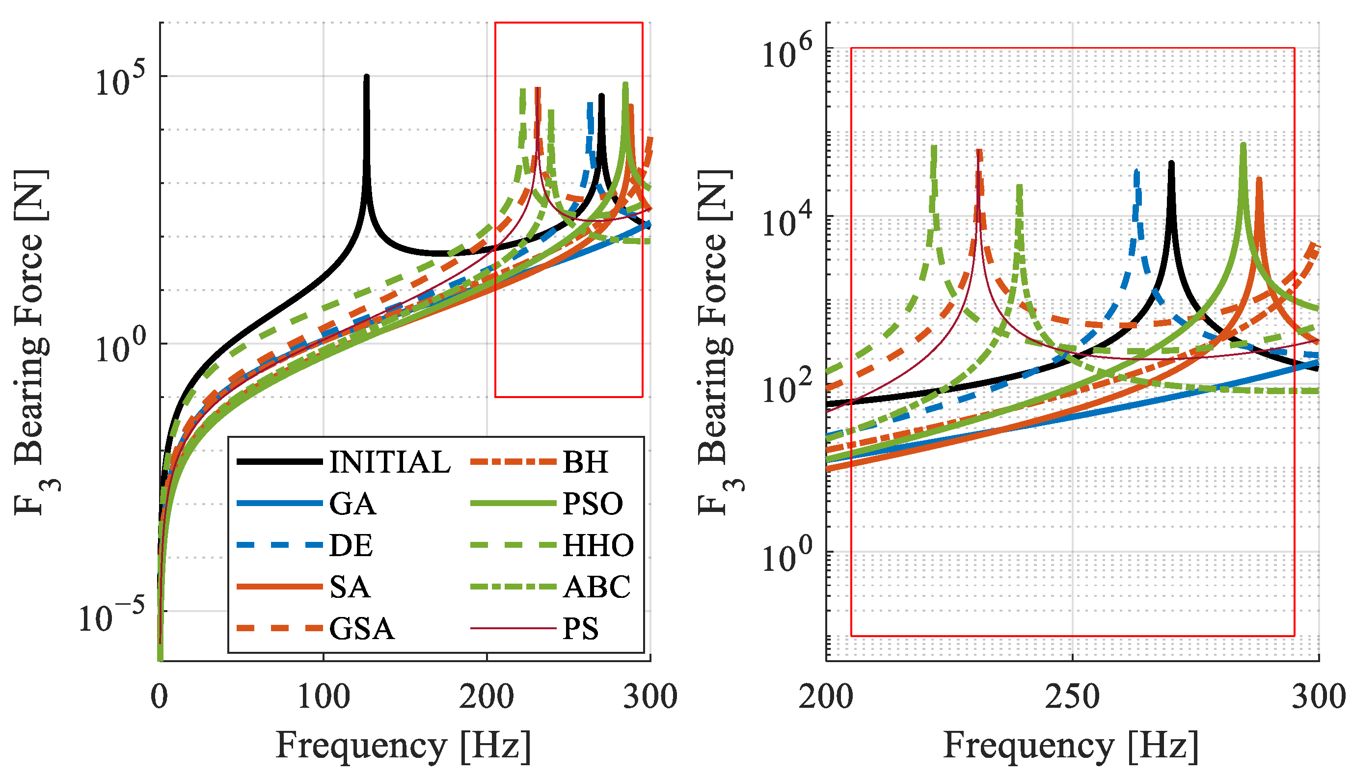
5.2. Frequency Response Function for Bearing Forces

For the force criterion, the target is to observe forces below 5000 N on the bearings. When examining the asymptotic responses, the general trend shows improvement in the response distributions. Figure 9, Figure 10 and Figure 11 illustrate that, compared to the initial rotor structure, the natural frequency due to gyroscopic effects increased, and the initial amplitude values are lower. The entire FRF range for each bearing and a close-up view of the clustered values at higher frequencies are provided.

When examining the overall responses, the ABC algorithm stands out. Its peak values are generally lower than those of other algorithms. Following closely, the SA algorithm also shows lower values, but it proposes a rotor structure that is 6 kg heavier than that suggested by the ABC algorithm.

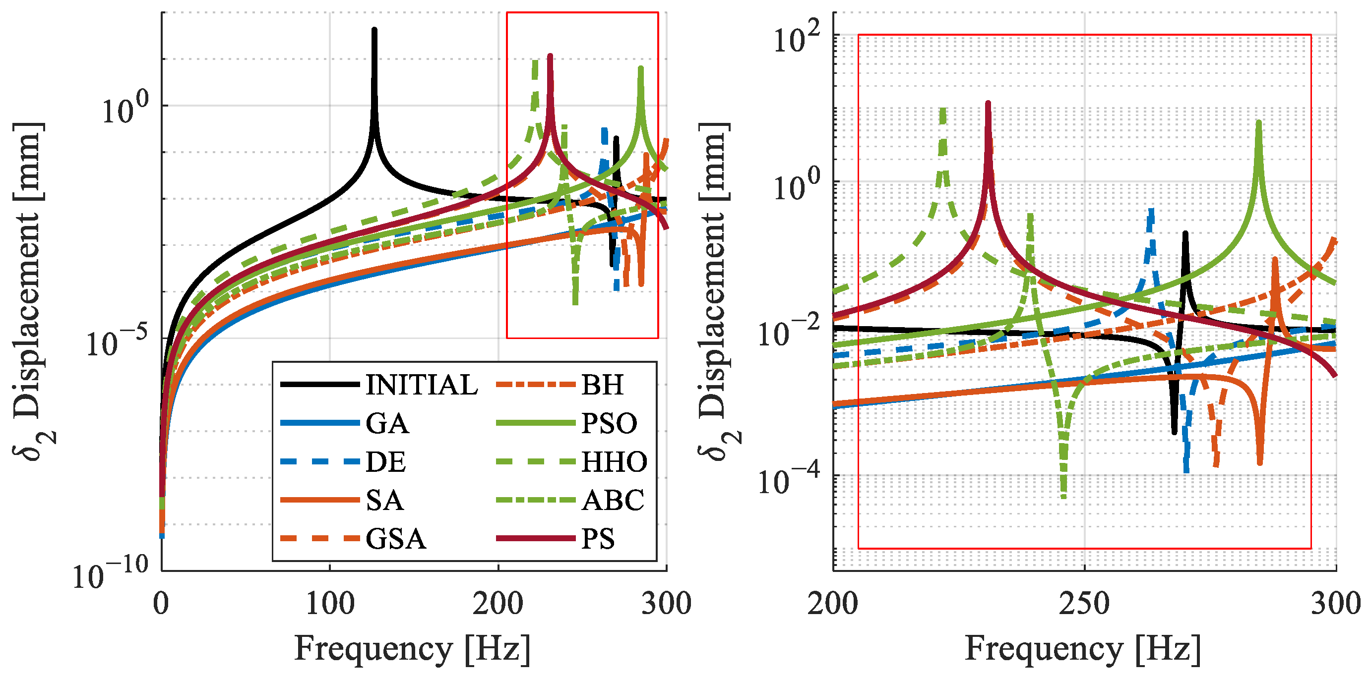
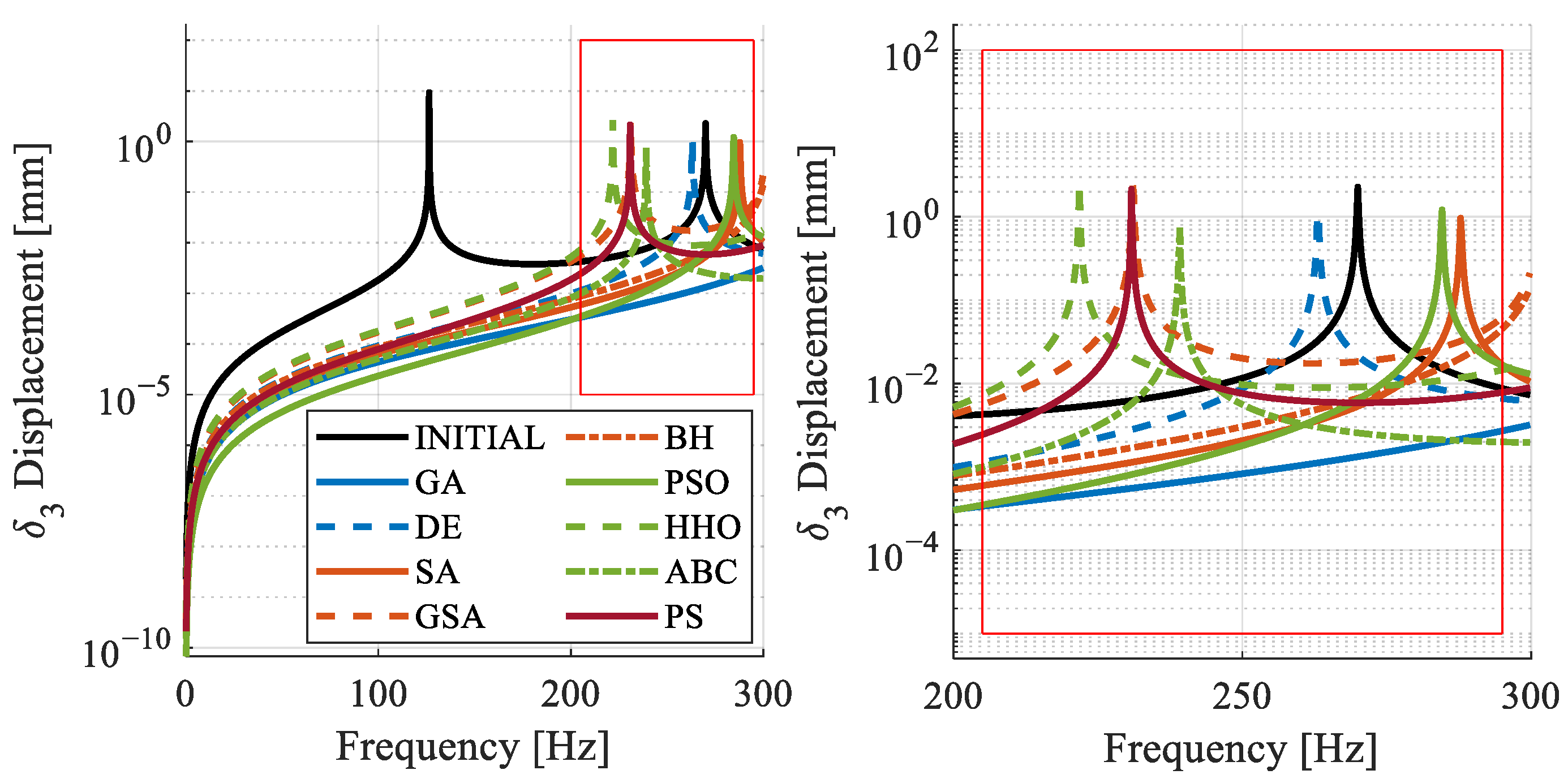
5.3. Frequency Response Function for Disk Displacements

For displacement, the desired criterion is to maintain values below 1 mm on each disk. The obtained displacement values show similarities to the force values observed on the bearings as in Figure 12, Figure 13 and Figure 14. The behavior of the FRF obtained from the algorithms indicates an overall improvement.

5.4. Time Consumption of Optimization Algorithms

Evaluating the FRF response for disk deflection and bearing force resulted in some time loss per iteration, but the most time-consuming aspect was the inner loops of the optimization algorithms. When analyzed independently, faster results were obtained for each unit. The primary advantage of using the TMM over the FEM is evident here; performing such a cycle with the FEM to obtain both natural frequency values and FRF response would be significantly more time-consuming. The efficiency of the TMM in terms of time was more thoroughly examined by comparing the FEM’s results with the TMM’s outcomes for optimized ABC geometries.

When considering the time performance, as illustrated in Figure 15, the SA algorithm delivered the fastest results, while the BH algorithm was the slowest. Additionally, the variability in solution times observed with HHO is thought to be related to its exploration and exploitation processes. Notably, the algorithms that produced the best outcomes—ABC, DE, and PS—demonstrated similar time values. However, the variation in time performance is not necessarily attributable to the inspiration method, suggesting that classifying metaheuristic methods based on their inspiration may not always correlate with similar performance outcomes.

6. Assessment of FEM and TMM with Optimized Design

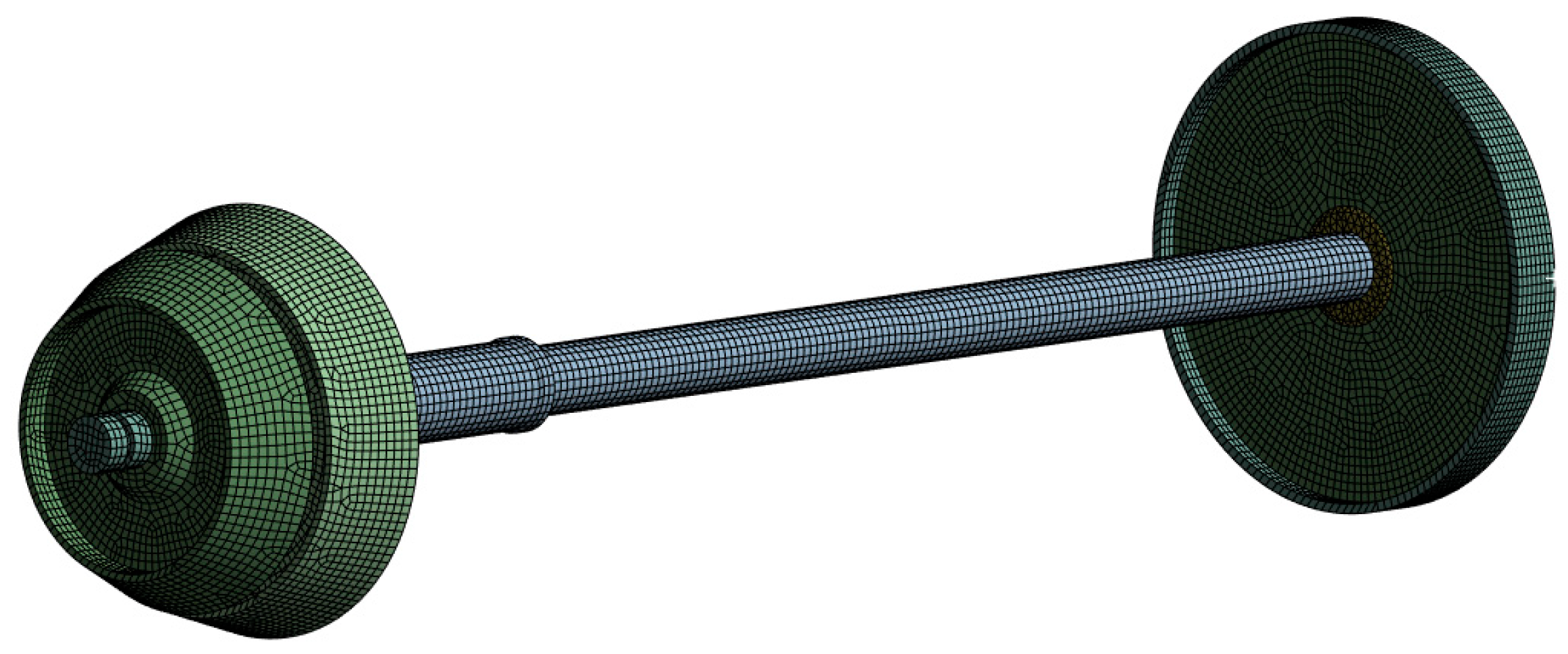
To demonstrate the accuracy of the TMM’s results we obtained, a comparison with the FEM was conducted in this section. For this comparison, a 3D model was initially created as shown in Figure 16 over optimized ABC geometry. Utilizing the geometric properties of this 3D model, a 2D axisymmetric model was then generated using Ansys, as depicted in Figure 17. The use of the axisymmetric model was chosen because its mathematical representation is similar to the TMM and it provides the most stable results for rotordynamic modeling in Ansys. The blades on the disks on the rotors were defined as point masses using the MASS21 element. The COMBI214 element type was selected for the bearings. The SOLID272 element type was used for the axisymmetric model. The obtained results demonstrate the high quality and speed of the TMM solutions. The comparison focused on evaluating the convergence of frequency response and natural frequency results with respect to different mesh sizes and solution times.

6.1. Natural Frequencies

The 2D axisymmetric geometry was created as shown in Figure 17. By adding mass and bearing elements to this model, a general axisymmetric structure was obtained. Two types of analyses were performed on this model depending on the mesh quality. The first analysis used a 1 mm mesh size, while the second used a 10 mm mesh size. A comparison of the results obtained from these analyses with those from the TMM is shown in

Table 6. TMM and FEM natural frequency comparison.

Mode #	TMM	FEM—10 mm	% Diff. with 10 mm	FEM—1 mm	% Diff. with 1 mm
1	184.12	188.55	2.34	183.81	0.16
2	340.79	348.08	2.09	339.16	0.01
3	483.71	494.08	2.10	480.62	0.64
Time [s]	0.107	2.6	×24.29	9.9	×92.52

.

The results obtained from the TMM are closely aligned with analytical results, indicating that improving mesh quality leads to the convergence of the FEM’s results toward those of the TMM. This convergence occurs because the FEM model representing the rotor structure discretizes the system into stiffness matrix [K] and mass matrix [M]. Consequently, the mass distribution remains dependent on the mesh size due to this discretization. In contrast, the TMM does not perform such discretization; instead, it defines the mass and stiffness expressions within the element matrix in a sinusoidal continuous manner. This approach enables the attainment of results that are not only rapid but also closely approximate the analytical solution, regardless of the number of elements used. Thus, the increase in element quality contributes to the alignment of the FEM’s results with the TMM’s results.

A significant difference in computation time is observed between the two methods. For an FEM model with a mesh size of 10 mm, the solution time differs by a factor of 24.29 compared to the TMM, while at a mesh size of 1 mm, this difference increases to a staggering 92.52 times. This duration will further increase during the examination of the frequency response function (FRF). The FRF analysis involved performing a series of modal analyses discretized according to defined frequencies. Since the natural frequency must be determined at each analysis step as one of the objective functions, this will cumulatively expedite the overall results. Furthermore, as the complexity of the model increases, more elements will be needed to accurately represent the rotor structure. In such cases, the solution speed advantage of the TMM becomes increasingly significant. It is important to note that in this comparison, the rotor was modeled in Ansys as a general axisymmetric structure. Although the solution time may vary for different FEM models, the TMM will maintain its superiority.

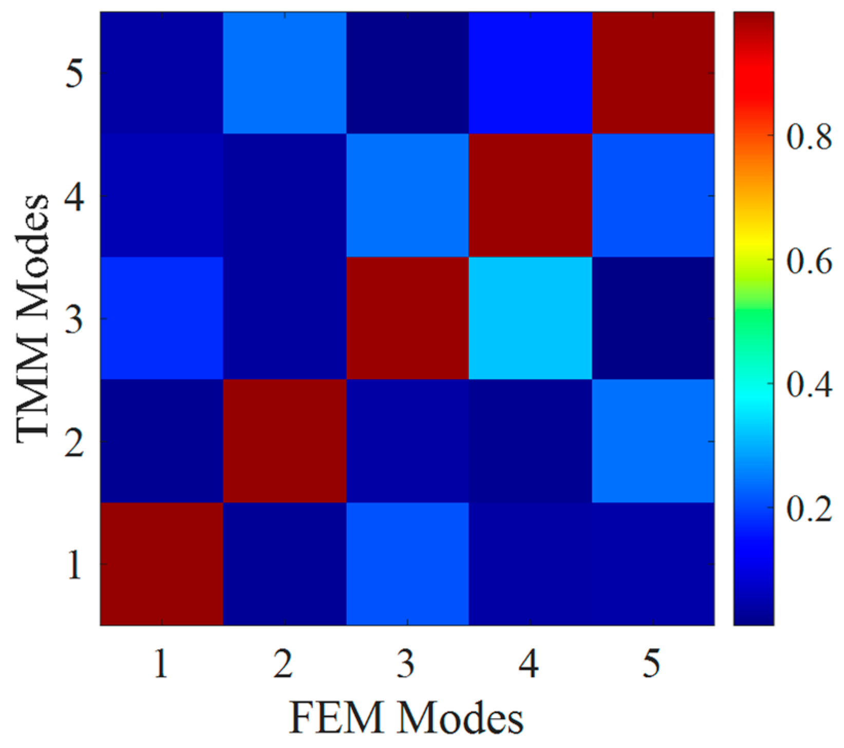
6.2. Mode Shapes

The results from the 2D general axisymmetric model and the TMM for examining mode shape correlation is presented in Figure 18. The first five modes were analyzed, revealing that their modal assurance criteria (MAC) values are close to 1. This indicates a high degree of consistency between the mode shapes obtained from both methods.

6.3. Frequency Response Function

In addition to the natural frequency comparison, the FRF graph was also examined in this model. To ensure a robust comparison and mitigate asymptotic FRF behavior, bearing damping values were increased to 10 Ns/mm. In this context, the comparison of the TMM and FRF graph of the FEM model with different mesh sizes for the third bearing is shown in Figure 19. In this comparison, the frequency band chosen was between 230 Hz and 250 Hz with an interval of 0.1 Hz under the effect of unbalance. Additionally, comparison results in terms of solution time are given in

Table 7. TMM and FEM FRF time consumption comparison for per iteration.

	TMM	FEM—10 mm	FEM—1 mm	Diff. with 10 mm	Diff. with 1 mm
Time [s]	0.099	4.1	214.4	×41.41	×2165.65

. For all three models compared, the amplitude values and the behavior of the FRF curve are quite similar. The slight differences in frequency observed in Table 6 increased slightly with the gyroscopic effect. These small differences are acceptable and demonstrate that the models are working consistently. The main difference is observed when comparing the solution times. If the FRF output is to be used for an objective function, the importance of using the TMM becomes evident because the enhanced element quality of the FEM’s results converge toward the TMM.

7. Conclusions

The evaluation of nine different optimization algorithms highlighted the significant advantages of selecting the most suitable algorithm for accelerating the preliminary design phase and improving decision-making accuracy in complex optimization problems. Although the fitness function values of all optimization algorithms converged below 1, the multi-objective improvement was conducted through different parameters due to the differences in their behavior during the exploration and exploitation processes as stipulated by the NFL theorem. Among these, the metaheuristic ABC and pattern-based PS algorithms achieved commendable results by considering the requirements of all objective functions without focusing solely on improving a single point. Additionally, it should be noted that these two algorithms had relatively good optimization times compared to others, except for SA.

The study successfully achieved a rotor geometry that operates within a 200 Hz margin, avoids any natural frequencies within this range, and minimizes bearing and disk forces as much as possible, all while maintaining a lightweight structure. The optimized rotor geometry, as shown in Figure 16, bears a close resemblance to the benchmark J85-GE, with similarity references drawn from the positions of the compressor and turbines due to the unclear bearing positions in the figure.

Our optimization efforts utilized the CTMM-based rotordynamic solution, which proved to be efficient and effective. The CTMM approach not only matched benchmark geometries with satisfactory time efficiency but also demonstrated its superiority over the FEM in terms of computational time. This reinforces the CTMM’s suitability for robust rotordynamic optimization.

These results indicate that the use of the TMM in other engineering fields where it is already applied will provide an advantage in terms of solution time for optimization studies compared to the FEM. It is important to note that in the optimization problem addressed, the focus is on the force and displacement values on the system rather than the stress distribution at a specific point. While the FEM may maintain its superiority over the CTMM in this regard, significant optimization studies can be conducted using the CTMM.

Future work will focus on further advancing the CTMM tool to tackle more intricate rotordynamic challenges and facilitate rapid iterations. These efforts aim to solidify the CTMM as a versatile and efficient solution for optimizing rotor systems across a wide range of engineering applications.