Studies on Submersible Short-Circuit Blowing Based on Orthogonal Experiments, Back Propagation Neural Network Prediction, and Pearson Correlation Analysis

Abstract

Short-circuit blowing is a crucial technical approach for ensuring the rapid surfacing of submersibles. In order to investigate the law, L₁₈(3⁷) orthogonal experiments based on a proportional short-circuit blowing model test bench were conducted. Subsequently, a Back Propagation Neural Network (BPNN) and Pearson correlation analysis were employed to train the experimental data; further examination of the correlation between individual factors and blowing served as an enhancement to the orthogonal experiments. It has been proved that both multi-factor combinations and personal factors, including blowing duration, sea tank back pressure, gas blowing pressure from the cylinder group, and sea valve flowing area, exert significant influence with Pearson correlation coefficients of 0.6535, 0.8105, 0.5569, and 0.5373, respectively. Notably, the F-ratio for blowing duration exceeds the critical value of 3.24. The statistical evaluation metrics for the BPNN ranged from 10⁻¹ to 10⁻¹², with relative errors below 3%, and achieving a prediction accuracy rate of 100%. Based on these findings, a robust predictive methodology for submersible short-circuit blowing has been established along with recommendations for engineering design and operational strategies that highlight its advantages as well as its initial condition settings.

1. Introduction

In the past few years, the navigational safety of submersibles has garnered increasing and widespread attention. High-pressure blowing is a critical method for ensuring submersible surfacing. Among these applications, the two most prevalent scenarios are rudder jamming during high-speed navigation and emergency procedures in response to flooding compartments [1]. Short-circuit blowing specifically refers to an effective technique for expelling ballast water directly from tanks using compressed gas sourced from a cylinder group, bypassing the gas distribution mechanism. Its efficiency is influenced by various operational factors, including gas pressure and other relevant parameters [2]. Currently, primary methods for studying short-circuit blowing encompass mathematical modeling, numerical calculations, and experiments conducted on actual vessels or dedicated test benches.

In the domain of mathematical modeling and numerical simulations, Computational Fluid Dynamics (CFD) techniques are employed to investigate the formation and evolution of the gas–liquid two-phase interface within ballast tanks during short-circuit blowing, providing a comprehensive analysis of discharge rate variations [1]. Several studies in this area have examined individual operational factors, including the flow area of the sea valve [3], outboard back pressure, high-pressure cylinder group gas pressure, cylinder volume [4], and supply pipelines for both gas and water [5]. Utilizing the Laval nozzle theory, an emergency surfacing motion model for submersibles that incorporates short-circuit blowing was developed. Additionally, a water ingress restriction line within the safety boundary diagram for underwater maneuverability was derived [6]. While these studies offer valuable insights, they lack specific experimental validations and generalizability; due to their omission of comprehensive operational factors, they did not fully encapsulate the physics principles underlying short-circuit blowing.

In the realm of real-ship or bench experiments, an emergency short-circuit blowing test was conducted on a Spanish S-80 submarine, achieving an instantaneous blowing gas pressure of up to 25 (MPa), equivalent to an outboard back pressure at a depth of 2500 m, which poses significant safety risks [7]. Additionally, small-scale emergency gas jet blowing-off bench experiments were performed to simulate the blowing and drainage performance at a depth of 100 m, yielding relative errors in the drainage percentages of 5% and 10%, respectively [8,9]. Experiments utilized a small-scale short-circuit blowing test bench to evaluate the physics principles underlying the Laval nozzle theory and resulted in a relative error of 8% concerning the flow rate from the high-pressure gas cylinder group, an outcome closely linked to the ballast tank drainage percentage [10,11,12]. While data from the real-ship experiments were highly credible, they entailed considerable risk. Conversely, although the small-scale bench experiments can validate theoretical models, their results were constrained by the scale effect and thus lacked substantial guidance for actual ship manipulation or engineering designs. Nevertheless, proportional short-circuit blowing model experiments serve as a method for investigating the performance characteristics of short-circuit blowing in real ships. These test benches simulated gas cylinder deflation and various ballast tank drainage processes to analyze how factors, such as gas cylinder group volume and pressure, and sea valve flow area, influence blowing efficiency. The resulting relative error for peak gas pressure within the ballast tank remained below 15% when the high-pressure conditions did not exceed 15 (MPa) [2,13,14]. However, compared with actual ship short-circuit blowing, this approach does not encompass the full range of operational conditions and overlooks several critical manipulation factors, including outboard back pressure, along with pipeline length and inner diameter, as well as blowing duration.

The above research is summarized in Table 1 below.

Table 1. Recent research on short-circuit blowing or related fields.

Researching Field	Methodology	Disadvantage
Mathematical modeling	Short-circuit blowing within the framework of Laval nozzle theory [6].	Lacking specific experimental evaluations and universality because of ignoring entire manipulation factors.
	Modeling the evolution of gas–liquid two-phase interface during blowing [1].
	Simulation accounting for the flowing area of sea valves in blowing processes [3].
	Simulation incorporating outboard back pressure, high-pressure cylinder group gas pressure, and cylinder volume in blowing scenarios [4].
	Simulation considering both gas and water supply pipelines [5].
Real-ship or bench experiments	Emergency short-circuit blowing tests were conducted on a Spanish S-80 submarine [7].	Too risky.
	Experiments performed at a depth of 100 (m) [8,9].	Restriction of scale effect.
	Small-scale experiments utilizing a short-circuit blowing test bench [10,11].
	Proportional model tests for short-circuit blowing analysis [2].	Incomplete working conditions, ignoring certain factors.

This paper aims to investigate the influence of various manipulation factors on blowing, with the contributions delineated as follows:

• First, in Section 2, seven detailed influencing factors across three levels of high-pressure short-circuit blowing are identified, and a corresponding proportional model test bench is constructed, as well as L₁₈(3⁷) orthogonal experiments;
• Second, in Section 3, extreme variance and standard variance analyses yield correlation coefficients for blowing duration (0.6535), sea tank back pressure (0.8105), gas blowing pressure from the cylinder group (0.5569), and sea valve flowing area (0.5373). Notably, the F-ratio for blowing duration exceeds the critical value of 3.24;
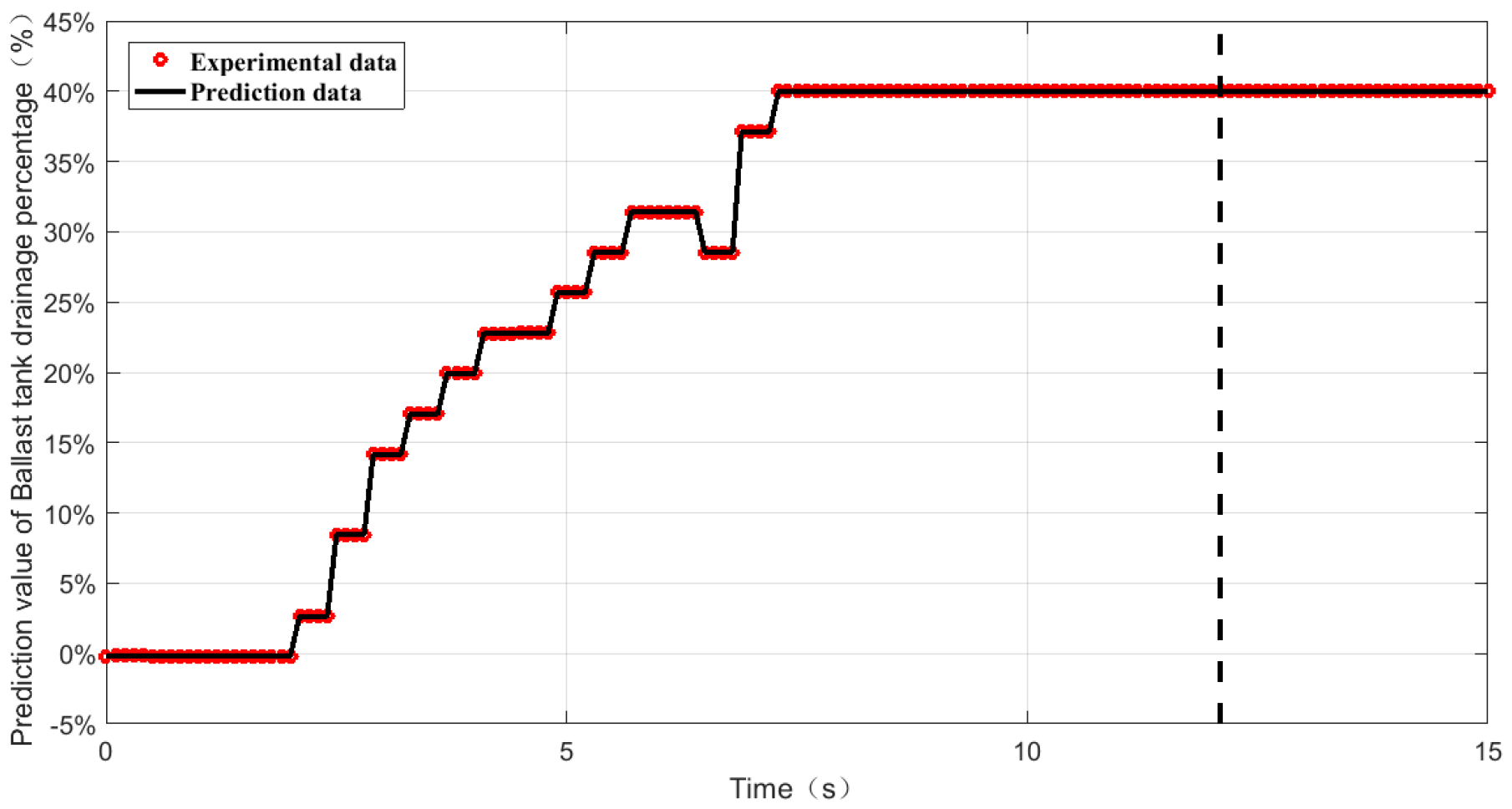
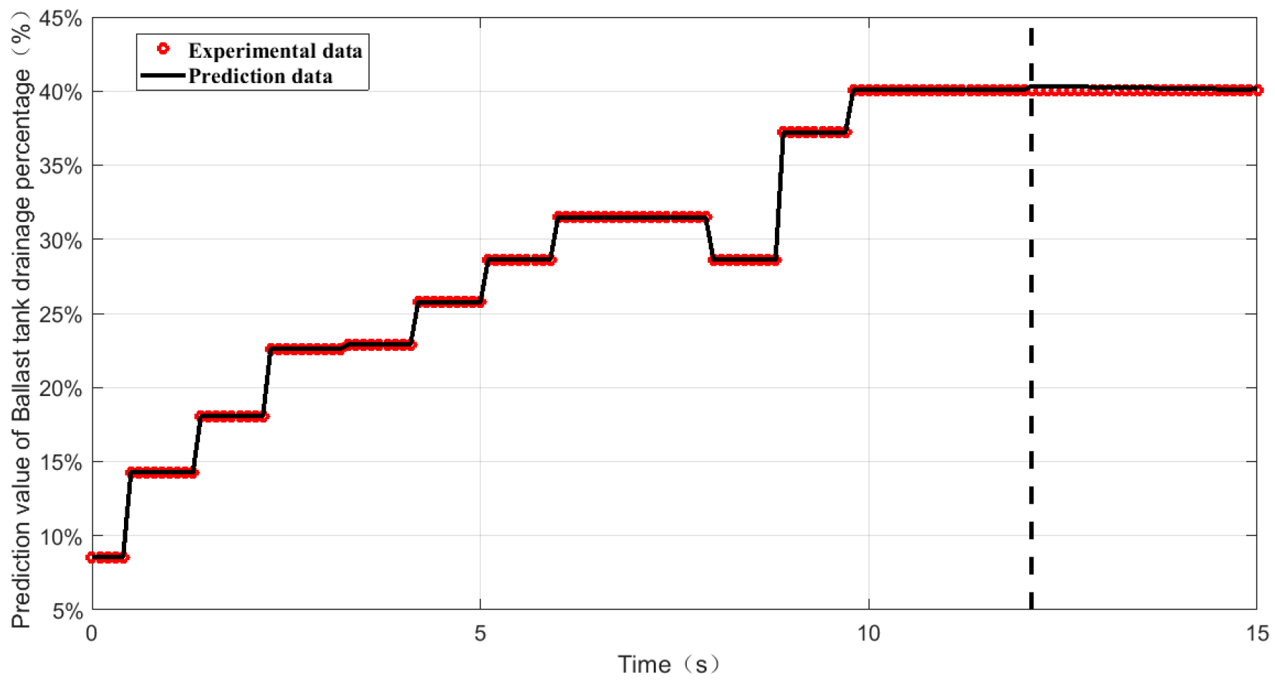
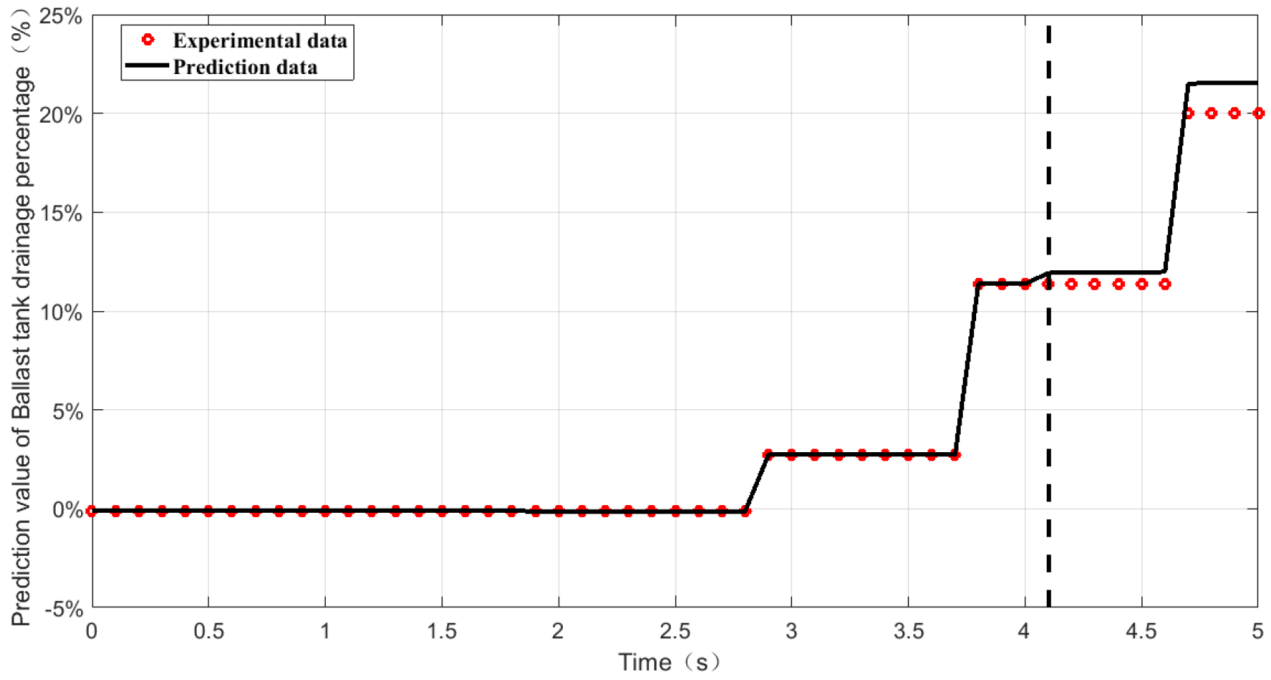
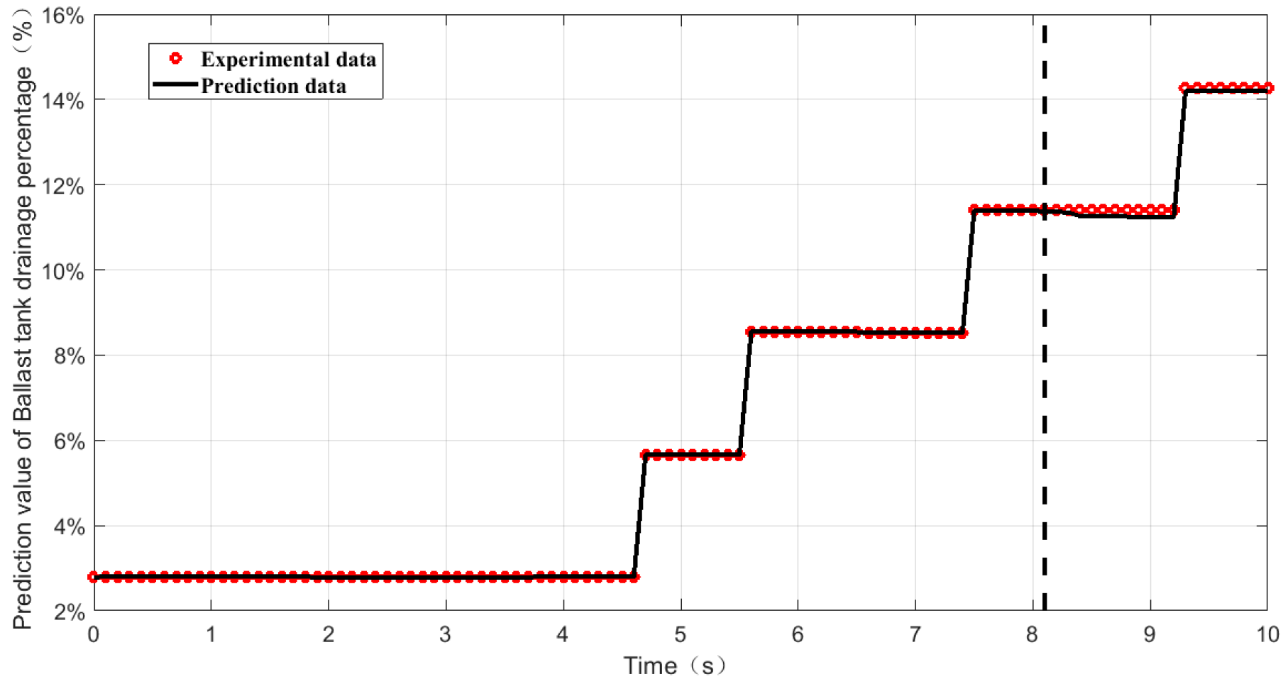
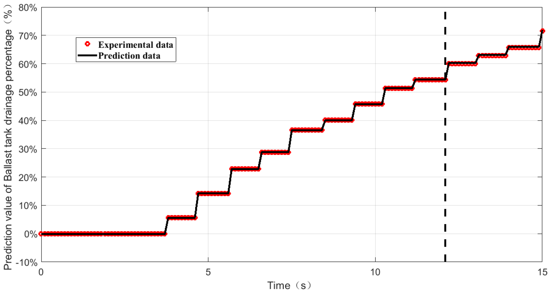
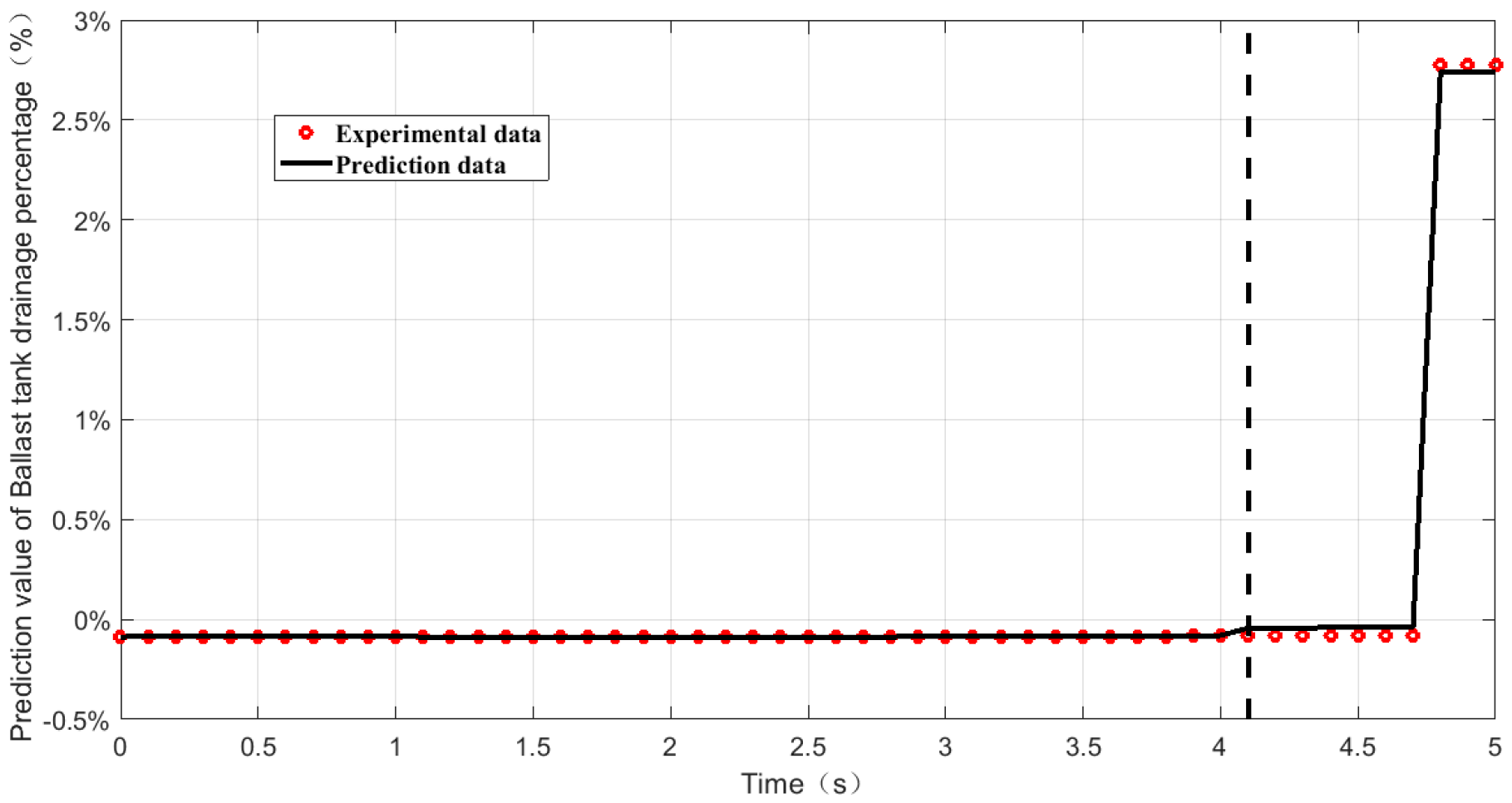
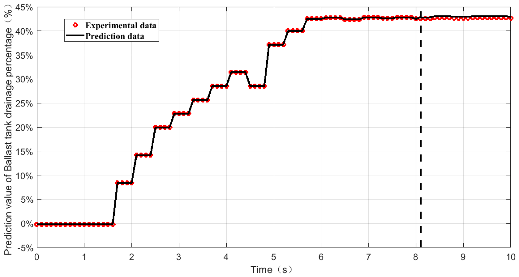
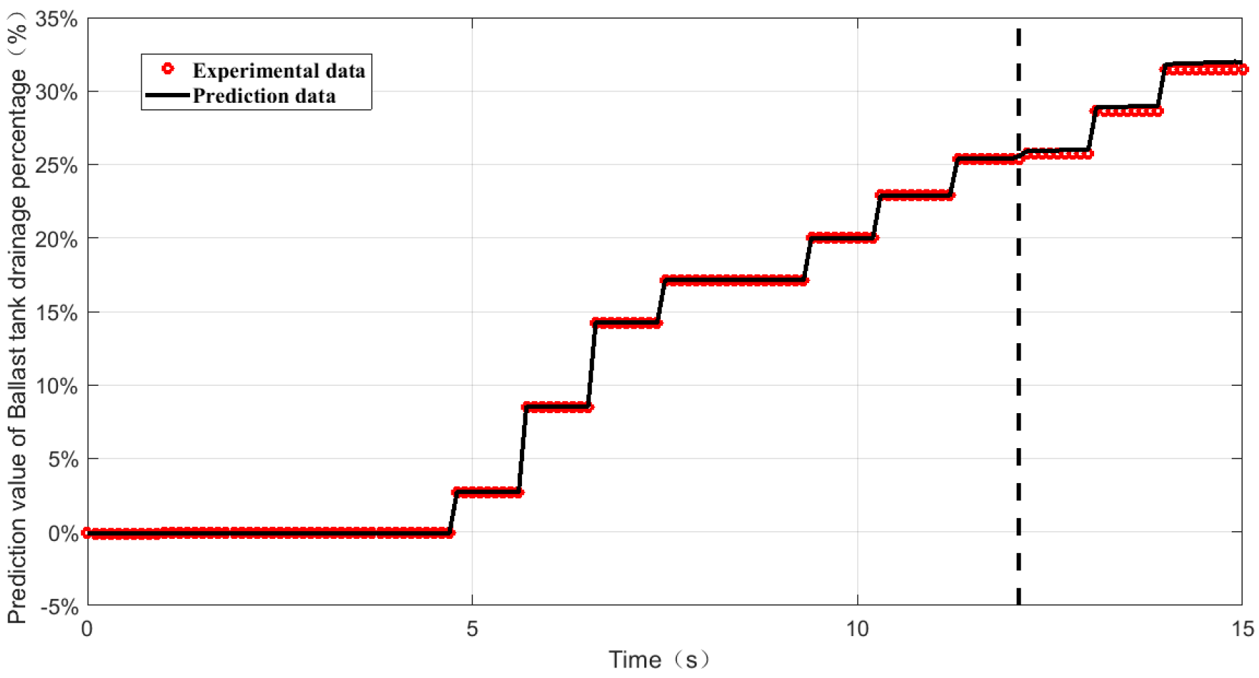
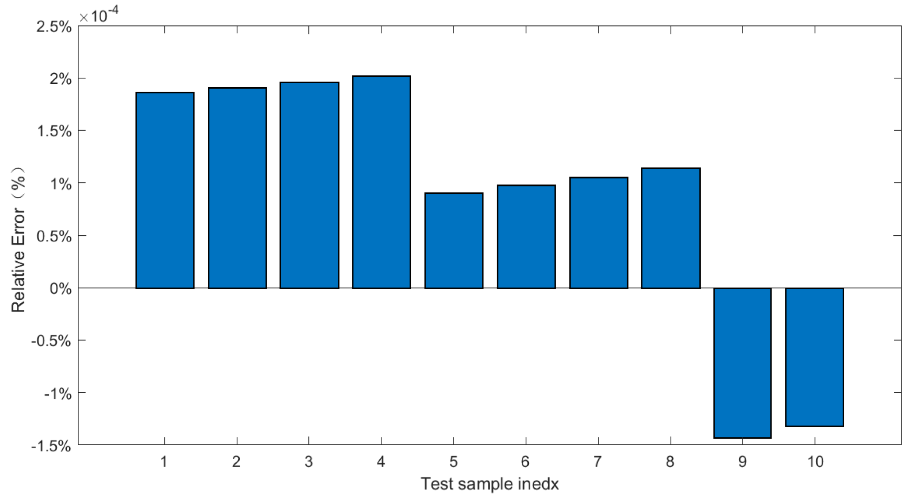
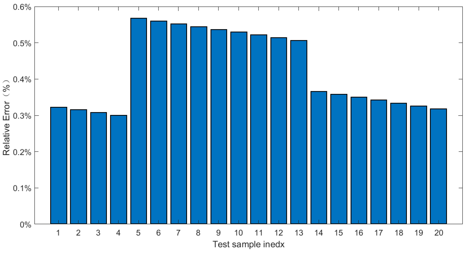
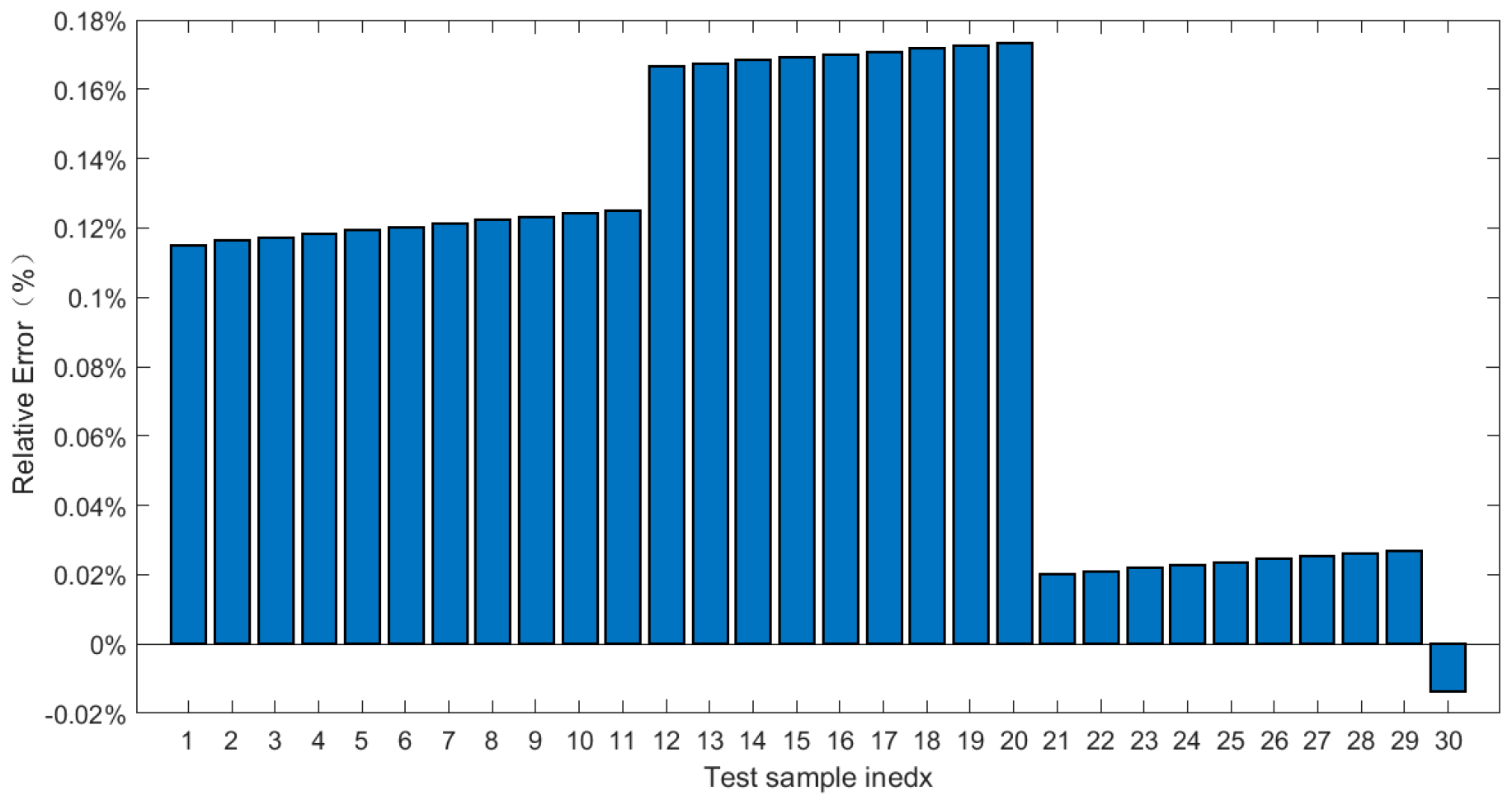
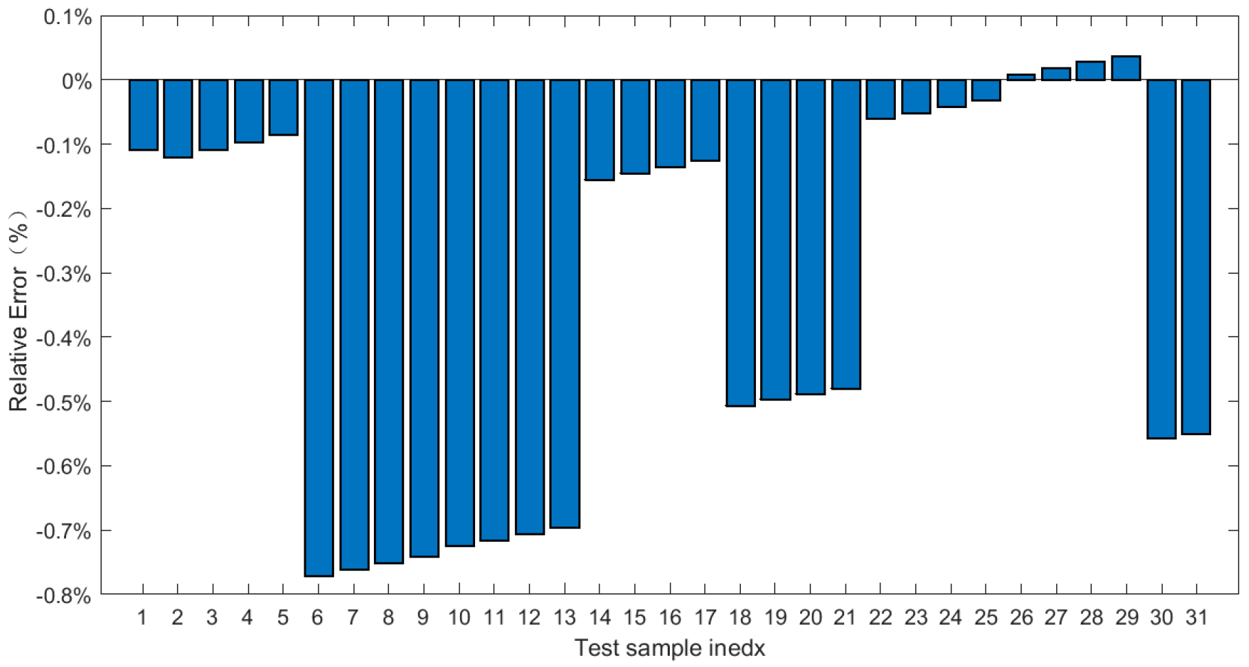
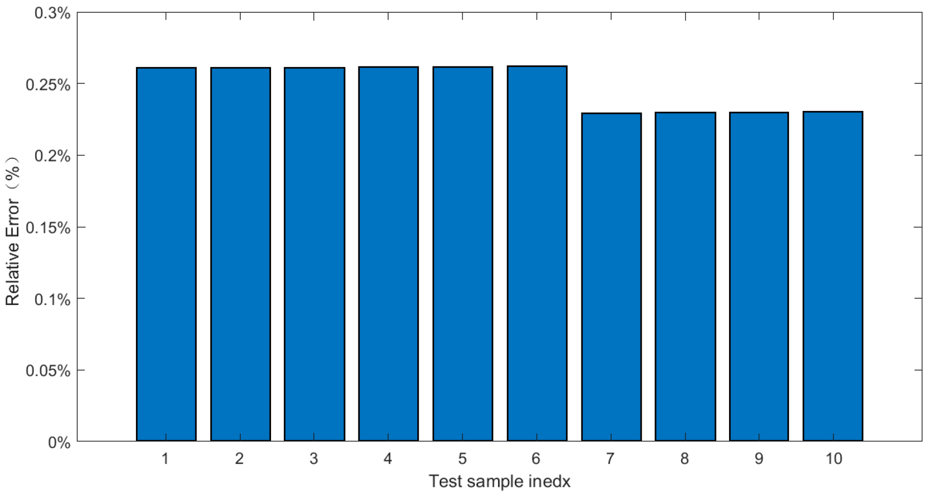
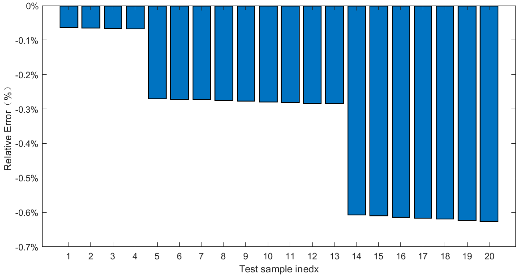
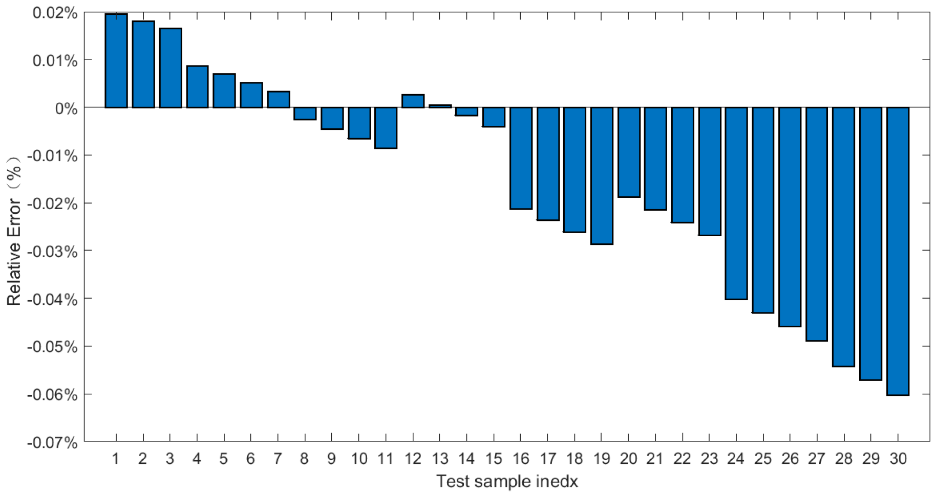
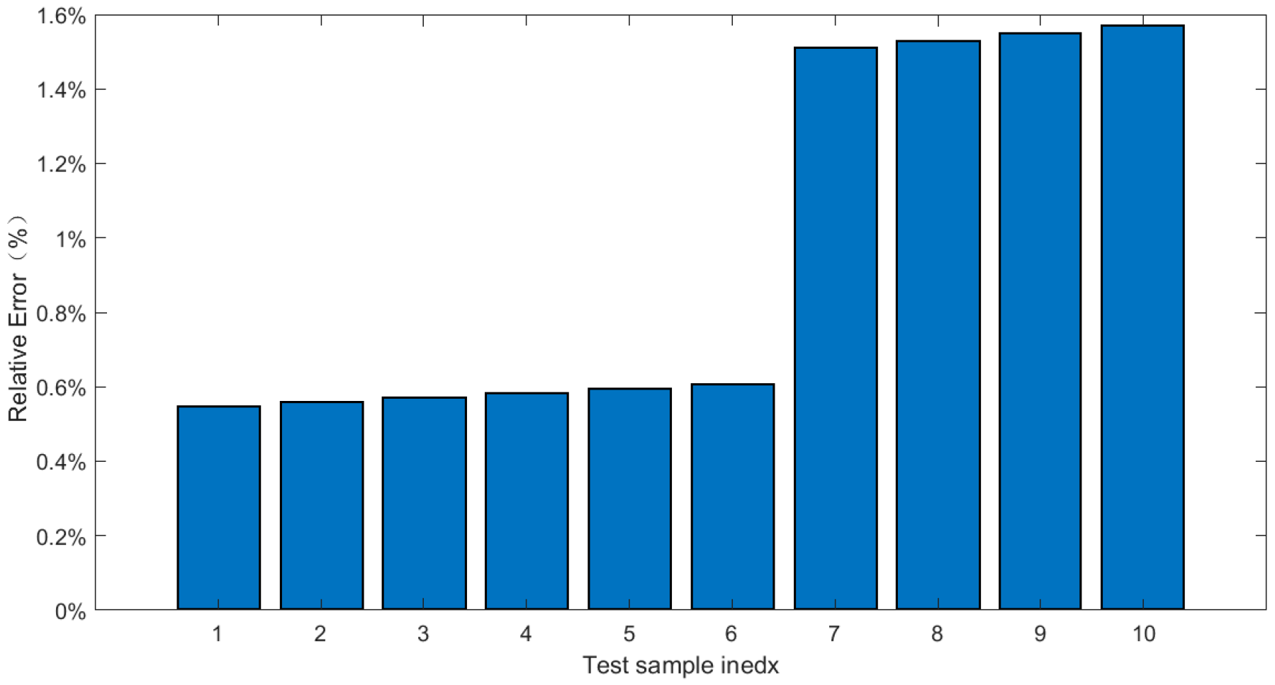
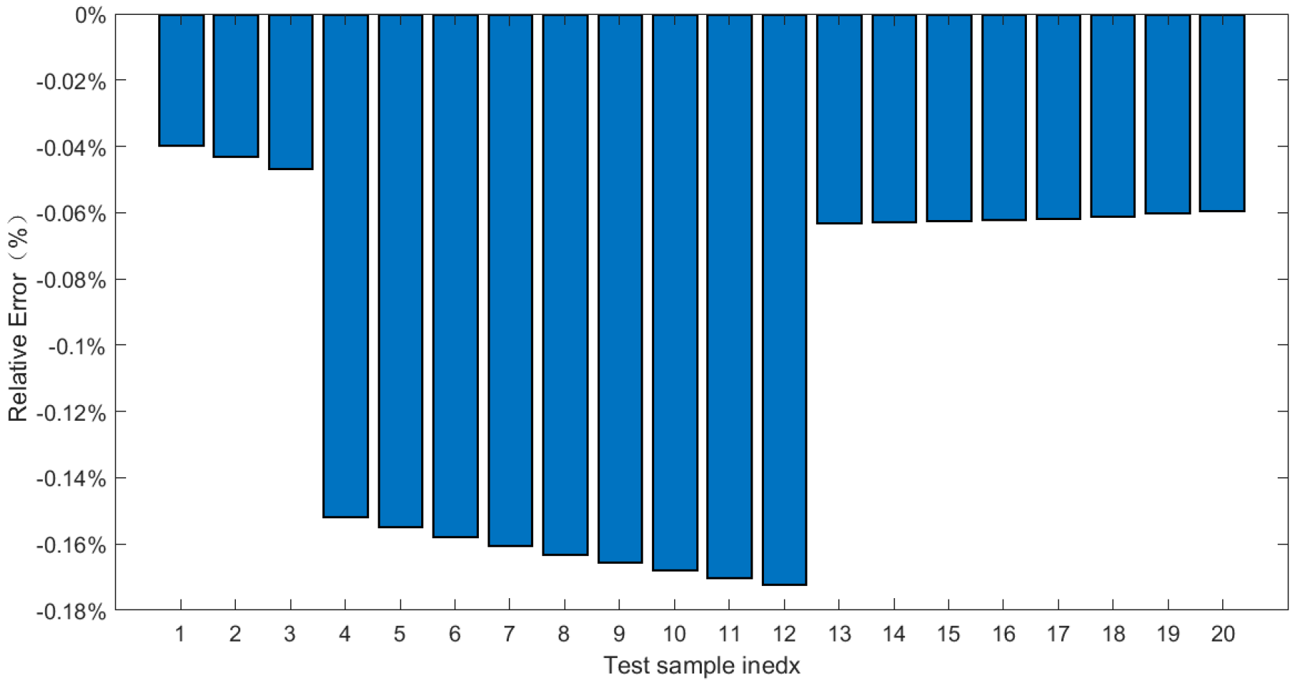
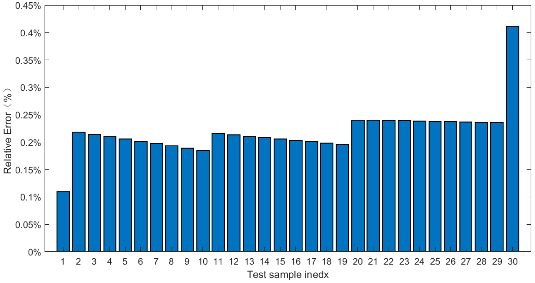
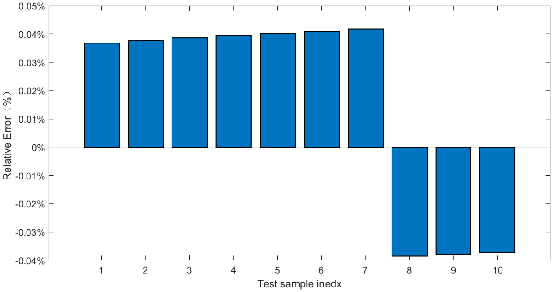
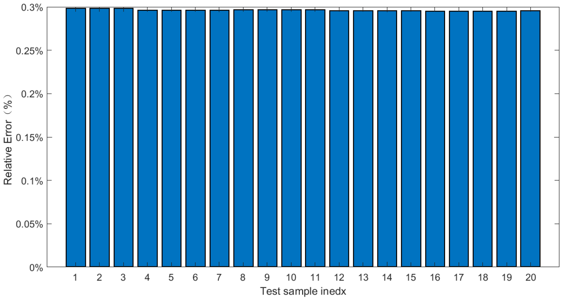
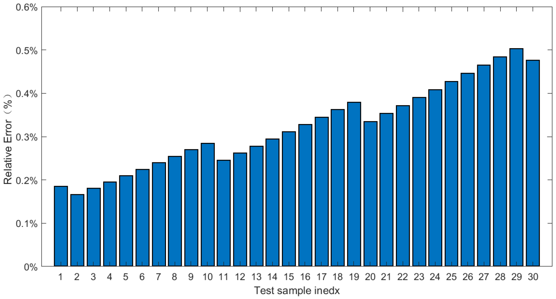
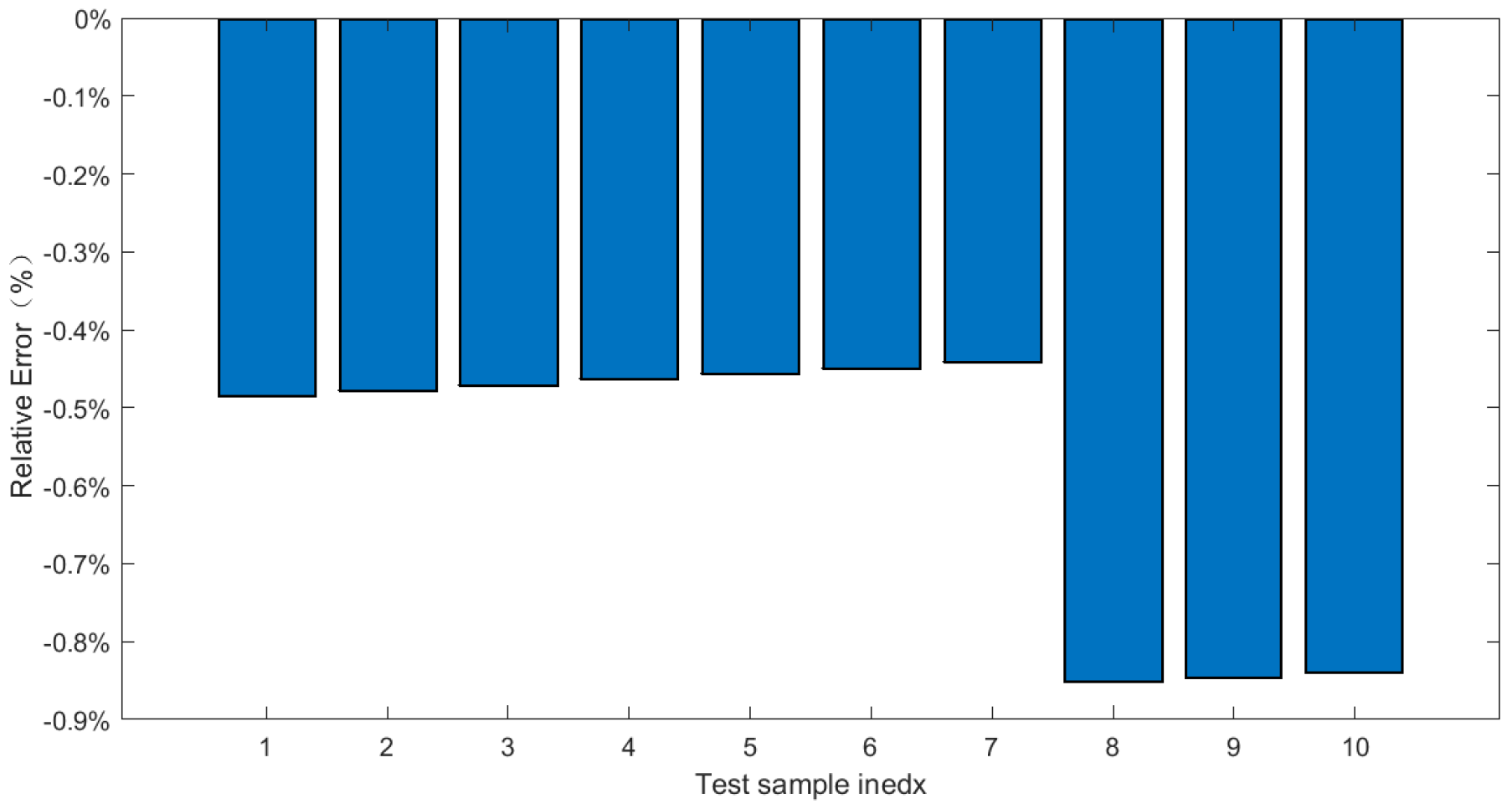
• Third, in Section 4.1, the orthogonal experimental data are trained using a BPNN, resulting in statistical indicators ranging between 10⁻¹ and 10⁻¹², with relative prediction errors below 3% and an accuracy rate of 100%;
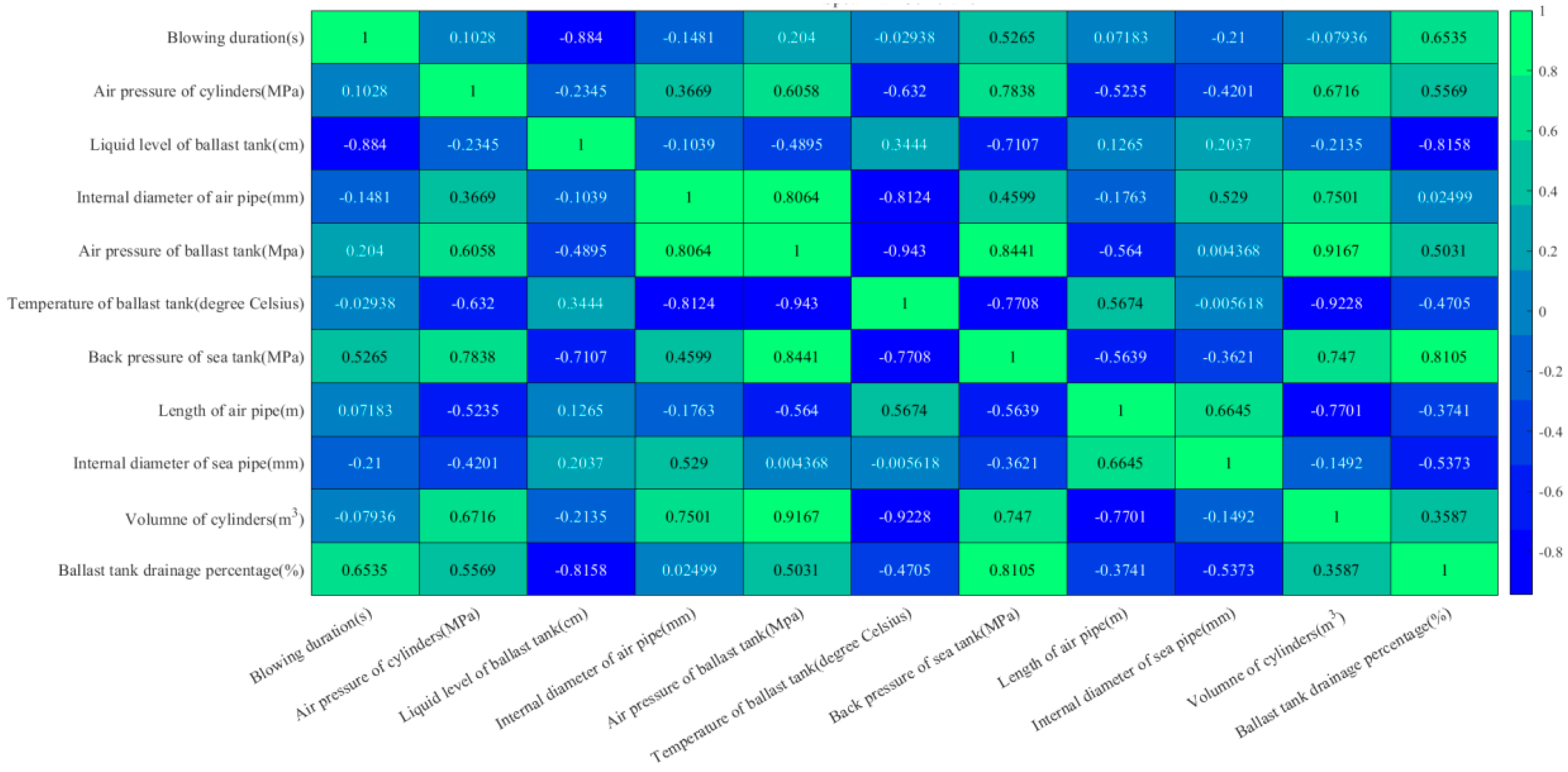
• Fourth, in Section 4.2, Pearson correlation analysis based on orthogonal experimental data is performed to explore the correlation coefficient between individual factors and blowing performance, proving significant insights that complement our findings from the orthogonal experiments.

2. Proportional Short-Circuit Blowing Model Test Bench and Orthogonal Experiment Design

A proportional short-circuit blowing model test bench was constructed based on real ship parameters to investigate the various manipulation factors affected at different blowing levels through orthogonal experiments.

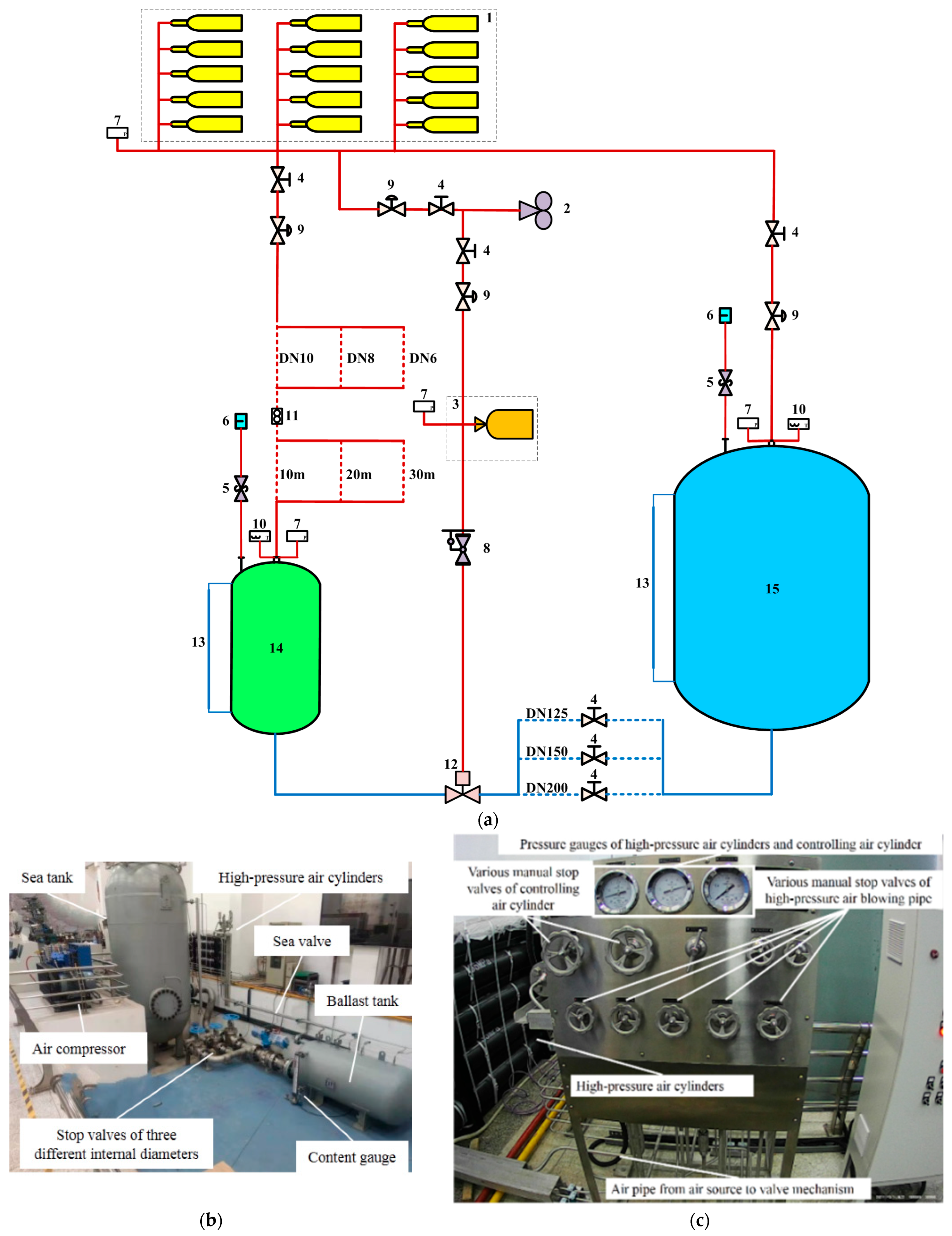
2.1. Detailed Setup of Model Test Bench

The test bench comprised a gas cylinder group, an air compressor, a high-pressure gas cylinder group, and a gas distribution mechanism, along with both the sea tank and ballast tank. Notably, the ballast water tank and sea tank were positioned between sea valves of varying diameters. The air compressor inflated the gas cylinder group while simultaneously pressurizing the sea tank’s top to create back pressure. Upon the initiation of blowing, gas from the cylinder group flew into the ballast tank via the gas supply pipeline, displacing water into the sea tank through the sea valve. A diagram of the proportional short-circuit blowing test bench for submersibles is presented in Figure 1, with its main parameters detailed in Table 2.

Figure 1. Proportional short-circuit blowing test bench of submersible. 1—high-pressure (Hp) air cylinder, 2—Hp air compressor, 3—control air cylinder, 4—stop valve, 5—safety valve, 6—muffler, 7—pressure gauge, 8—relief valve, 9—electric control valve, 10—thermometer, 11—air flow meter, 12—sea valve, 13—content gauge, 14—ballast tank, 15—sea tank. (a) Principle of the test bench. (b) Overall layout of test bench. (c) Valve mechanism of test bench.

Table 2. The main parameters of the experimental bench.

Index	Apparatus	Main Parameters	Remark
1	Air compressor	Maximum air inflation pressure: 20.0 (MPa)
2	Gas cylinder group	Maximum air working pressure: 35 (MPa) Volume: 750 (L)	Gas source for blowing and back pressure in the sea tank
3	Ballast tank	Volume: 1.2 (m3) Pressure handling capacity: 7 (MPa)
4	Sea tank	Volume: 13 (m3) Pressure handling capacity: 5 (MPa)	The back pressure exceeds the maximum working depth of the actual ship.
5	Gas supply pipeline	Three length specifications available: 10 (m), 20 (m), and 30 (m)	The inlet is equipped with three replaceable pipe sections with internal diameters of 6 (mm), 8 (mm), and 10 (mm), each measuring 0.3 (m) in length.
6	Sea pipeline	Internal diameters available: 125 (mm), 150 (mm), and 200 (mm)	Connection between the ballast tank outlet and seawater tank inlet.

2.2. Orthogonal Experiment Design

Compared with the test bench referenced in [2], the manipulation factors for this setup included the volume and pressure of the gas cylinder group, the length of the gas supply pipeline, the inner diameter of the sea valve, the blowing duration, the inner diameter of the gas supply pipeline, and the back pressure from the sea tank. Each factor was assessed at three different levels. According to the permutation and combination principle, a total of 3⁷ = 2187 experiments could be conducted, which represents a substantial number.

The orthogonal experimental method served as an efficient, rapid, and cost-effective evaluation method that was particularly well-suited for multiple factors with various levels. By judiciously selecting orthogonal experiments, it was possible to achieve more accurate and reliable results while minimizing the trial numbers [15]. In this bench, the orthogonal experiment table L₁₈(3⁷) was constructed. Here, the level number was 3, while the factor number was 7, resulting in a total of 18 experiments, as detailed in Table 3. The ballast tank drainage percentage was chosen as a measure for evaluating blowing effectiveness. The seven manipulation factors are denoted by A to G with their respective three levels represented numerically as follows:

Table 3. Orthogonal experiments.

Index of Experiment	The Impacted Factors
	A	B	C	D	E	F	G
1	1	1	1	1	1	1	1
2	1	2	2	2	2	2	2
3	1	3	3	3	3	3	3
4	2	1	1	2	2	3	3
5	2	2	2	3	3	1	1
6	2	3	3	1	1	2	2
7	3	1	2	1	3	2	3
8	3	2	3	2	1	3	1
9	3	3	1	3	2	1	2
10	1	1	3	3	2	2	1
11	1	2	1	1	3	3	2
12	1	3	2	2	1	1	3
13	2	1	2	3	1	3	2
14	2	2	3	1	2	1	3
15	2	3	1	2	3	2	1
16	3	1	3	2	3	1	2
17	3	2	1	3	1	2	3
18	3	3	2	1	2	3	1

• First, A signifies the gas cylinder group volume with three levels: 1–250 (L), 2–500 (L), and 3–750 (L);
• Second, B denotes the gas supply pipeline length across three levels: 1–10 (m), 2–20 (m), and 3–30 (m);
• Third, C refers to the sea valve as the inner diameter at three levels: 1–125 (mm), 2–150 (mm), and 3–200 (mm);
• Fourth, D indicates the blowing duration with three options: 1–5 (s), 2–10 (s), and 3–15 (s);
• Fifth, E represents the inner diameter measurements for the gas supply pipeline and the three levels 1–6 (mm), 2–8 (mm), and 3–10 (mm);
• Sixth, F corresponds to the blowing pressure from the gas cylinder group across the pressures 1–10 (MPa), 2–15 (MPa), and 3–20 (MPa);
• Lastly, G pertains to the back pressure within the sea tank measured at 1–0.2 (MPa), 2–0.5 (MPa), and 3–1.0 (MPa).

3. Orthogonal Experimental Data Analysis

Following the acquisition of results from the L₁₈(3⁷) orthogonal experiments, two statistical analysis techniques were utilized for further investigation. Extreme variance analysis was employed to quantify the contribution of each manipulation factor to the experimental outcomes, while variance analysis was conducted to measure the sensitivity of each manipulation factor concerning those outcomes [16,17].

3.1. Analysis of Extreme Variance

The analysis of extreme variance, encompassing all factors at each level, examines the difference between the maximum and minimum values derived from the orthogonal experimental results. This methodology evaluates the influence of various factors across all levels and identifies the optimal combination of multiple factors, thereby aiding in the formulation of an effective blowing strategy along with relevant data support [16].

Initially, it is crucial to compute the sum of the experimental results for each factor ${\mathrm{K}}_{\mathrm{x}}$ across all levels, as demonstrated below:

$${\mathrm{K}}_{\mathrm{x}}={\displaystyle \sum _{\mathrm{y}=1}^3{\mathrm{L}}_{\mathrm{xy}}}$$

(1)

In Equation (1), let x denote the factor defined as A–G, while y represents the level, classified within the range of 1–3.

Consequently, the ratio ${\mathrm{K}}_{\mathrm{x}}$ to the total number of levels is calculated as ${\mathrm{k}}_{\mathrm{x}}$, as demonstrated below:

$${\mathrm{k}}_{\mathrm{x}}={\mathrm{K}}_{\mathrm{x}}/3$$

(2)

To deduct the mean of all orthogonal experiment results $\mathrm{T}$ from ${\mathrm{k}}_{\mathrm{x}}$ leads to the offset:

$${\mathrm{T}}_{\mathrm{x}}{=\mathrm{k}}_{\mathrm{x}}-\mathrm{T}$$

(3)

In Equation (3), ${\mathrm{T}}_{\mathrm{x}}$ denotes the average of the total results obtained from the orthogonal experiments while signifying the offset between ${\mathrm{k}}_{\mathrm{x}}$ and $\mathrm{T}$.

For any given factor x, the extreme variance is determined by calculating the difference between its maximum and minimum value ${\mathrm{T}}_{\mathrm{x}}$, as illustrated below:

$${\mathrm{R}}_{\mathrm{x}}{=\mathrm{maxT}}_{\mathrm{x}}{-\mathrm{minT}}_{\mathrm{x}}$$

(4)

In Equation (4), ${\mathrm{R}}_{\mathrm{x}}$ denotes the extreme variance related to any factor x.

After determining the extreme variance ${\mathrm{R}}_{\mathrm{x}}$ for each factor, it becomes feasible to rank these factors according to their effect on the experimental results. A higher value signifies a more pronounced effect. Furthermore, optimal combinations of all factors across various levels can also be obtained. The data comprising 18 groups of the extreme variance data from orthogonal experiments are summarized in Table 4.

Table 4. Table of extreme variance data.

Parameters	A	B	C	D	E	F	G
K1	213.56%	263.62%	197.98%	105.98%	226.47%	189.25%	329.18%
K2	243.51%	225.09%	224.78%	227.95%	213.33%	230.70%	216.61%
K3	217.80%	260.53%	252.11%	340.94%	235.07%	254.92%	129.08%
k1	35.59%	43.94%	33.00%	17.66%	37.74%	31.54%	54.86%
k2	40.58%	37.52%	37.46%	37.99%	35.56%	38.45%	36.10%
k3	36.30%	43.42%	42.02%	56.82%	39.18%	42.49%	21.51%
T1	−1.90%	6.44%	−4.50%	−19.83%	0.25%	−5.95%	17.37%
T2	3.09%	0.02%	−0.03%	0.50%	−1.94%	0.96%	−1.39%
T3	−1.19%	5.93%	4.53%	19.33%	1.69%	4.99%	−15.98%
Rx	4.99%	6.42%	9.02%	39.16%	3.62%	10.94%	33.35%
Priority	D > G > F > C > B > A > E
Optimal level	A2	B1	C3	D3	E3	F3	G1

In Table 4, the optimal combination of various factors has a significant impact on the drainage percentage of the ballast tank, as follows:

• Firstly, factor D3 contributed 39.16%. A duration of 15 (s) corresponded to the maximum blowing, ensuring that gas was introduced into the ballast tank to its fullest capacity;
• Secondly, factor G1 accounted for 33.35%. A back pressure of 0.2 (MPa) represented the minimum threshold required to optimize the blowing efficiency [18];
• Thirdly, factor F3 contributed 10.94%, with the maximum blowing pressure from the cylinder group set at 20 (MPa), which further enhanced blowing effectiveness [3];
• Fourthly, factor C3 contributed 9.02%. A flowing area of 200 (mm), corresponding to the sea valve’s aperture, could maximize the water discharge volume per unit time [19];
• Fifthly, factor B1 constituted 6.42%, with a gas supply pipeline length limited to just 10 (m); this ensured sufficient gas mass flowed into the ballast tank within each time interval [17];
• Sixthly, factor A2 contributed 4.99%, where a volume of 500 (L) established an optimal balance between gas and water interactions in the ballast tank and facilitated adequate high-pressure gas for an improved blowing effect [3];
• Lastly, factor E3 accounted for a contribution of 3.62%, wherein the inner diameter of the gas supply pipe measuring 10 (mm) ensured maximum gas mass flow into the ballast tank during each period.

Although the extreme variance analysis highlights contributions from these multi-factors toward drainage performance, it did not effectively establish correlations between the individual factors and the data.

3.2. Analysis of Variance

An analysis of extreme variance provides the advantage of lower computational demands. However, it is unable to directly measure the changes resulting from different factor levels and experimental errors [19]. In contrast, an analysis of variance (ANOVA) employs mean square calculations for both variance and freedom degrees to partition the total sum of squares derived from experimental results into components attributable to factor and error deviation. This methodology constructs an F-ratio that can be compared to a critical value, thereby offering an intuitive insight into how various factors influence experimental results [20,21].

Firstly, the total sum of squares represents deviations across all experimental results, i.e., the variance, and this is computed by aggregating the squared difference between ${\mathrm{k}}_{\mathrm{x}}$ and $\mathrm{T}$, as demonstrated below:

$${\mathrm{S}}_{\mathrm{total}}={\displaystyle \sum _{\mathrm{x}=\mathrm{A}}^{\mathrm{G}}{\left({\mathrm{k}}_{\mathrm{x}}-\mathrm{T}\right)}^2}$$

(5)

In Equation (5), the factor x ranges from A to G, with ${\mathrm{S}}_{\mathrm{total}}$ representing the total square sum of deviations across all the experimental results.

For each factor x, its deviations can be calculated according to the following formula, which is defined by the square sum of differences between ${\mathrm{k}}_{\mathrm{x}}$ at all levels, specifically ${\mathrm{k}}_{\mathrm{xy}}$ and $\mathrm{T}$, as follows:

$${\mathrm{S}}_{\mathrm{x}}=3\cdot {\displaystyle \sum _{\mathrm{y}=1}^3{\left({\mathrm{k}}_{\mathrm{xy}}-\mathrm{T}\right)}^2}$$

(6)

In Equation (6), y corresponds to the values 1, 2, and 3.

On calculating all the factor variances, the sum of the squared error deviations is expressed as follows:

$${\mathrm{S}}_{\mathrm{error}}{=\mathrm{S}}_{\mathrm{total}}-{\displaystyle \sum _{\mathrm{x}=\mathrm{A}}^{\mathrm{G}}{\mathrm{S}}_{\mathrm{x}}}$$

(7)

In Equation (7), the factor x is taken from A to G.

Upon calculating the variance of each factor and error, the total degree of freedom is further calculated as follows:

$${\mathrm{f}}_{\mathrm{total}}=\mathrm{m}\cdot \mathrm{n}-1$$

(8)

In Equation (8), m is the number of levels of each factor, which is taken as 3, and n is the number of orthogonal experiments, which is taken as 18.

For each factor, the corresponding degree of freedom belongs to the levels minus one and is calculated as follows:

$${\mathrm{f}}_{\mathrm{x}}=\mathrm{m}-1$$

(9)

The degree of freedom for the error can be determined by subtracting the total of all factor degrees from ${\mathrm{f}}_{\mathrm{total}}$ as freedom, as shown below:

$${\mathrm{f}}_{\mathrm{error}}{=\mathrm{f}}_{\mathrm{total}}-{\displaystyle \sum _{\mathrm{x}=\mathrm{A}}^{\mathrm{G}}{\mathrm{f}}_{\mathrm{x}}}$$

(10)

In Equation (10), the factor x ranges from A to G.

The mean square is further calculated by dividing the factor variance ${\mathrm{S}}_{\mathrm{x}}$ and error variance ${\mathrm{S}}_{\mathrm{error}}$ by their respective degrees of freedom, which is determined as follows:

$$\overline{{\mathrm{S}}_{\mathrm{x}}}={\mathrm{S}}_{\mathrm{x}}/{\mathrm{f}}_{\mathrm{x}},\overline{{\mathrm{S}}_{\mathrm{error}}}={\mathrm{S}}_{\mathrm{error}}/{\mathrm{f}}_{\mathrm{error}}$$

(11)

The F-ratio of each factor is further calculated, which reflects the extent to which different factor levels contribute to the experimental results at a certain confidence level, removing the interference of errors. Taking factor x as an example, its F-ratio is calculated as follows:

$${\mathrm{F}}_{\mathrm{x}}=\overline{{\mathrm{S}}_{\mathrm{x}}}/\overline{{\mathrm{S}}_{\mathrm{error}}}$$

(12)

The F-ratio at a confidence level of α = 0.05 was designated as the critical value. If ${\mathrm{F}}_{\mathrm{x}}$ exceeded this critical value, the factor was deemed to have a significant effect on the experimental results; otherwise, it was considered to have an insignificant effect. Table 5 was generated by calculating all data groups along with the corresponding F critical value.

Table 5. Table of variance data.

Parameters	A	B	C	D	E	F	G
K1	213.56%	263.62%	197.98%	105.98%	226.47%	189.25%	329.18%
K2	243.51%	225.09%	224.78%	227.95%	213.33%	230.70%	216.61%
K3	217.80%	260.53%	252.11%	340.94%	235.07%	254.92%	129.08%
k1	35.59%	43.94%	33.00%	17.66%	37.74%	31.54%	54.86%
k2	40.58%	37.52%	37.46%	37.99%	35.56%	38.45%	36.10%
k3	36.30%	43.42%	42.02%	56.82%	39.18%	42.49%	21.51%
T1	−1.90%	6.44%	−4.50%	−19.83%	0.25%	−5.95%	17.37%
T2	3.09%	0.02%	−0.03%	0.50%	−1.94%	0.96%	−1.39%
T3	−1.19%	5.93%	4.53%	19.33%	1.69%	4.99%	−15.98%
Sx	0.11%	1.25%	0.61%	11.80%	0.00%	1.06%	9.05%
fx	2	2	2	2	2	2	2
$\overline{{\mathrm{S}}_{\mathrm{x}}}$	0.05%	0.62%	0.30%	5.90%	0.00%	0.53%	4.53%
F-ratio	0.03	0.35	0.17	3.27	0.00	0.29	2.51
Critical value, α = 0.05	3.24	3.24	3.24	3.24	3.24	3.24	3.24
Effect	insignificant	insignificant	insignificant	significant	insignificant	insignificant	insignificant

It can be concluded that the blowing duration at a value of 3.27 and sea tank back pressure at a value of 2.51, as well as the gas blowing pressure of the cylinder group at 0.29, exert significant influences on the blowing effect, thereby reaffirming the conclusion drawn in Section 3.1 that the optimal blowing performance is achieved when the highest gas pressure and minimal back pressure flows into the ballast tank over an extended time period [18,22].

While variance analysis could illustrate each factor’s sensitivity to the experimental results, further clarification of the specific correlation between the individual factors and results remains necessary.

4. BP Neural Network and Pearson Correlation Analysis

To thoroughly explore the short-circuit blowing phenomenon, it is essential to adopt a suitable methodology. One of the most widely applied artificial neural networks, the BPNN, represents a classic AI approach and has been extensively applied in predicting gas–liquid or two-phase flowing in ship design [19,23,24,25,26]. However, its application to short-circuit blowing remains unexplored. Thanks to its remarkable adaptability for nonlinear mapping, fault-tolerance, and capabilities of statistical correlation analysis, a BPNN combined with Pearson correlation analysis serves as an effective predictive tool for orthogonal experiments [20,27]. This study intends to leverage L₁₈(3⁷)orthogonal experiments using a BPNN and Pearson correlation analysis to uncover patterns and further investigate the relationship between individual manipulation factors and blowing results.

4.1. Model Setting

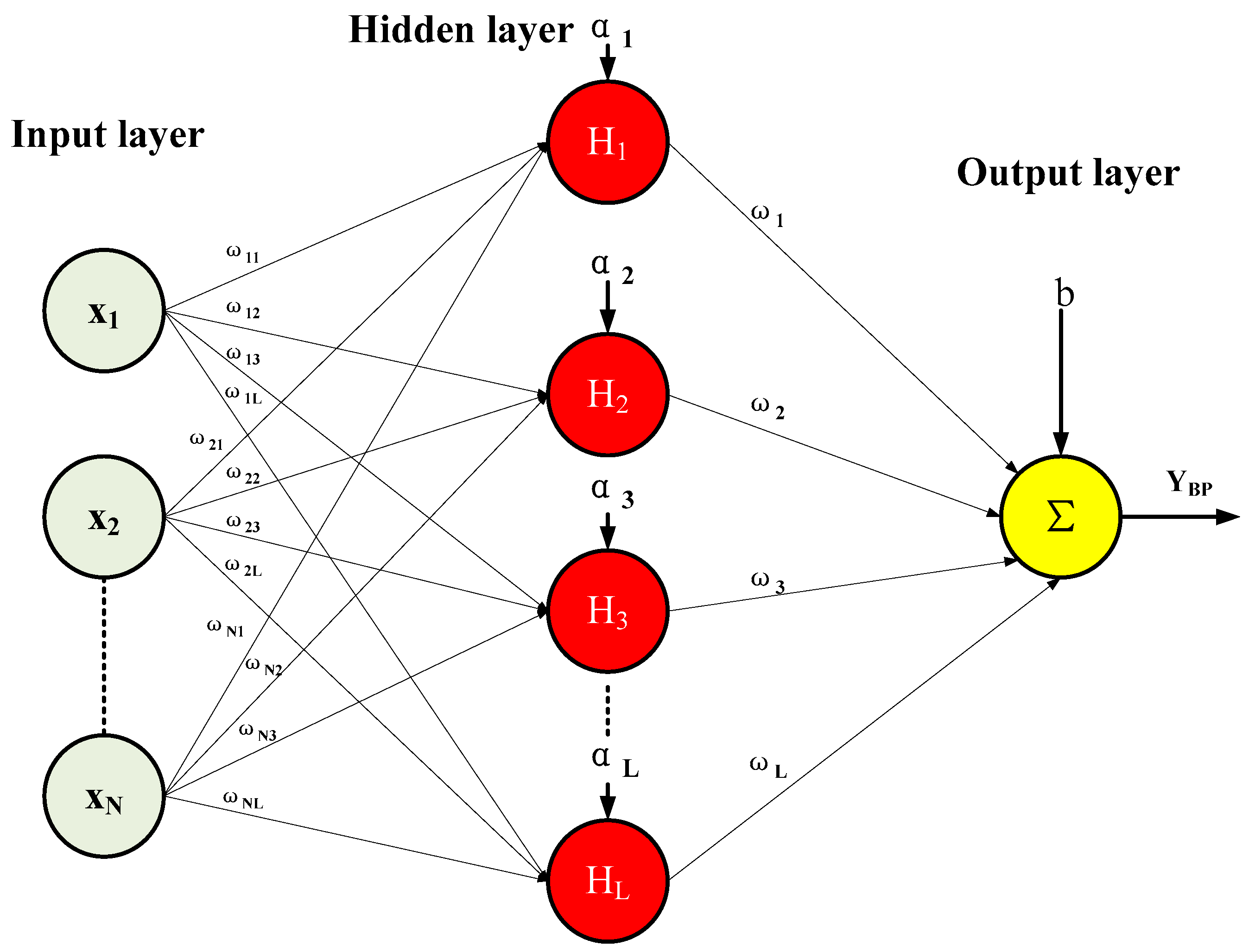
4.1.1. Principles of Mathematics

The BPNN features a multi-layered architecture, as illustrated in Figure 2, comprising input/output and hidden layers [19]. In this structure, computations are iteratively performed through forward propagation from the input layer to the output layer, while the weights and biases are adjusted via backward propagation until the loss function reaches its minimum value.

Figure 2. Typical structure of BPNN.

In Figure 2, the details are outlined as follows:

• First, L represent the number of neurons in the hidden layer and N denote the number of neurons in the input layer, with M signifying the number of neurons in the output layer. The index i for the input layer ranges from 1 to N, while index j spans from 1 to L in the hidden layer;
• Second, the input layer consists of parameters such as the cylinder group volume and gas pressure, gas pipeline length and inner diameter, sea valve inner diameter, blowing duration, sea tank back pressure, ballast water tank level considerations, temperature variations, and the gas volume within the ballast tank; thus, N is set at 10, with X₁ to X_N representing these corresponding inputs;
• Third, H_j(t) denotes the output from each neuron in the jth hidden layer with specific weights assigned between this hidden layer and other layers. The computation for H_j(t) is expressed below:

$${\mathrm{H}}_{\mathrm{j}}\left(\mathrm{t}\right)=\mathrm{f}\left({\displaystyle \sum _{\mathrm{i}=1}^{\mathrm{N}}{\mathsf{\omega }}_{\mathrm{ij}}\cdot {\mathrm{x}}_{\mathrm{i}}\left(\mathrm{t}\right){+\mathsf{\alpha }}_{\mathrm{j}}}\right)$$

(13)

In Equation (13), ω_ij represents the connection weight between the ith neuron in the input layer and the jth neuron in the hidden layer, while α_j denotes the bias associated with the jth hidden-layer neuron. The term x_i(t) refers to the input of the ith neuron layer at time t. Additionally, α_j denotes the bias of the hidden-layer neuron as jth, and f(x) signifies a nonlinear activation function for the hidden layer that facilitates mapping learning capabilities, with common examples including sigmoid, Gaussian, and ReLU functions. Generally, the hyperbolic tangent sigmoid activation function is selected for its S-shaped curve and is expressed as follows:

$$\mathrm{f}\left(\mathrm{x}\right)={\displaystyle \frac{1}{{1+\mathrm{e}}^{-\mathrm{x}}}}$$

(14)

To ensure the effective training of a BPNN, it is essential to appropriately configure the training algorithm. The Levenberg–Marquard method, noted for its rapid convergence rate, is frequently employed [28];

• Fourth, the drainage percentage of the ballast tank is selected as the output result sampled by the output layer; thus, M is assigned a value of 1. The output from the BPNN, denoted as Y_BP(t), can be calculated using the following equation:

$${\mathrm{Y}}_{\mathrm{BP}}\left(\mathrm{t}\right)={\displaystyle \sum _{\mathrm{j}=1}^{\mathrm{L}}\left[{\mathsf{\omega }}_{\mathrm{j}}\cdot {\mathrm{H}}_{\mathrm{j}}\left(\mathrm{t}\right)+\mathrm{b}\right]}$$

(15)

In Equation (15), ω_j represents the weight connecting the jth neuron in the hidden layer to the output-layer neuron, while b denotes the bias of the output layer. The value of L is specified as follows:

$$\mathrm{L}=\sqrt{\mathrm{N}+\mathrm{M}}+\mathrm{a}$$

(16)

In Equation (16), the parameter a is constrained between 1 and 10, which must be validated until the mean square error of the neural network falls below the target training goal [20];

• Fifth, function L (ω, b, X, Y) is defined to quantify the loss between Y_BP(t) and the actual value Y:

$$\mathrm{L}\left(\mathsf{\omega },\mathrm{b},\mathrm{X},\mathrm{Y}\right)={\displaystyle \frac{1}{2}}\cdot {\left(\mathrm{Y}-{\mathrm{Y}}_{\mathrm{BP}}\right)}^2$$

(17)

In Equation (17), Y represents the actual value produced by the BPNN, while YBP denotes the predicted value generated by the BPNN. Through backpropagation, the weights and biases of the various layers are updated via chain iterations as below:

$$\left\{\begin{array}{l}{\mathsf{\omega }}_{\mathrm{ij}}^{\left(\mathrm{k}\right)}={\mathsf{\omega }}_{\mathrm{ij}}^{\left(\mathrm{k}\right)}-\alpha {\displaystyle \frac{\partial \mathrm{L}\left(\mathsf{\omega },\mathrm{b},\mathrm{X},\mathrm{Y}\right)}{\partial {\mathsf{\omega }}_{\mathrm{ij}}^{\left(\mathrm{k}\right)}}}\\ {\mathrm{b}}_{\mathrm{ij}}^{\left(\mathrm{k}\right)}={\mathrm{b}}_{\mathrm{ij}}^{\left(\mathrm{k}\right)}-\alpha {\displaystyle \frac{\partial \mathrm{L}\left(\mathsf{\omega },\mathrm{b},\mathrm{X},\mathrm{Y}\right)}{\partial {\mathrm{b}}_{\mathrm{ij}}^{\left(\mathrm{k}\right)}}}\end{array}\right.$$

(18)

In Equation (18), k represents the number of layers, which is equal to 2, encompassing both the hidden layer and output layer.

4.1.2. Evaluation Indicators

The evaluation metrics employed include the precision percentage (PP%) and relative error percentage (δ), and several standard statistical indicators, such as the sum of square error (E_SSE), mean absolute error (E_MAE), mean absolute percentage error (E_MAP), mean square error (E_MSE), and root mean square error (E_RMSE) [28]:

$$\left\{\begin{array}{l}\mathrm{PP}\%={\displaystyle \sum _{\mathrm{i}=1}^{\mathrm{S}}1\left({\mathrm{X}}_{\mathrm{i}}-0.05\cdot {\mathrm{X}}_{\mathrm{i}}{<\mathrm{Y}}_{\mathrm{i}}{<\mathrm{X}}_{\mathrm{i}}+0.05\cdot {\mathrm{X}}_{\mathrm{i}}\right)}/\mathrm{S}\\ \mathsf{\delta }={\displaystyle \frac{\left|{\mathrm{X}}_{\mathrm{i}}{-\mathrm{Y}}_{\mathrm{i}}\right|}{\left|{\mathrm{X}}_{\mathrm{i}}\right|}}\cdot 100\%\\ {\mathrm{E}}_{\mathrm{SSE}}={\displaystyle \sum _{\mathrm{i}=1}^{\mathrm{S}}{\left({\mathrm{X}}_{\mathrm{i}}{-\mathrm{Y}}_{\mathrm{i}}\right)}^2}\\ {\mathrm{E}}_{\mathrm{MAE}}={\displaystyle \sum _{\mathrm{i}=1}^{\mathrm{S}}\left|\left({\mathrm{X}}_{\mathrm{i}}{-\mathrm{Y}}_{\mathrm{i}}\right)\right|}/\mathrm{S}\\ {\mathrm{E}}_{\mathrm{MAP}}={\displaystyle \sum _{\mathrm{i}=1}^{\mathrm{S}}\left|\left({\mathrm{X}}_{\mathrm{i}}{-\mathrm{Y}}_{\mathrm{i}}\right)/{\mathrm{X}}_{\mathrm{i}}\right|}/\mathrm{S}\\ {\mathrm{E}}_{\mathrm{MSE}}={\displaystyle \sum _{\mathrm{i}=1}^{\mathrm{S}}{\left({\mathrm{X}}_{\mathrm{i}}{-\mathrm{Y}}_{\mathrm{i}}\right)}^2}/\mathrm{S}\\ {\mathrm{E}}_{\mathrm{RMSE}}=\sqrt{{\displaystyle \sum _{\mathrm{i}=1}^{\mathrm{S}}{\left({\mathrm{X}}_{\mathrm{i}}{-\mathrm{Y}}_{\mathrm{i}}\right)}^2}/\mathrm{S}}\end{array}\right.$$

(19)

In Equation (19), S denotes the number of datasets; X_i represents the actual value, with its average as $\overline{{\mathrm{X}}_{\mathrm{i}}}$; and Y_i indicates the prediction value, and its average is $\overline{{\mathrm{Y}}_{\mathrm{i}}}$. Below is a concise description of each indicator:

• The precision percentage (PP%) employs an indicator function that equals 1 if the condition in parentheses is met; otherwise, it is 0;
• The relative error (δ) measures the percentage ratio of the absolute difference between X_i and Y_i for the absolute value of X_i;
• The square sum of errors (E_SSE) computes the total errors between Y_i and X_i. While easy to calculate, it can be affected by outliers, distorting the overall error distribution;
• The mean absolute error (E_MAE) calculates the average absolute differences between Y_i and X_i. It remains stable against outliers but may miss some distribution details;
• The mean absolute percentage error (E_MAP) evaluates the prediction error percentage between Y_i and X_i. Like E_MAE, it is unaffected by anomalies but can become unstable when the actual values are zero;
• The mean square error (E_MSE) reflects the average derived from E_SSE. Although more robust than other metrics, it remains sensitive to outliers that might overshadow smaller errors;
• The root mean square error (E_RMSE), being the square root of E_MSE, enables the measurement of prediction errors across different dimensions on a common scale. Similar to E_MSE, E_RMSE also shows sensitivity toward larger discrepancies.

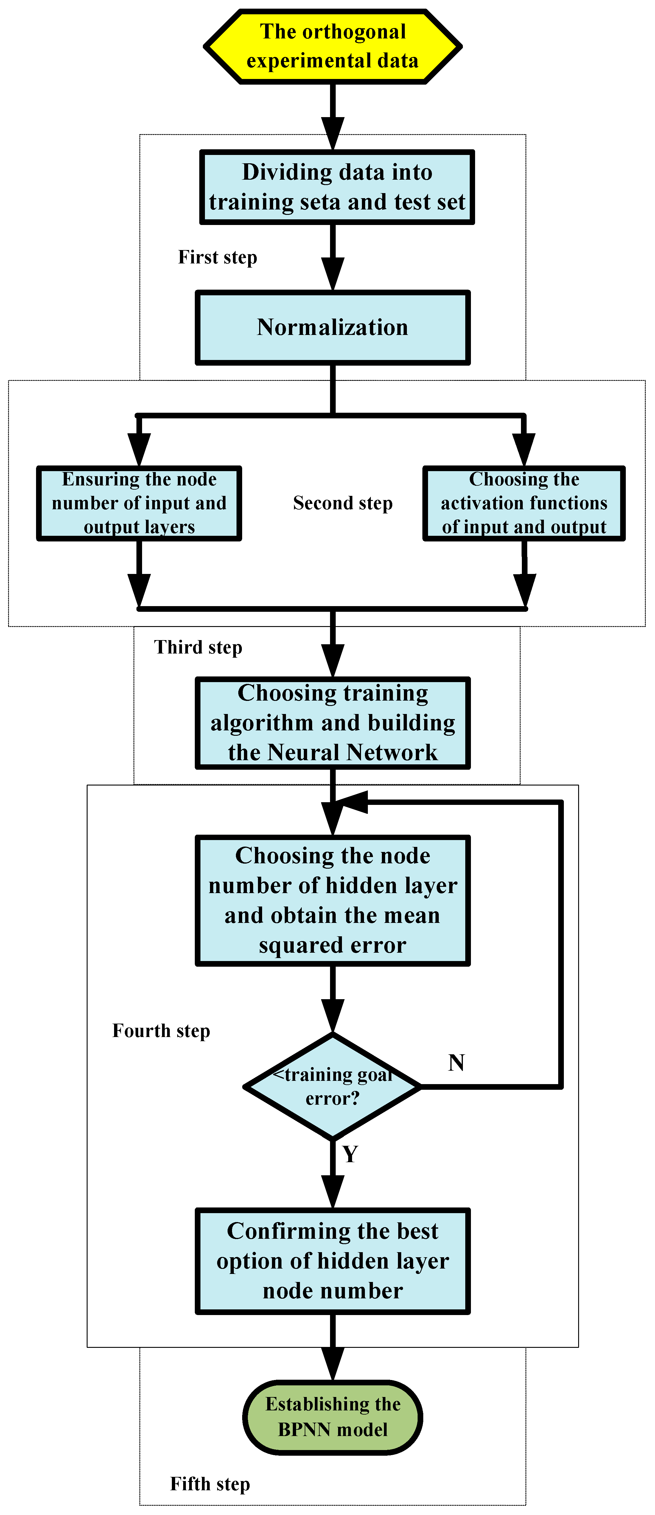
4.1.3. Proposed Algorithm

This paper introduces a BPNN algorithm comprising five components, with the procedures detailed in Figure 3.

Figure 3. The proposed algorithm of BPNN.

• First, the orthogonal experimental data were collected and divided into training and testing sets. Subsequently, normalization was performed to accurately capture the inherent characteristics of the data while eliminating scale restrictions [29];
• Second, the number of input and output nodes was determined based on the criteria outlined in Section 4.1.1, with the activation functions of both the input and output layers set to tansy and purlin by default;
• Third, the Levenberg–Marquard algorithm was selected for training, establishing a neural network with parameters including 1000 training epochs, a 0.01 learning rate, and a 10⁻⁵ minimal training goal error;
• Fourth, the number of hidden layers was chosen according to Equation (13), utilizing the specified training in the prepared neural network to calculate the mean square error. If this value falls below the specified training goal error, then the corresponding number of hidden layer nodes is confirmed as optimal;
• Fifth, confirming the BPNN model is achieved by incorporating all the relevant data and information above before commencing predictions.

4.2. Computation Analysis

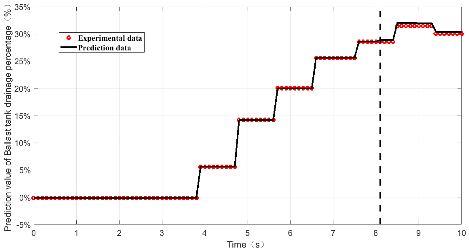
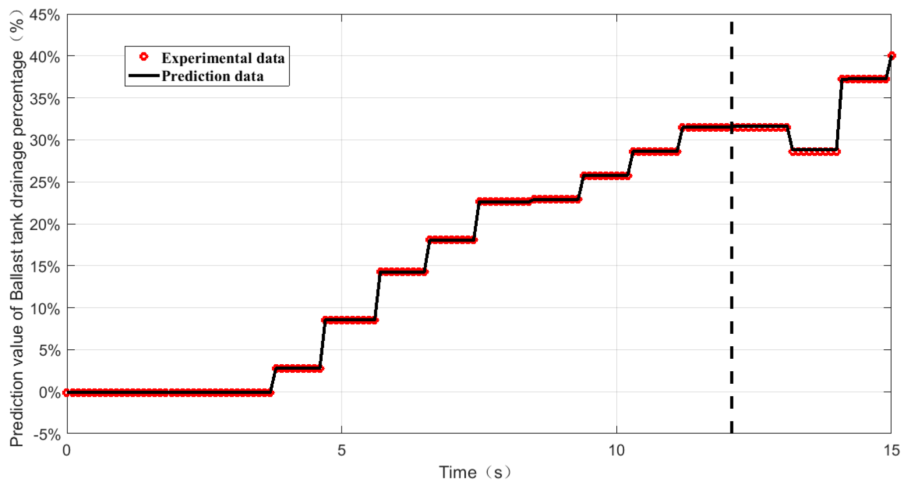
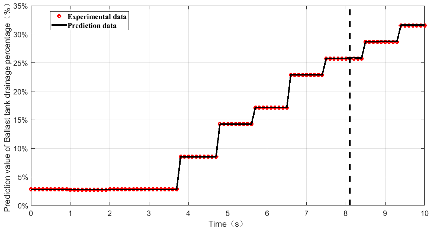
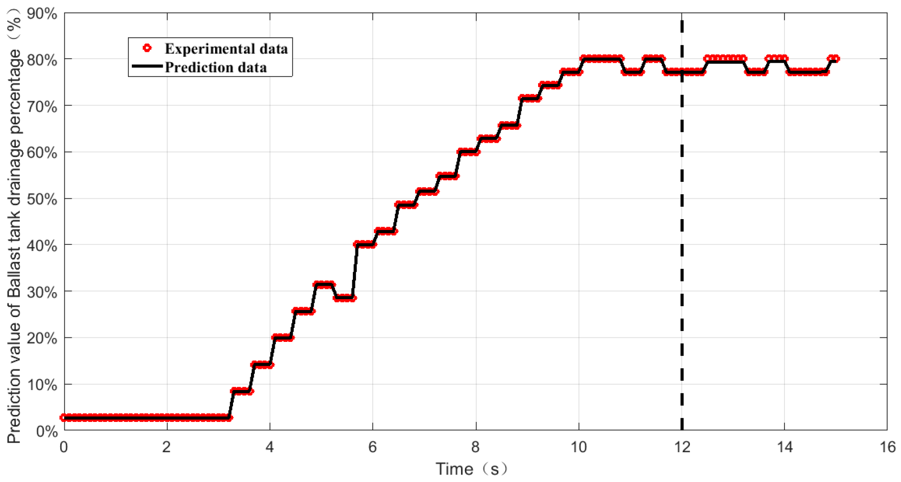
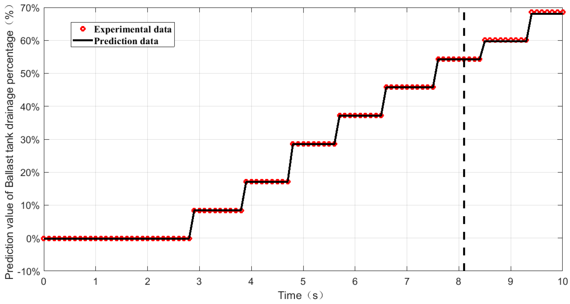
4.2.1. Evaluation of Working Conditions

The training set comprised 10 input parameters: blowing duration (s), gas pressure in the cylinder group (MPa), volume of the cylinder group (L), liquid level within the ballast tank (cm), length of the gas supply pipeline (m), inner diameter of the gas supply pipeline (mm), inner diameter of the sea valve (mm), gas pressure inside the ballast tank (MPa), temperature within the ballast tank (MPa), and back pressure from the sea tank (MPa). Additionally, there was one output variable: the drainage percentage from the ballast tank, which is dimensionless. The predicted values derived from this training set were compared to the actual measurements, as illustrated in Figure 4, Figure 5, Figure 6, Figure 7, Figure 8, Figure 9, Figure 10, Figure 11, Figure 12, Figure 13, Figure 14, Figure 15, Figure 16, Figure 17, Figure 18, Figure 19, Figure 20 and Figure 21, while the dashed line shows the boundary between the training set and test set, with the training set on the left and the test set on the right:

Figure 4. Evaluation of working condition 1.

Figure 5. Evaluation of working condition 2.

Figure 6. Evaluation of working condition 3.

Figure 7. Evaluation of working condition 4.

Figure 8. Evaluation of working condition 5.

Figure 9. Evaluation of working condition 6.

Figure 10. Evaluation of working condition 7.

Figure 11. Evaluation of working condition 8.

Figure 12. Evaluation of working condition 9.

Figure 13. Evaluation of working condition 10.

Figure 14. Evaluation of working condition 11.

Figure 15. Evaluation of working condition 12.

Figure 16. Evaluation of working condition 13.

Figure 17. Evaluation of working condition 14.

Figure 18. Evaluation of working condition 15.

Figure 19. Evaluation of working condition 16.

Figure 20. Evaluation of working condition 17.

Figure 21. Evaluation of working condition 18.

In Figure 4, Figure 5, Figure 6, Figure 7, Figure 8, Figure 9, Figure 10, Figure 11, Figure 12, Figure 13, Figure 14, Figure 15, Figure 16, Figure 17, Figure 18, Figure 19, Figure 20 and Figure 21, different line symbols were used to identify the prediction values and actual values, in which the black solid line represents the prediction values, while the red dots represent the actual values. It can be inferred that the BPNN can predict the test set data well after training, and the prediction and actual values are consistent.

According to the specific evaluation indicators in 4.1.2, a comparative study was carried out, and the indicators were analyzed, as shown in Table 6 below:

Table 6. Evaluation indicators of 18working conditions.

Index	Evaluation Indicators	Data	Remarks
Working condition 1	Sum of Square Errors, ESSE	1.8906∙10−12	Fit between predicted and actual values
	Mean Absolute Error, EMAE	4.4939∙10−7	Average absolute difference between predicted and actual values
	Mean Absolute Percentage Error, EMAP	0.00055853	Error across datasets with varying magnitudes
	Mean Square Error, EMSE	2.7008∙10−13	Mean square error of prediction discrepancies
	Root Mean Square Error, ERMSE	5.1969∙10−7	The square root of the mean square differences between predicted and actual values
Working condition 2	Sum of Square Errors, ESSE	0.00012022	Fit between predicted and actual values
	Mean Absolute Error, EMAE	0.001514	Average absolute difference between predicted and actual values
	Mean Absolute Percentage Error, EMAP	0.0036052	Error across datasets with varying magnitudes
	Mean Square Error, EMSE	2.4043∙10−6	Mean square error of prediction discrepancies
	Root Mean Square Error, ERMSE	0.0015506	The square root of the mean square differences between predicted and actual values
Working condition 3	Sum of Square Errors, ESSE	0.00016132	Fit between predicted and actual values
	Mean Absolute Error, EMAE	0.0011673	Average absolute difference between the predicted and actual values
	Mean Absolute Percentage Error, EMAP	0.0029131	Error across datasets with varying magnitudes
	Mean Square Error, EMSE	1.9436∙10−6	Mean square error of prediction discrepancies
	Root Mean Square Error, ERMSE	0.0013941	The square root of the mean square differences between predicted and actual values
Working condition 4	Sum of Square Errors, ESSE	0.0061557	Fit between predicted and actual values
	Mean Absolute Error, EMAE	0.0096929	Average absolute difference between the predicted values and actual values
	Mean Absolute Percentage Error, EMAP	0.023948	Error across datasets with varying magnitudes
	Mean Square Error, EMSE	0.00012311	Mean square error of prediction discrepancies
	Root Mean Square Error, ERMSE	0.011096	The square root of the mean square differences between predicted and actual values
Working condition 5	Sum of Square Errors, ESSE	0.001105	Fit between predicted and actual values
	Mean Absolute Error, EMAE	0.0046973	Average absolute difference between the predicted values and actual values
	Mean Absolute Percentage Error, EMAP	0.0059697	Error across datasets with varying magnitudes
	Mean Square Error, EMSE	2.21∙10−5	Mean square error of prediction discrepancies
	Root Mean Square Error, ERMSE	0.004701	The square root of the mean square differences between predicted and actual values
Working condition 6	Sum of Square Errors, ESSE	0.0064002	Fit between predicted and actual values
	Mean Absolute Error, EMAE	0.0080078	Average absolute difference between the predicted and actual values
	Mean Absolute Percentage Error, EMAP	0.028729	Error across datasets with varying magnitudes
	Mean Square Error, EMSE	9.1432∙10−5	Mean square error of prediction discrepancies
	Root Mean Square Error, ERMSE	0.009562	The square root of the mean square differences between predicted and actual values
Working condition 7	Sum of Square Errors, ESSE	5.5945∙10−5	Fit between predicted and actual values
	Mean Absolute Error, EMAE	0.00081209	Average absolute difference between the predicted and actual values
	Mean Absolute Percentage Error, EMAP	0.004057	Error across datasets with varying magnitudes
	Mean Square Error, EMSE	1.1189∙10−6	Mean square error of prediction discrepancies
	Root Mean Square Error, ERMSE	0.0010578	The square root of the mean square differences between predicted and actual values
Working condition 8	Sum of Square Errors, ESSE	0.00635	Fit between predicted and actual values
	Mean Absolute Error, EMAE	0.0095017	Average absolute difference between the predicted and actual values
	Mean Absolute Percentage Error, EMAP	0.011281	Error across datasets with varying magnitudes
	Mean Square Error, EMSE	0.00010583	Mean square error of prediction discrepancies
	Root Mean Square Error, ERMSE	0.010288	The square root of the mean square differences between predicted and actual values
Working condition 9	Sum of Square Errors, ESSE	0.00030943	Fit between predicted and actual values
	Mean Absolute Error, EMAE	0.0024449	Average absolute difference between the predicted and actual values
	Mean Absolute Percentage Error, EMAP	0.0061119	Error across datasets with varying magnitudes
	Mean Square Error, EMSE	6.1887∙10−6	Mean square error of prediction discrepancies
	Root Mean Square Error, ERMSE	0.0024877	The square root of the mean square differences between predicted and actual values
Working condition 10	Sum of Square Errors, ESSE	7.5391∙10−5	Fit between predicted and actual values
	Mean Absolute Error, EMAE	0.0011243	Average absolute difference between the predicted and actual values
	Mean Absolute Percentage Error, EMAP	0.0028055	Error across datasets with varying magnitudes
	Mean Square Error, EMSE	1.5078∙10−6	Mean square error of prediction discrepancies
	Root Mean Square Error, ERMSE	0.0012279	The square root of the mean square differences between predicted and actual values
Working condition 11	Sum of Square Errors, ESSE	8.0629∙10−5	Fit between predicted and actual values
	Mean Absolute Error, EMAE	0.0016049	Average absolute difference between the predicted and actual values
	Mean Absolute Percentage Error, EMAP	0.0064002	Error across datasets with varying magnitudes
	Mean Square Error, EMSE	5.0393∙10−6	Mean square error of prediction discrepancies
	Root Mean Square Error, ERMSE	0.0022448	The square root of the mean square differences between predicted and actual values
Working condition 12	Sum of Square Errors, ESSE	0.00011633	Fit between predicted and actual values
	Mean Absolute Error, EMAE	0.0011062	Average absolute difference between the predicted and actual values
	Mean Absolute Percentage Error, EMAP	0.0066337	Error across datasets with varying magnitudes
	Mean Square Error, EMSE	1.2245∙10−6	Mean square error of prediction discrepancies
	Root Mean Square Error, ERMSE	0.0011066	The square root of the mean square differences between predicted and actual values
Working condition 13	Sum of Square Errors, ESSE	0.00021467	Fit between predicted and actual values
	Mean Absolute Error, EMAE	0.0012303	Average absolute difference between the predicted and actual values
	Mean Absolute Percentage Error, EMAP	0.0015655	Error across datasets with varying magnitudes
	Mean Square Error, EMSE	2.9009∙10−6	Mean square error of prediction discrepancies
	Root Mean Square Error, ERMSE	0.0017032	The square root of the mean square differences between predicted and actual values
Working condition 14	Sum of Square Errors, ESSE	0.00014928	Fit between predicted and actual values
	Mean Absolute Error, EMAE	0.0011504	Average absolute difference between the predicted and actual values
	Mean Absolute Percentage Error, EMAP	0.010992	Error across datasets with varying magnitudes
	Mean Square Error, EMSE	1.3951∙10−6	Mean square error of prediction discrepancies
	Root Mean Square Error, ERMSE	0.0011812	The square root of the mean square differences between predicted and actual values
Working condition 15	Sum of Square Errors, ESSE	0.00017113	Fit between predicted and actual values
	Mean Absolute Error, EMAE	0.0015861	Average absolute difference between the predicted and actual values
	Mean Absolute Percentage Error, EMAP	0.0023651	Error across datasets with varying magnitudes
	Mean Square Error, EMSE	2.5542∙10−6	Mean square error of prediction discrepancies
	Root Mean Square Error, ERMSE	0.0015982	The square root of the mean square differences between predicted and actual values
Working condition 16	Sum of Square Errors, ESSE	0.00094847	Fit between predicted and actual values
	Mean Absolute Error, EMAE	0.0072352	Average absolute difference between the predicted and actual values
	Mean Absolute Percentage Error, EMAP	0.017463	Error across datasets with varying magnitudes
	Mean Square Error, EMSE	5.2693∙10−5	Mean square error of prediction discrepancies
	Root Mean Square Error, ERMSE	0.007259	The square root of the mean square differences between predicted and actual values
Working condition 17	Sum of Square Errors, ESSE	0.00049875	Fit between predicted and actual values
	Mean Absolute Error, EMAE	0.002734	Average absolute difference between the predicted and actual values
	Mean Absolute Percentage Error, EMAP	0.0077481	Error across datasets with varying magnitudes
	Mean Square Error, EMSE	9.975∙10−6	Mean square error of prediction discrepancies
	Root Mean Square Error, ERMSE	0.0031583	The square root of the mean square differences between predicted and actual values
Working condition 18	Sum of Square Errors, ESSE	0.0043433	Fit between predicted and actual values
	Mean Absolute Error, EMAE	0.0063359	Average absolute difference between the predicted and actual values
	Mean Absolute Percentage Error, EMAP	0.012839	Error across datasets with varying magnitudes
	Mean Square Error, EMSE	5.6407∙10−5	Mean square error of prediction discrepancies
	Root Mean Square Error, ERMSE	0.0075104	The square root of the mean square differences between predicted and actual values

As detailed in the table above, the metrics E_SSE, E_MAE, E_MAP, E_MSE, and E_RMSE for the orthogonal experimental working conditions 1–18 demonstrate the fidelity of the BPNN predictions. Among these 18 working conditions, the maximum values recorded were as follows: E_SSE was 0.011281, E_MAE was 0.0096929, E_MAP was 0.028729, E_MSE was 0.011281, and E_RMSE was 0.011096. All remained within a threshold of 0.03, thereby proving that the BPNN could deliver high-quality prediction results [26].

4.2.2. Relative Error and Prediction Accuracy Analysis

Referring to Equation (17), the relative error (δ) and the prediction accuracy (PP%) of the ballast tank drainage percentage under the orthogonal experimental conditions were analyzed. Using 3% as the threshold [19], the prediction accuracy for all 18 conditions was evaluated through enumeration, as presented in Table 7:

Table 7. Maximal relative errors and precision accuracy of 18 working conditions.

Index	Maximal Value of δ	Prediction Accuracy PP%
Working condition 1	0.00%	100%
Working condition 2	0.57%	100%
Working condition 3	0.17%	100%
Working condition 4	0.14%	100%
Working condition 5	0.77%	100%
Working condition 6	0.18%	100%
Working condition 7	0.26%	100%
Working condition 8	0.63%	100%
Working condition 9	0.06%	100%
Working condition 10	0.28%	100%
Working condition 11	1.57%	100%
Working condition 12	0.17%	100%
Working condition 13	0.41%	100%
Working condition 14	0.04%	100%
Working condition 15	0.05%	100%
Working condition 16	0.30%	100%
Working condition 17	0.50%	100%
Working condition 18	0.85%	100%

The histograms of relative error for the 18 orthogonal experimental conditions above are shown in Figure 22, Figure 23, Figure 24, Figure 25, Figure 26, Figure 27, Figure 28, Figure 29, Figure 30, Figure 31, Figure 32, Figure 33, Figure 34, Figure 35, Figure 36, Figure 37, Figure 38 and Figure 39, where the horizontal axis represents the sample number, and the vertical axis denotes the relative error.

Figure 22. Prediction precision percentages of working condition 1.

Figure 23. Prediction precision percentages of working condition 2.

Figure 24. Prediction precision percentages of working condition 3.

Figure 25. Prediction precision percentages of working condition 4.

Figure 26. Prediction precision percentages of working condition 5.

Figure 27. Prediction precision percentages of working condition 6.

Figure 28. Prediction precision percentages of working condition 7.

Figure 29. Prediction precision percentages of working condition 8.

Figure 30. Prediction precision percentages of working condition 9.

Figure 31. Prediction precision percentages of working condition 10.

Figure 32. Prediction precision percentages of working condition 11.

Figure 33. Prediction precision percentages of working condition 12.

Figure 34. Prediction precision percentages of working condition 13.

Figure 35. Prediction precision percentages of working condition 14.

Figure 36. Prediction precision percentages of working condition 15.

Figure 37. Prediction precision percentages of working condition 16.

Figure 38. Prediction precision percentages of working condition 17.

Figure 39. Prediction precision percentages of working condition 18.

4.2.3. Correlation Analysis of Individual Influencing Factors

The Pearson correlation calculation method quantitatively reflects the positive or negative correlations between individual factors and experimental data, serving as an effective counterpart to extreme variance analysis. Pearson’s linear correlation coefficient (R) was computed as follows:

$$\mathrm{R}={\displaystyle \sum _{\mathrm{i}=1}^{\mathrm{S}}\left({\mathrm{X}}_{\mathrm{i}}-\overline{{\mathrm{X}}_{\mathrm{i}}}\right)\cdot \left({\mathrm{Y}}_{\mathrm{i}}-\overline{{\mathrm{Y}}_{\mathrm{i}}}\right)}/\sqrt{{\displaystyle \sum _{\mathrm{i}=1}^{\mathrm{S}}{\left({\mathrm{X}}_{\mathrm{i}}-\overline{{\mathrm{X}}_{\mathrm{i}}}\right)}^2\cdot {\displaystyle \sum _{\mathrm{i}=1}^{\mathrm{S}}{\left({\mathrm{Y}}_{\mathrm{i}}-\overline{{\mathrm{Y}}_{\mathrm{i}}}\right)}^2}}}$$

(20)

In Equation (20), Pearson’s linear correlation coefficient R showed a value ranging from −1 to 1, where the interval of 0–1 could be subdivided as follows: 0.0–0.2 was considered very weak or no correlation, 0.2–0.4 indicated a weak correlation, 0.4–0.6 represented a moderate correlation, 0.6–0.8 signified a strong correlation, and 0.8–1.0 denoted a very strong correlation. This classification was similarly applied to the −1–0 interval.

The correlation between the individual factors and the ballast tank drainage percentage was verified for the 18 orthogonal experimental conditions [30]. The parameters selected for generating Pearson’s correlation analysis heat map included blowing duration (s), the cylinder group with gas pressure (MPa) and volume (L), the ballast tank liquid level (cm), gas supply pipeline with length (m) and inner diameter (mm), the sea valve inner diameter (mm), the ballast tank with gas pressure (MPa) and temperature (MPa), the sea tank back pressure (MPa), and the ballast tank drainage percentage (dimensionless), as illustrated in Figure 40.

Figure 40. Pearson analysis heat map.

The logical relationship between each factor and the blowing process provided supplementary insights to the conclusions drawn from the orthogonal experiments in Section 3.1 and Section 3.2:

• First, the blowing duration exhibited a correlation coefficient of 0.6535, indicating a strong positive correlation. Theoretically, a longer gas supply duration resulted in a greater amount of water being expelled [31];
• Second, the sea tank back pressure had a value of 0.8105, reflecting an extremely strong positive correlation. This suggests that the ballast tank drainage was closely related to the outboard back pressure through a complex relationship. Specifically, the variations in back pressure influenced the pressure changes during blowing within the ballast tank [12,32]. Additionally, back pressure affected the dynamic balance between gas and water, as well as the corresponding blowing efficiency [2,31]. Finally, it impacted energy consumption and system efficiency during blowing operations [12,32];
• Third, the volume of the gas cylinder group was associated with a correlation coefficient of 0.3587, indicating a weak positive correlation. According to the aerodynamic computation theories, there exists a direct relationship between gas consumption and ballast tank drainage [32];
• Fourth, the gas pressure within the cylinder group registered at 0.5569, indicating a moderately strong positive correlation and suggesting that higher gas pressure significantly affected blowing effectiveness [13];
• Fifth, the inner diameter of the gas supply pipeline showed a value of 0.02499, and this represents a very weak positive correlation. Theoretically speaking, a larger inner diameter would have increased the gas supply efficiency over time, which would facilitate the quicker establishment of gas cushions at the top of the ballast tank, thereby improving the overall blowing performance [12]. However, due to size constraints on the flow dynamics caused by only having pipe diameters available at 6 (mm), 8 (mm), and 10 (mm), with lengths limited to just 0.3 (m);
• Sixth, the length of the gas supply pipeline was −0.3741, indicating a medium-strength negative correlation. This finding confirms that shorter pipeline lengths yielded better blowing effects under constant conditions and further validates the advantage of short-circuit blowing over conventional methods [12];
• Seventh, the internal diameter of the sea valve was measured to be 0.5373, demonstrating a moderately positive correlation. It indicates that increasing the sea valve flowing area enhanced the drainage rates per unit of time while improving the blowing efficiency [13].

4.2.4. Comparison Analysis with Existing Results

Referring to Table 1, existing results from short-circuit experiments in refs. [2,10,11], as well as those related to gas jet blowing in refs. [8,9], were analyzed and compared with this study, as presented in Table 8:

Table 8. Comparison of existing results and this study.

Index of Literature	Relative Error	Research Objects
Ref. [2]	0.53–39.17%	Peak pressure of ballast tank, which was directly related to drainage percentage
Refs. [10,11]	8%	The flowing rate of the high-pressure gas cylinder group, which was closely related to the drainage percentage
Ref. [8]	<5%	Drainage percentage by gas jet blowing-off, which is a similar method to short-circuit blowing
Ref. [9]	<10%	Drainage percentage by gas jet blowing-off, which is a similar method to short-circuit blowing
This study	0.00–1.57%	Drainage percentage of ballast tank during short-circuit blowing

• In ref. [2], Table 8 indicates that the relative errors of peak pressure in ballast tanks, directly associated with the drainage percentage, ranged from 0.53% to 39.17%, significantly exceeding the results shown in Table 7 of Section 4.2.2;
• In refs. [10,11], the small-scale short-circuit experimental test bench focused on the flow rate of high-pressure gas cylinder groups closely linked to the ballast tank drainage percentage. Their relative error was found to be 8%, considerably larger than the maximum relative error reported in Table 7 of Section 4.2.2;
• In refs. [8,9], using a gas jet blowing-off method similar to short-circuit blowing resulted in a relative error for the drainage percentage below 5% and individually below 10%. However, these values still exceeded those presented in Table 7 of Section 4.2.2;
• From this comparative analysis, it could be inferred that the BPNN method demonstrates significantly higher prediction accuracy than traditional numerical modeling; furthermore, no statistical correlation studies were identified between the manipulation factors and the blowing process in Section 3.1, Section 3.2 and Section 4.2.3.

5. Conclusions

In this paper, a model test bench designed for submersible high-pressure gas proportional short-circuit blowing was employed to perform L₁₈ (3⁷) orthogonal experiments encompassing multiple factors at various levels. Furthermore, the training and prediction results derived from the 18 orthogonal experiments were subjected to analysis using a BPNN and Pearson correlation. The key conclusions are summarized below:

• First, an extreme variance method was utilized to analyze the data from the orthogonal experiments, identifying the optimal combination of several factors: blowing duration (accounting for 39.16%), back pressure (accounting for 33.35%), gas blowing group pressure (accounting for 10.94%), and sea valve flow area (9.02%). Among these variables, blowing duration proved to be the most sensitive factor, with an F-ratio of 3.27;
• Second, a BPNN was implemented for both training and prediction based on the orthogonal experimental data. The findings indicate that the BPNN’s robust nonlinear fitting capability effectively predicted high-pressure gas short-circuit blowing. The statistical evaluation metrics ranged from 10⁻¹ to 10⁻¹², the relative errors remained within a threshold of 3%, and the prediction accuracy achieved up to 100%. This validates the BPNN as a credible AI-based predictive approach for submersible short-circuit blowing;
• Third, Pearson correlation analysis was conducted on the BPNN’s training set data to explore the relationship between the individual factors and outcomes. The results reveal positive correlations among the following: blowing duration (with a correlation coefficient of 0.6535), sea tank back pressure (0.8105), gas cylinder group pressure (with a correlation coefficient of 0.5569), and internal diameter of the sea valve (0.5373). In contrast, a negative correlation (-0.3741) with the gas supply pipeline length indicates the better efficiency of short-circuit blowing compared to conventional methods.

Building on the previously discussed conclusions, a series of recommendations for engineering design and operational practices related to submersible high-pressure gas short-circuit blowing are presented below:

• First, concerning blowing techniques, short-circuit blowing exhibits superior efficiency compared to conventional methods due to its reduced length of gas supply pipelines;
• Second, in terms of engineering design, several manipulation factors, including the increased volume and pressure of the cylinder group, as well as the enlarged flow area of the sea valve, have a positive impact on blowing performance. Additionally, it is crucial to establish appropriate specifications for the gas supply pipeline, including its inner diameter and length;
• Third, concerning operations, it is of vital importance to ensure that the optimal duration of blowing corresponds to the variations in the outboard back pressure during the operation process.

In summary, this study introduces a robust predictive methodology for submersible short-circuit blowing, providing valuable recommendations for engineering design and operational protocols. This encompasses the advantages of the short-circuit blowing technique, the optimal working condition configurations, and operational strategies. These findings may also offer effective solutions for similar scenarios involving submersibles or submarines, including submersible hovering maneuvers and medium-pressure gas discharges.

With the rapid advancements in the IoT and Virtual Reality (VR) technologies, future investigations could establish a digital twin model of the submersible short-circuit blowing process to assess more extreme operational conditions or perform a feature analysis of real vessels within virtual environments, thereby revealing further principles governing submersible safety.

References

- Zhang, J.H.; Hu, K.; Liu, C.B. Numerical simulation on compressed gas blowing ballast tank of submarine. J. Ship Mech. 2015, 19, 363–368. (In Chinese) [Google Scholar] [CrossRef]
- Yi, Q.; Lin, B.; Zhang, W.; Qian, Y.; Zou, W.; Zhang, K. Simulation and experimental verification of main ballast tank blowing based on short circuit blowing model. Chin. J. Ship Res. 2022, 17, 246–252. [Google Scholar] [CrossRef]
- Wang, X.; Wang, X.; Zhang, Z.; Feng, D. Experiment and Mathematics Model of High Pressure Air Blowing. Chin. J. Ship Res. 2014, 9, 80–86. [Google Scholar] [CrossRef]
- Zhang, J.; Huang, H.; Liu, G.; Hu, K. Numerical simulation of blowing characteristics of submarine main ballast tanks using VOF model. J. Ordnance Equip. Eng. 2022, 43, 234–239. [Google Scholar] [CrossRef]
- Zhang, J.; Hu, K.; Huang, H.; Wei, J. Analysis of the influence of 90° elbow on the pressure loss along the submarine high pressure gas pipe. Ship Sci. Technol. 2020, 42, 93–97. [Google Scholar]
- Jin, T.; Liu, H.; Wang, J.; Yang, F. Emergency recovery of submarine with flooded compartment. J. Ship Mech. 2010, 14, 34–43. [Google Scholar]
- Wilgenhof, J.D.; Giménez JJ, C.; Peláez, J.G. Performance of the main ballast tank blowing system. In Proceedings of the Undersea Defense Technology Conference 2011, London, UK, 7–9 June 2011. [Google Scholar]
- Sheng, Y.; Yu, J.; Cheng, D.; Gong, S. Theoretical analysis and experimental validation on gas jet blowing-off process of submarine emergency. J. Beijing Univ. Aeronaut. Astronaut. 2009, 35, 411–416. [Google Scholar]
- Yang, S.; Yu, J.Z.; Cheng, D. Numerical simulation and experimental validation on gas jet blowing-off process of submarine emergency. J. Beijing Univ. Aeronaut. Astronaut. 2010, 36, 227–230. [Google Scholar] [CrossRef]
- Liu, H.; Pu, J.; Li, Q.; Wu, X. The experiment research of submarine high-pressure air blowing off main ballast tanks. J. Harbin Eng. Univ. 2013, 34, 34–39. [Google Scholar] [CrossRef]
- Liu, H.; Li, Q.X.; Wu, X.J.; Li, Z. The establishing of pipe flow model and experimental analysis on submarine high pressure air blowing system. Ship Sci. Technol. 2015, 37, 52–55. [Google Scholar] [CrossRef]
- Liu, H.; Pu, J.; Jin, T. Research on system model of high pressure air blowing submarine’s main ballast tanks. Ship Sci. Technol. 2010, 32, 26–30. [Google Scholar] [CrossRef]
- Yi, Q.; Lin, B.; Zhang, W.; Chen, S.; Zou, W.; Zhang, K. CFD simulation and experimental verification of blowing process of main ballast tank. J. Ship Mech. 2023, 27, 218–226. [Google Scholar]
- Yi, Q.; Lin, B.; Zhang, W. Analysis of the blowing process of high pressure air from the bottom into the main ballast tank. Ship Sci. Technol. 2020, 42, 60–63. [Google Scholar] [CrossRef]
- Wang, C.; Fang, Y.; Su, G.; Tian, W.; Qiu, S. A High Temperature and High Flowing Rate Gas Flow Heat Transfer Experimental Device and Experimental Method. International Patent Application No. 201910377151.1, 10 July 2020. (In Chinese). [Google Scholar]
- Yang, X.; Ren, Z. Design and Analyses of Orthogonal Test with Null Ratio Factor. J. Biomath. 2006, 2, 291–296. [Google Scholar]
- Wu, W.; Xu, Z.; Teng, K.; Yan, S.; Zhang, L. Process Parameters Optimization for 2AL2 Aluminum Alloy Laser Cutting Based on Orthogonal Experiment and BP Neural Network. Mach. Tool Hydraul. 2018, 46, 13–17. [Google Scholar] [CrossRef]
- Assani, N.; Matic, P.; Kastelan, N.; Cavka, I.R. A review of artificial neural networks application in Maritime Industry. IEEE Access 2023, 11, 139823–139848. [Google Scholar] [CrossRef]
- Zhang, Y.; Hu, Q.W.; Li, H.L.; Li, J.Y.; Liu, T.C.; Chen, Y.T.; Ai, M.Y.; Dong, J.Y. A Back Propagation Neural Network-Based Radiometric Correction Method (BPNNRCM) for UAV Multispectral Image. IEEE J. Sel. Top. Appl. Earth Obs. Remote Sens. 2022, 16, 112–125. [Google Scholar] [CrossRef]
- Zhang, H.; Han, D.; Guo, C. Modeling of the principal dimensions of large vessels based on a BPNN trained by an improved PSO. J. Harbin Eng. Univ. 2012, 33, 806–810. [Google Scholar] [CrossRef]
- Pān, J.; Shàn, P. Fundamentals of Gas Dynamics, 1st ed.; National Defense Industry Press: Beijing, China, 2017; p. 164. (In Chinese) [Google Scholar]
- Liu, M. Variance Analysis of Orthogonal Experimental Design. Master’s Thesis, Northeast Forestry University, Harbin, China, April 2011. [Google Scholar]
- Yang, K. Design and Key Technology Research on High Pressure Pneumatic Blowing Valve with Differential Pressure Control. Master’s Thesis, Wuhan Institute of Technology, Wuhan, China, 2015. [Google Scholar]
- Hao, H. Times Series Forecasting Based on Feed-Forward Neural Networks. Master’s Thesis, Nanjing University, Nanjing, China, 2021. [Google Scholar]
- Panda, J.P. Machine learning for naval architecture, ocean and marine engineering. J. Mar. Sci. Technol. 2023, 28, 1–26. [Google Scholar] [CrossRef]
- Huang, L.; Pena, B.; Liu, Y.; Anderlini, E. Machine learning in sustainable ship design and operation: A review. Ocean. Eng. 2022, 266, 112907. [Google Scholar] [CrossRef]
- Shi, Y. Ship Structure Optimization Based on PSO-BP Neural Network; Dalian Maritime University: Dalian, China, 2015. [Google Scholar]
- Shao, M.; Yu, Y. Optimization of Gas-liquid Two-phase Flow Liquid Hold-up Prediction Model with BP Neural Network Based on Genetic Algorithm. J. Xi’an Shiyou Univ. (Nat. Sci. Ed.) 2019, 34, 44–49. [Google Scholar] [CrossRef]
- Wang, Y. Analysis of Normalization for Deep Neural Networks. Master’s Thesis, Nanjing University of Posts and Telecommunications, Nanjing, China, 2019. [Google Scholar]
- Barnett, I.; Mukherjee, R.; Lin, X. The generalized higher criticism for testing SNP-Set Effects in Genetic Association studies. J. Am. Stat. Assoc. 2017, 112, 64–76. [Google Scholar] [CrossRef] [PubMed]
- Font, R.; Garcia-Peláez, J. On a submarine hovering system based on blowing and venting of ballast tanks. Ocean. Eng. 2013, 72, 441–447. [Google Scholar] [CrossRef]
- Chen, L.; Yang, P.; Li, S.; Liu, K.; Wang, K.; Zhou, X. Online modeling and prediction of maritime autonomous surface ship maneuvering motion under ocean waves. Ocean. Eng. 2023, 276, 114183. [Google Scholar] [CrossRef]