
A Method to Improve Underwater Positioning Reference Based on Topological Distribution Constraints of Multi-INSs


Abstract
1. Introduction
2. Single-Axis Rotating Inertial Navigation Systems
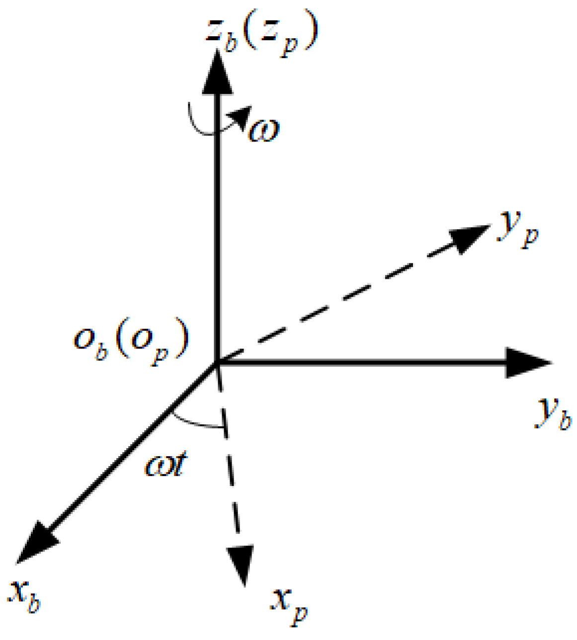
2.1. Definition of an SRINS Coordinate System
2.2. Error Model of the SRINS
2.3. State Equations of the SRINS
3. The Model of Flexible Arm
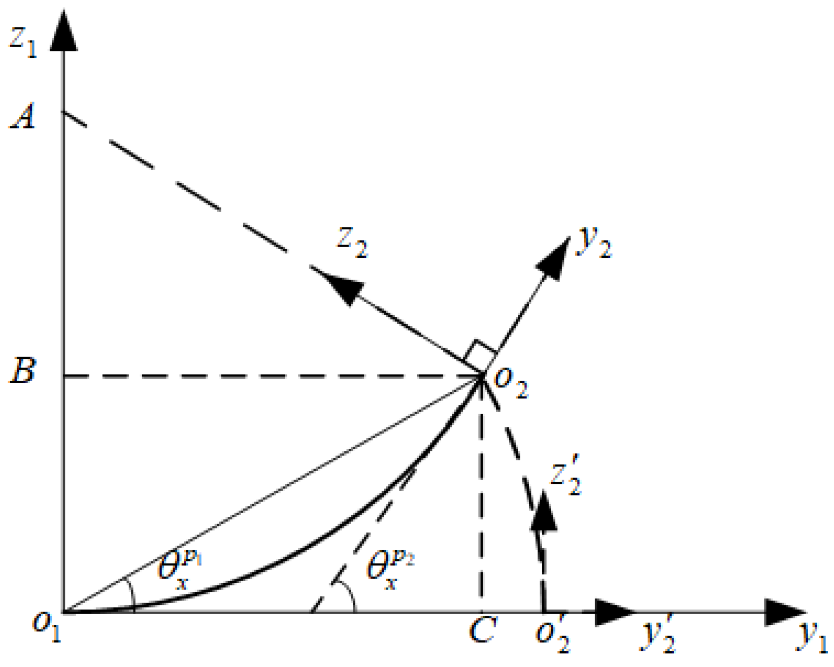
3.1. Deformation Angle Modeling
3.2. Relationship Between Lever Arms and Deformation Angles
4. Establishing the Data Fusion Kalman Filter Equations
4.1. State Equation
4.2. Measurement Equation
4.3. Calculation Process
| Algorithm 1: Three SRINSs Data Fusion algorithm. |
Input: Gyroscope and accelerometer increments measured by the three sets of SRINSs , , . Output: Comprehensive position result after data fusion. For different SRINS i, the inertial navigation calculation process is as follows: 1: 2: 3: 4: After the three sets of SRINSs have completed their calculations, they enter the Kalman filter process, where the state variables are: , 5: 6: 7: 8: 9: 10: 11: 12: Prediction, Compensation, and Position Output Process: 13: 14: 15: , where represents the position error estimation variance of SRINSi. |
5. Experimental Analysis
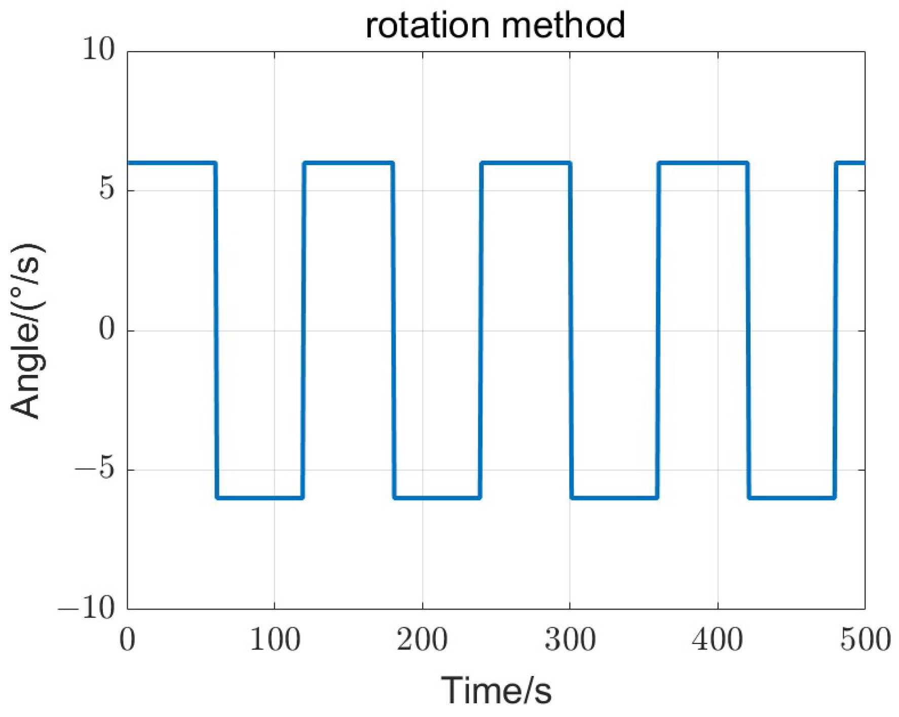
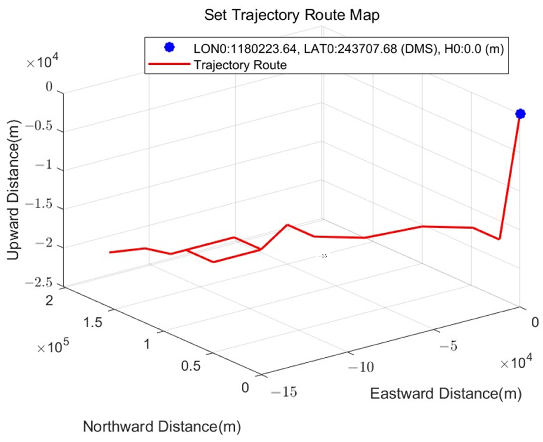
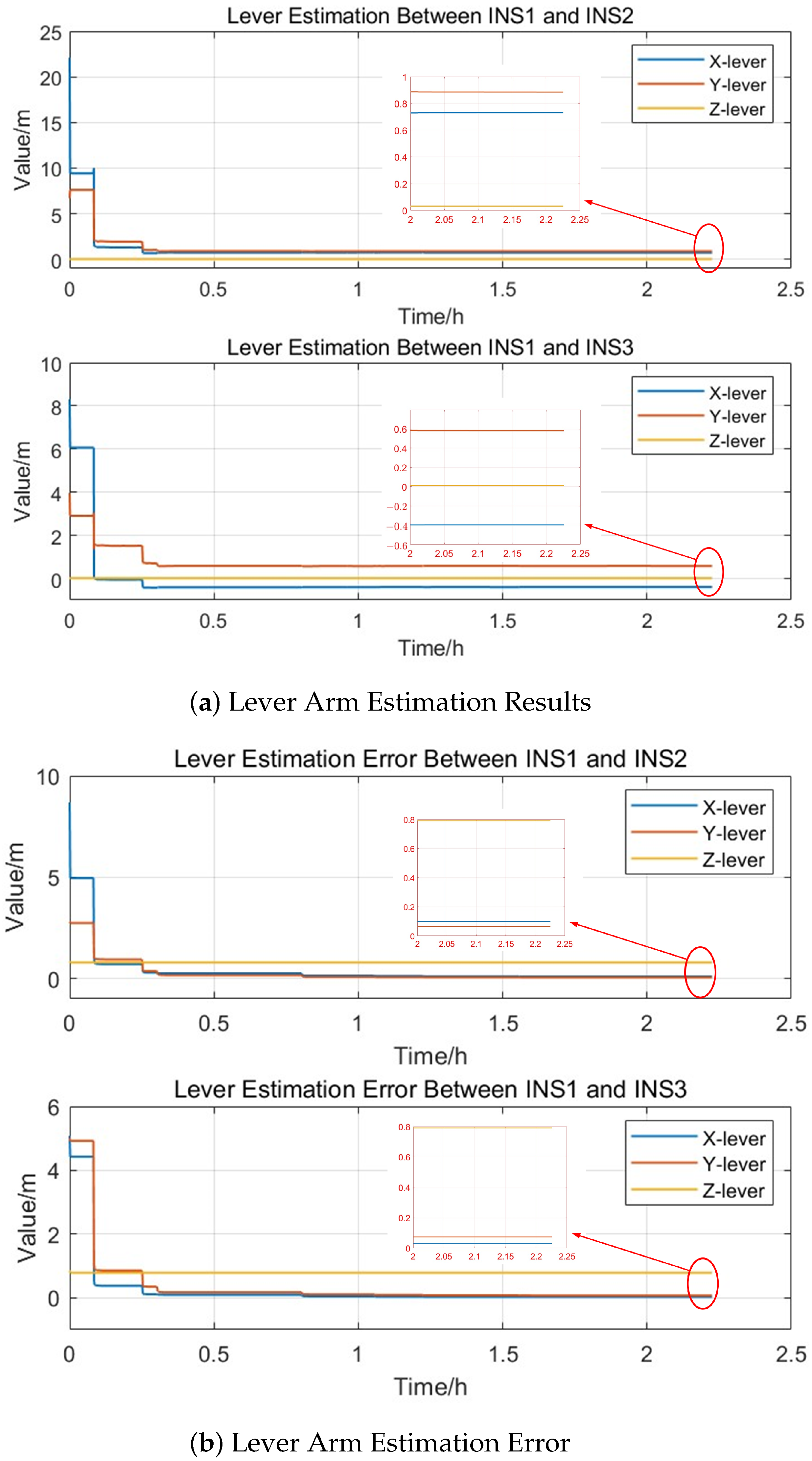
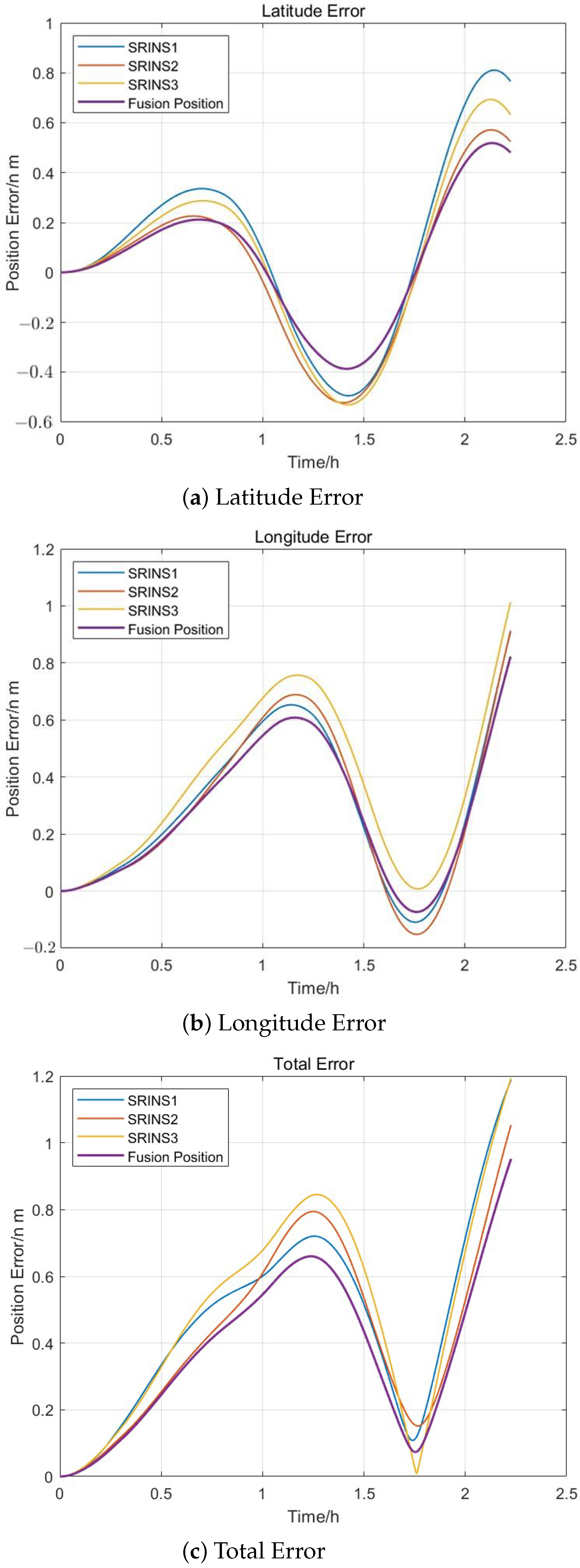
5.1. Simulation Experiment
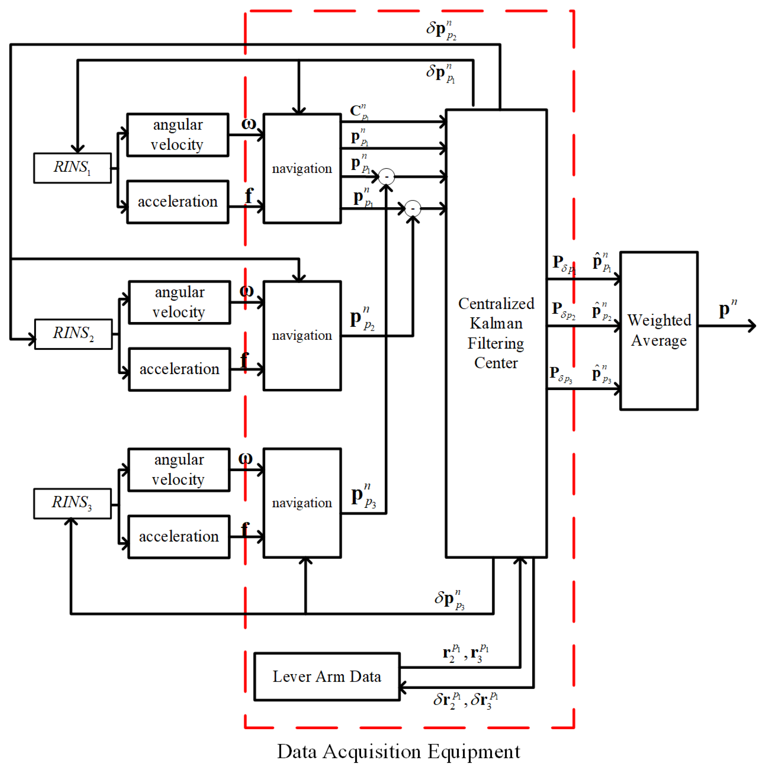
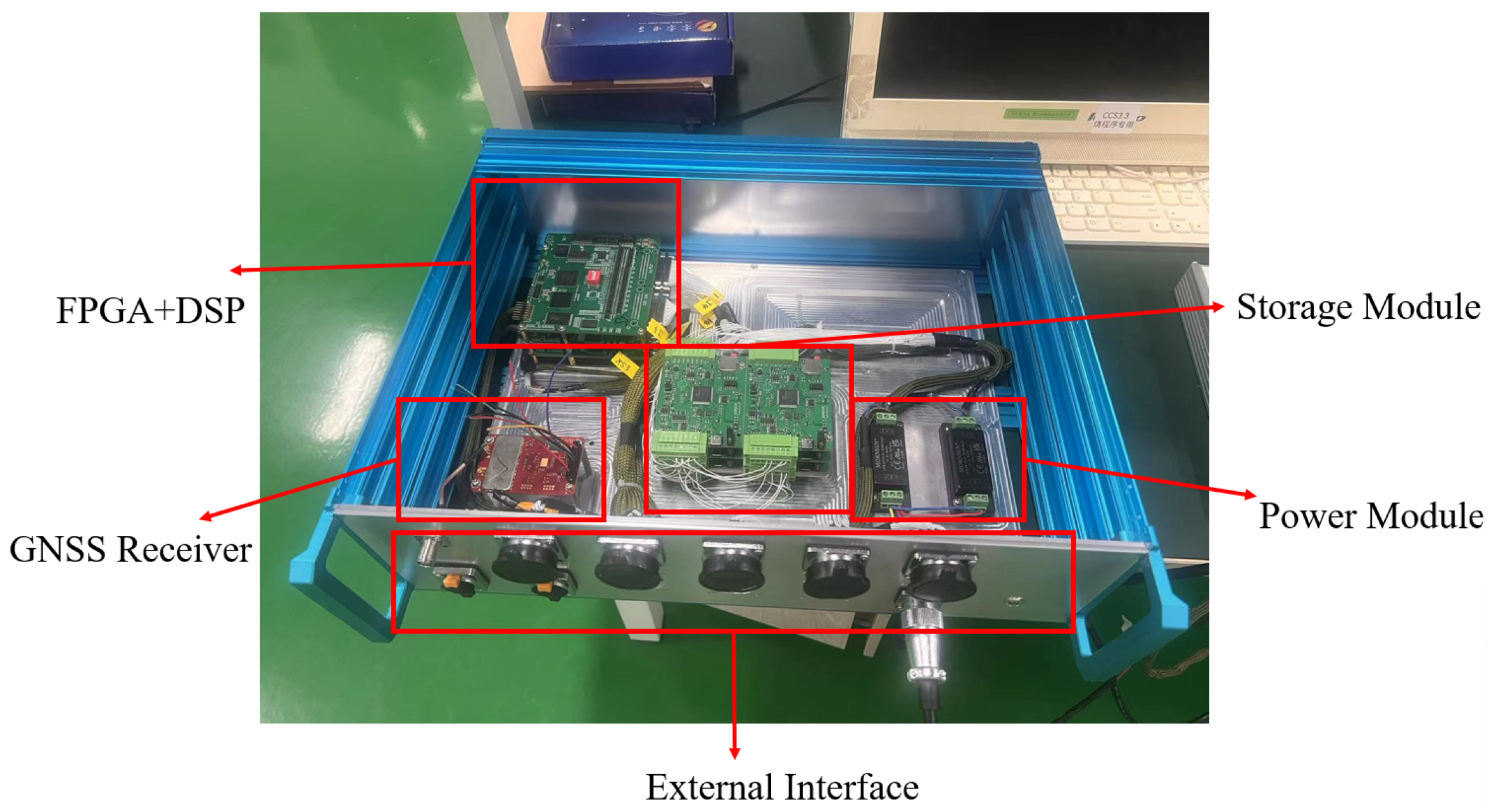
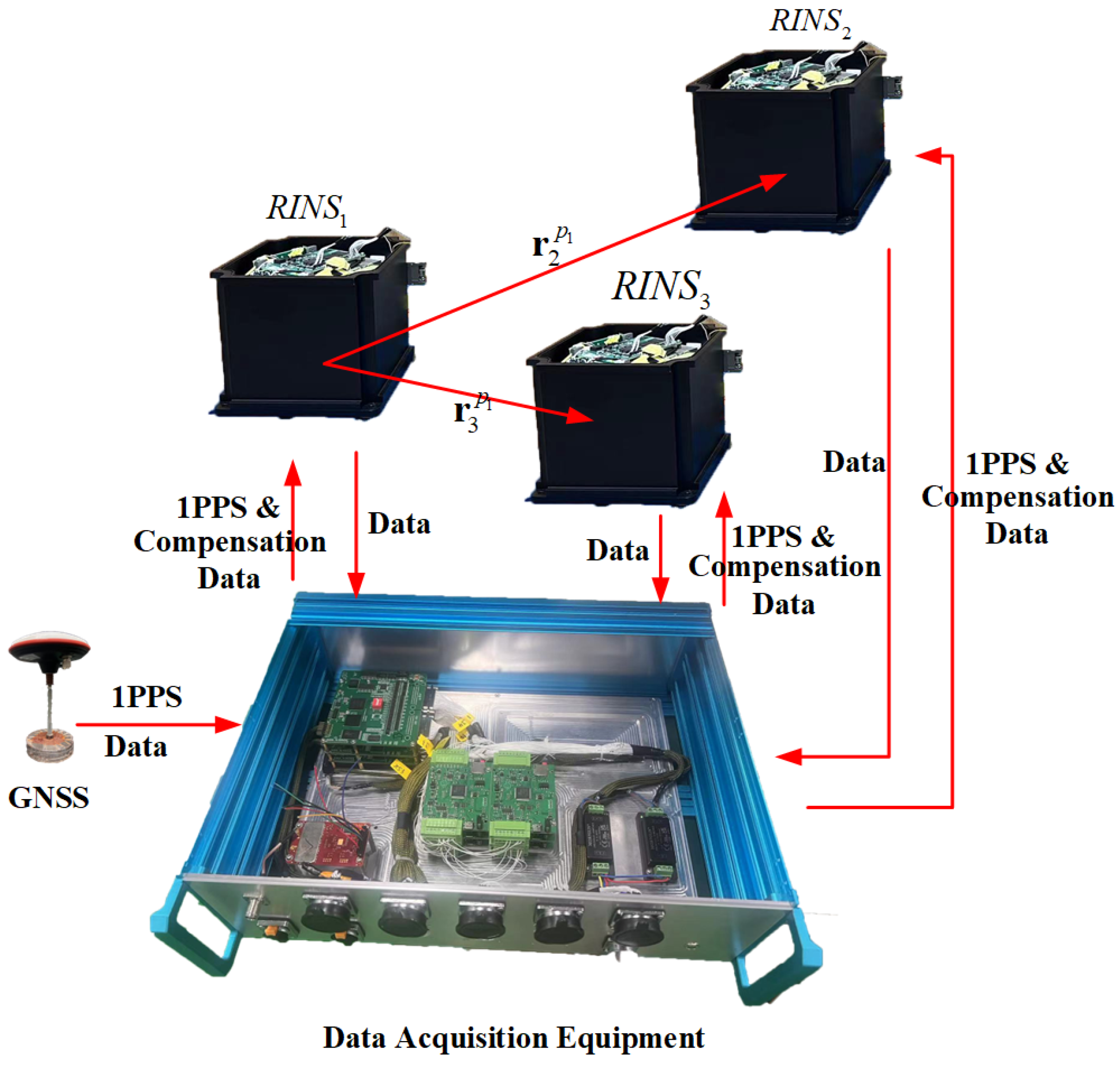
5.2. Data Acquisition Equipment
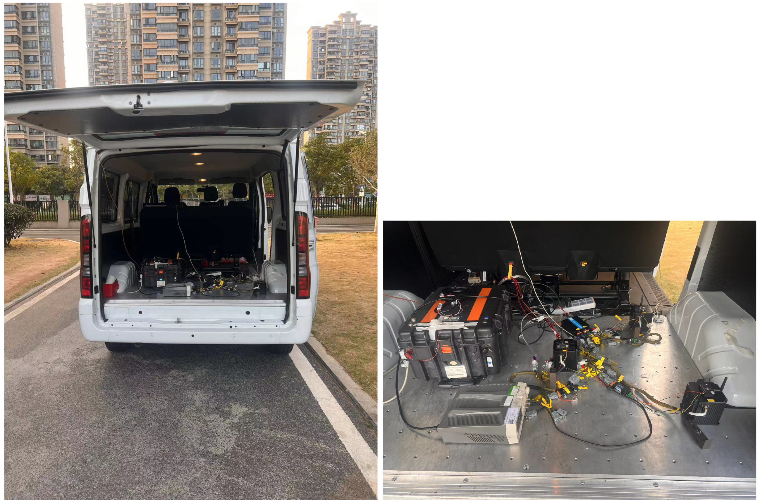
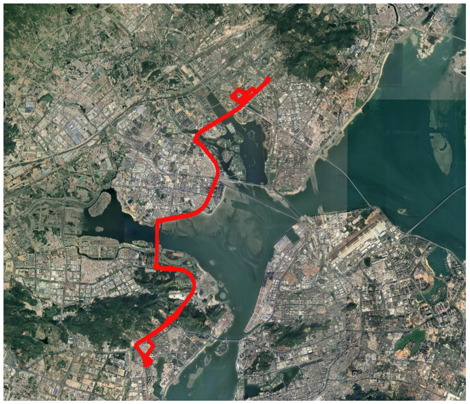
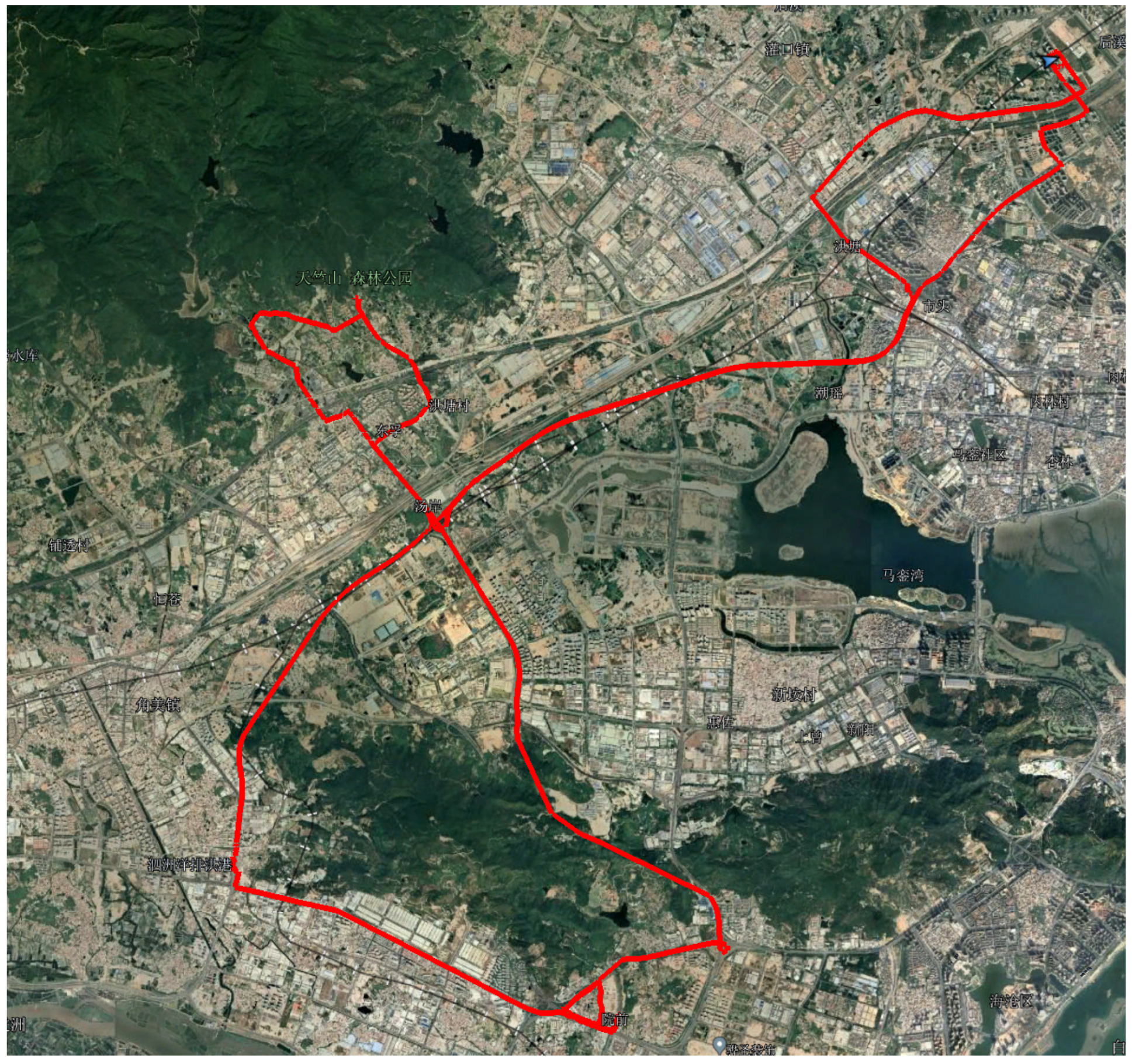
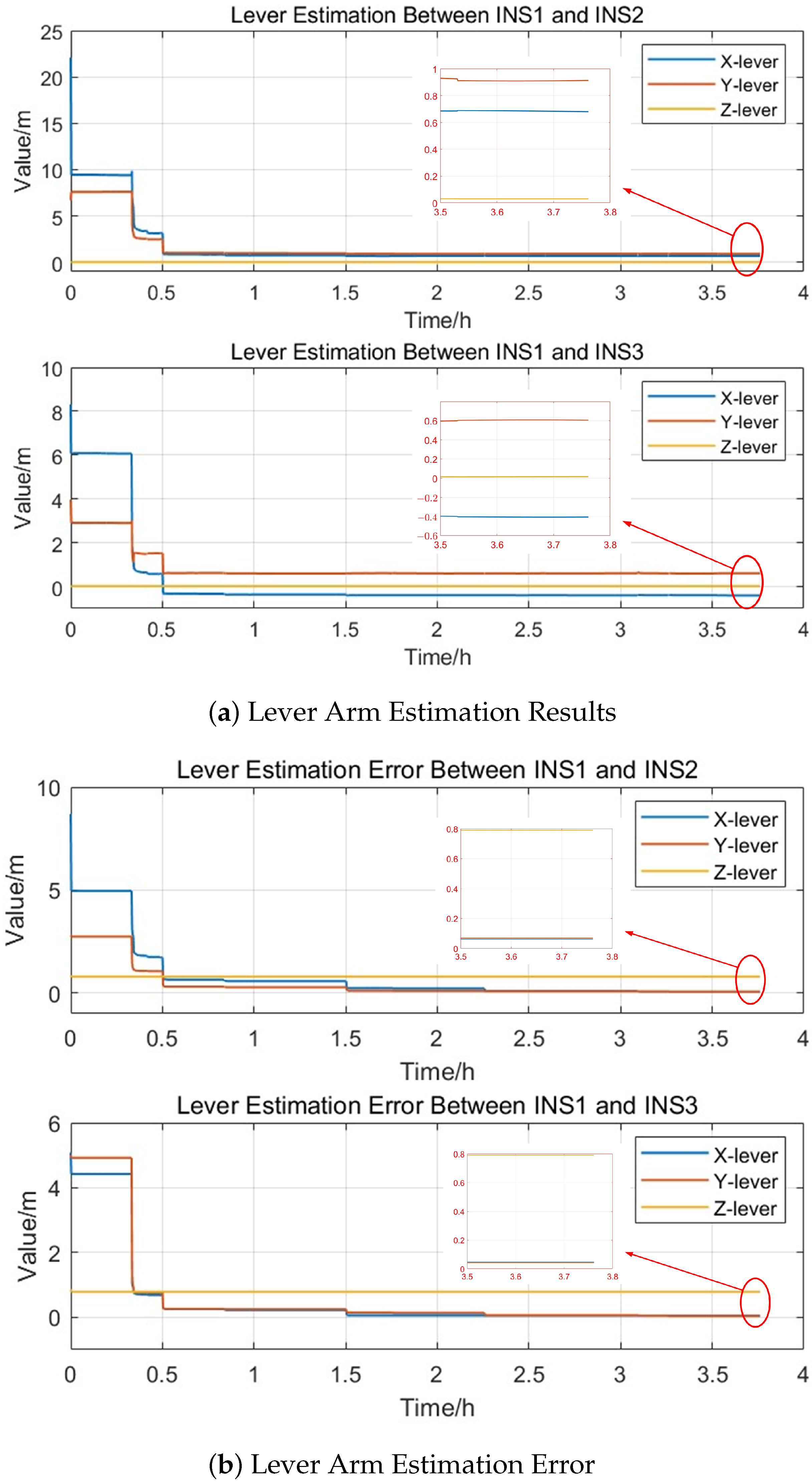
5.3. Sports Vehicles Test Analysis
6. Conclusions
Author Contributions
Funding
Institutional Review Board Statement
Informed Consent Statement
Data Availability Statement
Conflicts of Interest
References
- Zhai, X.; Ren, Y.; Wang, L.; Zhu, T.; He, Y.; Lv, B. A Review of Redundant Inertial Navigation Technology. In Proceedings of the 2021 International Conference on Computer, Control and Robotics (ICCCR), Shanghai, China, 8–10 January 2021; pp. 272–278. [Google Scholar]
- Tazartes, D. An historical perspective on inertial navigation systems. In Proceedings of the 2014 International Symposium on Inertial Sensors and Systems (INERTIAL), Laguna Beach, CA, USA, 25–26 February 2014; pp. 1–5. [Google Scholar]
- Wang, Z.; Cheng, X.; Du, J. Thermal modeling and calibration method in complex temperature field for single-axis rotational inertial navigation system. Sensors 2020, 20, 384. [Google Scholar] [CrossRef] [PubMed]
- Li, K.; Chen, Y.; Wang, L. Online self-calibration research of single-axis rotational inertial navigation system. Measurement 2018, 129, 633–641. [Google Scholar] [CrossRef]
- Nie, B.; Chen, G.; Luo, X.; Liu, B. Error Mechanism and Self-Calibration of Single-Axis Rotational Inertial Navigation System. Math. Probl. Eng. 2019, 2019, 8912341. [Google Scholar] [CrossRef]
- Sun, C.; Li, K. A positioning accuracy improvement method by couple RINSs information fusion. IEEE Sens. J. 2021, 21, 19351–19361. [Google Scholar] [CrossRef]
- Kuznetsov, I.M.; Veremeenko, K.K.; Zharkov, M.V.; Pronkin, A.N. Moving object SINS transfer alignment time synchronization parameters estimation. J. Phys. Conf. Ser. 2021, 1925, 012025. [Google Scholar] [CrossRef]
- Yang, J.; Wang, X.; Ji, X.; Hu, X.; Nie, G. A new high-accuracy transfer alignment method for distributed INS on moving base. Measurement 2024, 227, 114302. [Google Scholar] [CrossRef]
- Li, J.; Qu, C. A novel transfer alignment method of array POS based on lever-arm estimation. IEEE Trans. Instrum. Meas. 2022, 71, 1–11. [Google Scholar] [CrossRef]
- Wang, Q.; Yang, C.S.; Wu, S.E.; Wang, Y.X. Lever arm compensation of autonomous underwater vehicle for fast transfer alignment. Comput. Mater. Contin. 2019, 59, 105–118. [Google Scholar] [CrossRef]
- Wu, Q.; Li, K. An inertial device biases on-line monitoring method in the applications of two rotational inertial navigation systems redundant configuration. Mech. Syst. Signal Process. 2019, 120, 133–149. [Google Scholar] [CrossRef]
- Wu, Q.; Li, K.; Liang, W. An improved calibration and compensation method for lever-arm errors between two rotational inertial navigation systems. In Proceedings of the 2019 IEEE International Conference on Mechatronics and Automation (ICMA), Tianjin, China, 4–7 August 2019; pp. 2457–2462. [Google Scholar]
- Wu, Q.; Li, K.; Liu, J. The asynchronous gimbal-rotation-based calibration method for lever-arm errors of two rotational inertial navigation systems. IEEE Access 2018, 7, 4653–4663. [Google Scholar] [CrossRef]
- Sahu, N.; Babu, P.; Kumar, A.; Bahl, R. A Novel Algorithm for Optimal Placement of Multiple Inertial Sensors to Improve the Sensing Accuracy. IEEE Trans. Signal Process. 2020, 68, 142–154. [Google Scholar] [CrossRef]
- Hua, M.; Li, K.; Lv, Y.; Wu, Q. A dynamic calibration method of installation misalignment angles between two inertial navigation systems. Sensors 2018, 18, 2947. [Google Scholar] [CrossRef]
- Wang, M.; Wang, L.; Han, H. Research on improving heading and attitudes accuracy by online calibration of errors based on multi-RINSs joint rotation modulation. IEEE Sens. J. 2022, 22, 4503–4513. [Google Scholar] [CrossRef]
- Qiu, T.; Zhao, Y.; Ben, Y.; Hou, L.; Wang, K.; Zhang, R. Multiple Sets of High-Precision Inertial Navigation Information Fusion Strategy Based on Confidence Analysis. In Proceedings of the 2023 IEEE International Conference on Mechatronics and Automation (ICMA), Harbin, China, 6–9 August 2023; pp. 181–188. [Google Scholar]
- Liang, W.; Li, K. A dynamic calibration and compensation method for the asynchronous time between two inertial navigation systems. IEEE Sens. J. 2021, 21, 10091–10101. [Google Scholar] [CrossRef]
- Wang, L.; Wu, W.; Wei, G.; Pan, X.; Lian, J. Navigation information fusion in a redundant marine rotational inertial navigation system configuration. J. Navig. 2018, 71, 1531–1552. [Google Scholar] [CrossRef]
- Wang, L.; Wu, W.; Wei, G.; Lian, J.; Yu, R. A polar-region-adaptable systematic bias collaborative measurement method for shipboard redundant rotational inertial navigation systems. Meas. Sci. Technol. 2018, 29, 055106. [Google Scholar] [CrossRef]
- Li, X.; Qin, S.; Wang, X.; Tan, W.; Zheng, J.; Zhao, Y. Multi Inertial Navigation System Fusion Method Considering Ship Deformation. In Proceedings of the 2023 30th Saint Petersburg International Conference on Integrated Navigation Systems (ICINS), Saint Petersburg, Russia, 29–31 May 2023; pp. 1–10. [Google Scholar]
- Cai, Q.; Yang, G.; Song, N.; Yin, H.; Liu, Y. Analysis and calibration of the gyro bias caused by geomagnetic field in a dual-axis rotational inertial navigation system. Meas. Sci. Technol. 2016, 27, 105001. [Google Scholar] [CrossRef]
- Cai, Q.; Yang, G.; Song, N.; Wang, L.; Yin, H.; Liu, Y. Online calibration of the geographic-frame-equivalent gyro bias in dual-axis RINS. IEEE Trans. Instrum. Meas. 2018, 67, 1609–1616. [Google Scholar] [CrossRef]
- Wang, L.; Wu, W.; Lian, J.; Kong, X. Redundant RINS Information Fusion with Application to Shipborne Transfer Alignment. In Proceedings of the 2018 21st International Conference on Information Fusion (FUSION), Cambridge, UK, 10–13 July 2018; pp. 2246–2253. [Google Scholar]
- Chen, X.; Ma, Z.; Yang, P. Integrated modeling of motion decoupling and flexure deformation of carrier in transfer alignment. Mech. Syst. Signal Process. 2021, 159, 107690. [Google Scholar] [CrossRef]


| Parameter Error Items | Element | Parameter Settings |
|---|---|---|
| Gyroscope | Constant Drift | /h |
| Random Walk Coefficient | ||
| Scale Factor Error | 10 ppm | |
| Accelerometer | Constant Bias | |
| Random Walk Coefficient | ||
| Scale Factor Error | 10 ppm | |
| Initial Attitude Setting | Pitch Angle | |
| Roll Angle | ||
| Heading Angle | ||
| Initial Velocity Setting | Eastward Velocity | 0 m/s |
| Northward Velocity | 0 m/s | |
| Upward Velocity | 0 m/s | |
| Lever between SRINS1 and SRINS2 | X-direction | 0.255 m |
| Y-direction | 0.375 m | |
| Z-direction | 0 m | |
| Lever between SRINS1 and SRINS3 | X-direction | 0.409 m |
| Y-direction | 0.030 m | |
| Z-direction | 0.800 m | |
| Deformation Angle | Correlation Time | 100 s |
| Standard Deviation | ||
| Initial Position Setting | Latitude | |
| Longitude | ||
| Altitude | 0 m | |
| Other Settings | Simulation Duration | 8 h |
| Simulation Step Size | 20 ms |
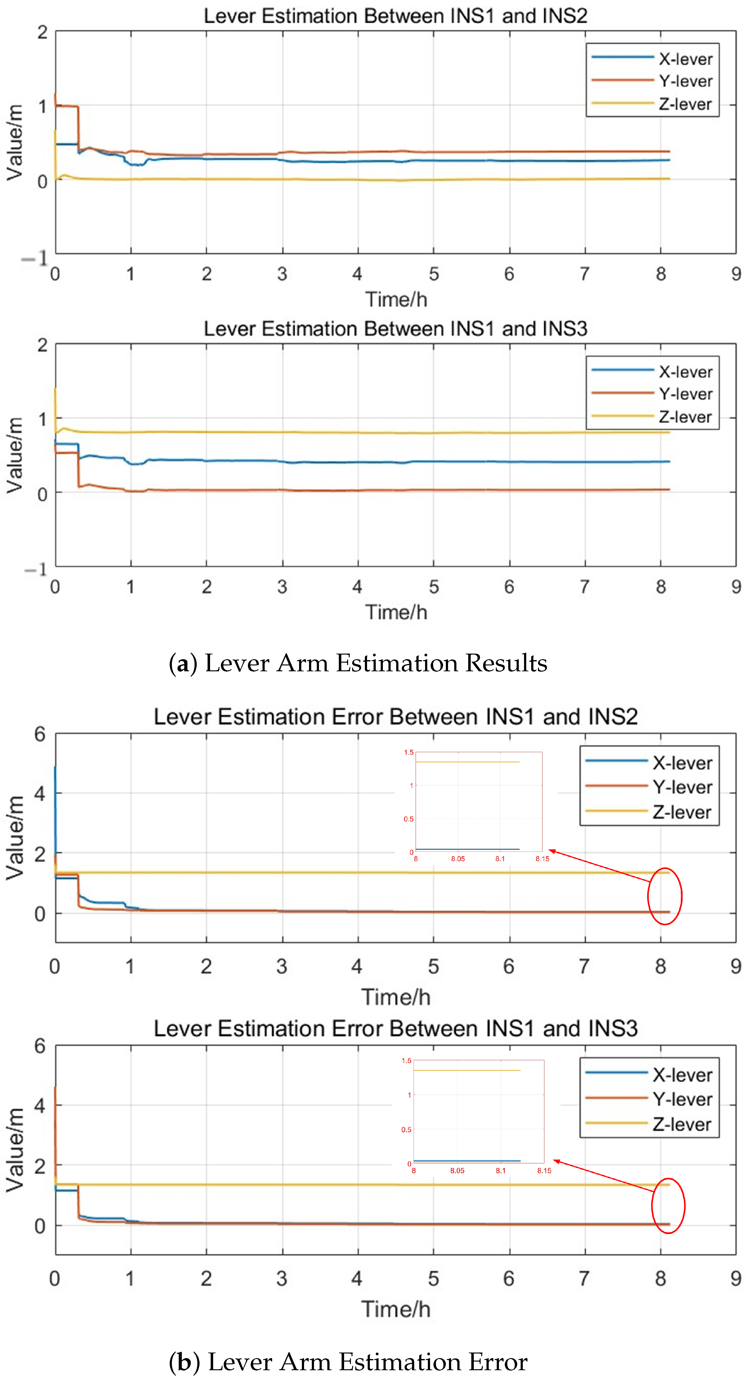
| Item | Simulation Experiment | Estimation Error | |
|---|---|---|---|
| SRINS1 and SRINS2 | x-axis | 0.2596 m | 0.0046 m |
| y-axis | 0.3749 m | −0.0001 m | |
| z-axis | 0.0117 m | 0.0117 m | |
| SRINS1 and SRINS3 | x-axis | 0.3990 m | −0.0100 m |
| y-axis | 0.0192 m | 0.0108 m | |
| z-axis | 0.7925 m | 0.0075 m | |
| Item | Positioning Error (RMS) | |||
|---|---|---|---|---|
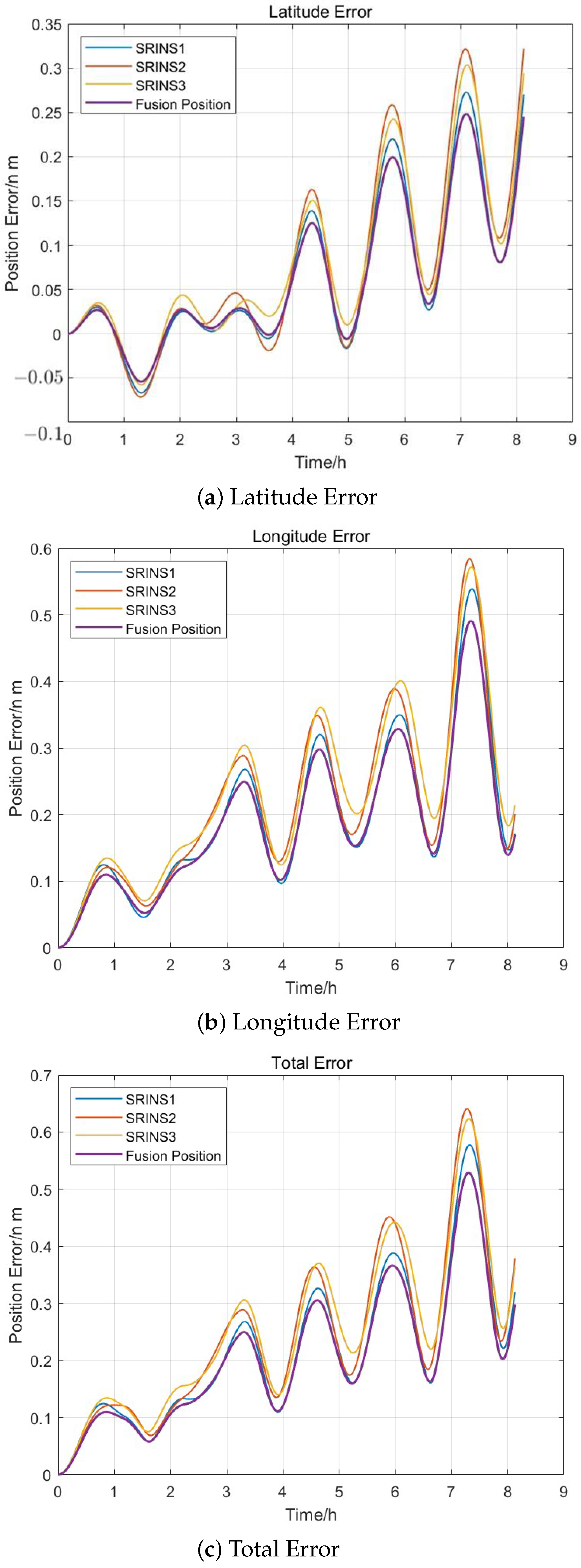
| Longitude Error | Latitude Error | Total Error | ||
| Simulation Experiment | SRINS1 | 0.1058 n m | 0.2283 n m | 0.2516 n m |
| SRINS2 | 0.1272 n m | 0.2514 n m | 0.2817 n m | |
| SRINS3 | 0.1196 n m | 0.2609 n m | 0.2870 n m | |
| Data Fusion Result | 0.09740 n m | 0.2145 n m | 0.2356 n m | |
| Accuracy Increase | 7.9785% | 6.0212% | 6.3645% | |
| Item | SRINS1 | SRINS2 | SRINS3 | |
|---|---|---|---|---|
| Laser gyroscope bias stability (100-s smoothing) | x-axis gyroscope | /h | /h | /h |
| y-axis gyroscope | /h | /h | /h | |
| z-axis gyroscope | /h | /h | /h | |
| Quartz flexible accelerometer bias stability (100-s smoothing) | x-axis accelerometer | g | g | g |
| y-axis accelerometer | g | g | g | |
| z-axis accelerometer | g | g | g | |
| Item | The First Experiment | The Second Experiment | |
|---|---|---|---|
| SRINS1 and SRINS2 | x-axis | 0.7305 m | 0.6800 m |
| y-axis | 0.8838 m | 0.9146 m | |
| z-axis | 0.0314 m | 0.0302 m | |
| SRINS1 and SRINS3 | x-axis | −0.3975 m | −0.4069 m |
| y-axis | 0.5823 m | 0.6060 m | |
| z-axis | 0.0127 m | 0.0164 m | |
| Item | Positioning Error (RMS) | |||
|---|---|---|---|---|
| Longitude Error | Latitude Error | Total Error | ||
| The First Trial | SRINS1 | 0.2989 n m | 0.2799 n m | 0.4095 n m |
| SRINS2 | 0.3212 n m | 0.2228 n m | 0.3909 n m | |
| SRINS3 | 0.3747 n m | 0.2497 n m | 0.4503 n m | |
| Data Fusion Result | 0.2801 n m | 0.2084 n m | 0.3491 n m | |
| Accuracy Increase | 6.3180% | 6.4684% | 10.6943% | |
| The Second Trial | SRINS1 | 0.4854 n m | 0.4904 n m | 0.6900 n m |
| SRINS2 | 0.4852 n m | 0.5935 n m | 0.7666 n m | |
| SRINS3 | 0.4630 n m | 0.3933 n m | 0.6075 n m | |
| Data Fusion Result | 0.4141 n m | 0.3643 n m | 0.5516 n m | |
| Accuracy Increase | 10.5539% | 7.3664% | 9.2041% | |
| Average Accuracy Increase | 8.4360% | 6.9174% | 9.9492% | |
Disclaimer/Publisher’s Note: The statements, opinions and data contained in all publications are solely those of the individual author(s) and contributor(s) and not of MDPI and/or the editor(s). MDPI and/or the editor(s) disclaim responsibility for any injury to people or property resulting from any ideas, methods, instructions or products referred to in the content. |
© 2024 by the authors. Licensee MDPI, Basel, Switzerland. This article is an open access article distributed under the terms and conditions of the Creative Commons Attribution (CC BY) license (https://creativecommons.org/licenses/by/4.0/).
Share and Cite
Xiong, Y.; Yang, G.; Wen, Z. A Method to Improve Underwater Positioning Reference Based on Topological Distribution Constraints of Multi-INSs. Appl. Sci. 2024, 14, 10206. https://doi.org/10.3390/app142210206
Xiong Y, Yang G, Wen Z. A Method to Improve Underwater Positioning Reference Based on Topological Distribution Constraints of Multi-INSs. Applied Sciences. 2024; 14(22):10206. https://doi.org/10.3390/app142210206
Chicago/Turabian StyleXiong, Yuyu, Gongliu Yang, and Zeyang Wen. 2024. "A Method to Improve Underwater Positioning Reference Based on Topological Distribution Constraints of Multi-INSs" Applied Sciences 14, no. 22: 10206. https://doi.org/10.3390/app142210206
APA StyleXiong, Y., Yang, G., & Wen, Z. (2024). A Method to Improve Underwater Positioning Reference Based on Topological Distribution Constraints of Multi-INSs. Applied Sciences, 14(22), 10206. https://doi.org/10.3390/app142210206