A Dynamic Edge Server Placement Scheme Using the Improved Snake Optimization Algorithm

Abstract

In the paradigm of mobile edge computing (MEC), providing low-latency and high-reliability services for users is garnering increasing attention. Appropriate edge-server placement is the crucial first step to realizing such services, as it can meet computation requirements and enhance resource utilization. This study delves into efficient and intelligent dynamic edge-server placement by taking into account time-varying network scenarios and deployment costs. Firstly, edge servers are classified into static and dynamic ones. Subsequently, an improved snake optimization algorithm is proposed to determine the number and placement locations of dynamic servers while adhering to delay requirements. Finally, a minimum placement-cost algorithm is put forward to further reduce the service cost. Experimental results demonstrate that compared to classic algorithms, the proposed algorithms can achieve a reduction in latency of 5% to 12%. And compared to the state-of-the-art methods, they can reduce service costs by 20% to 43%. This research offers an effective solution for dynamic edge-server placement and holds great theoretical and practical significance.

1. Introduction

In the 5G/6G era, mobile edge computing (MEC) has emerged as a computing architecture enabler, as this technique migrates computing from the core network to the network edge [1]. As a result, MEC significantly reduces transmission latency and improves the user’s quality of experience [2].

Edge servers are the key elements of MEC [3]; they provide resources for processing data and tasks and are deployed closer to users than the core network server. However, it is difficult to determine the required number of edge servers and their deployment locations based on the deployment cost and desired performance, including the required delay, energy efficiency, and system reliability [4]. Providing full coverage for all users is not always feasible. Further, deploying edge servers in areas far from users induces resource waste and high costs, but deployment of only a small number of edge servers in dense areas degrades the user service experience. Most previous studies on this problem focused on static edge-server placement only, in which the locations are fixed once the edge servers are deployed [4,5]. However, edge-server placement should be dynamically adjusted to handle changing conditions such as variations in demand, cost, and efficiency.

To overcome these challenges, this study explores efficient and intelligent dynamic edge-server placement by considering time-varying network scenarios and deployment costs.

The main contributions of this paper can be summarized as follows:

•

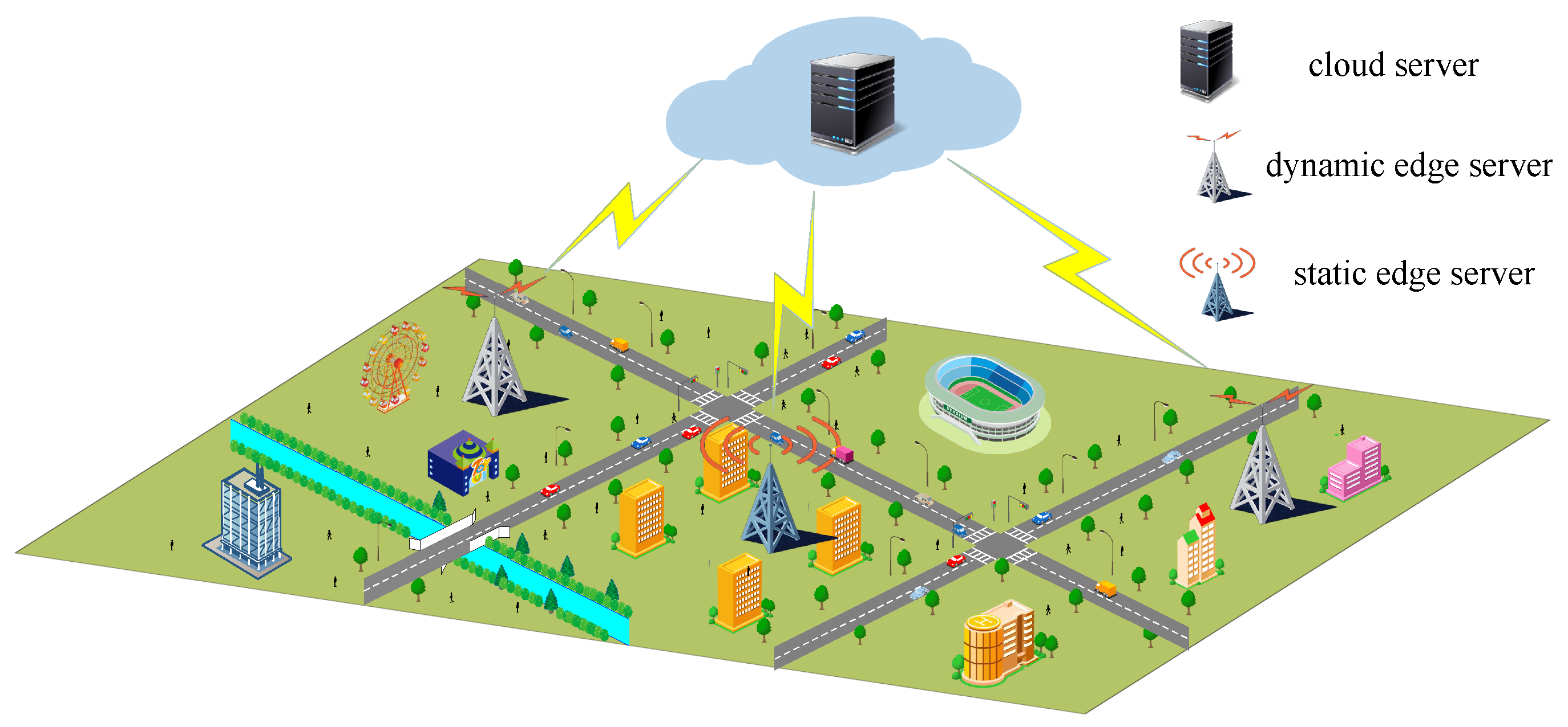
The edge servers are classified as static or dynamic. Static servers are deployed in densely populated areas, whereas dynamic servers move over time in response to dynamic changes in user locations; the number of dynamic servers can be increased or decreased.

•

The snake optimization (SO) algorithm [6] is improved to determine the optimal server placement and to implement operations such as increasing, decreasing, and moving the servers via a dynamic edge-server placement algorithm. The minimum placement-cost algorithm is used to calculate the minimum edge-server movement distance.

The rest of this paper is organized as follows. Firstly, we review the related work in Section 2. Then, we present the system model and problem description in Section 3. In Section 4, we propose the algorithm for dynamic placement of edge servers. Additionally, we provide simulation results and analysis in Section 5. Finally, conclusions and future perspectives are presented in Section 6.

2. Related Work

Edge-server location selection is a combinatorial optimization problem, the computational complexity of which grows exponentially with the problem size [7]. To tackle this challenge, previous studies have employed various optimization algorithms, including spatial clustering [8,9], integer linear programming [10,11], game theory [12], bionic intelligence [13,14], and heuristic [3] algorithms.

In terms of static placement, a deep reinforcement learning-based multi-objective edge server placement strategy was previously proposed for the performance of a vehicular networking task [15]; this approach was designed to improve the coverage and workload balance and reduce the average latency. Additionally, Ling et al. [16] formulated the edge-server placement problem as a constrained optimization problem and decreased the network latency and energy consumption via a particle swarm optimization (PSO) algorithm. As a result, the total edge-server cost was reduced. In another work, the server deployment and resource allocation were optimized to achieve low latency and load balancing. This was achieved through subregion partitioning, the whale optimization algorithm, neural networks, and game theory [17]. Finally, Wang et al. [18] employed a fault tolerance mechanism and a binary-based gray-wolf genetic policy algorithm for edge-server deployment; this approach ensured normal system operation in case of failures.

In terms of dynamic placement, a non-dominated sequential genetic algorithm was previously employed to reconstruct existing locations [19]. In that work, the minimum reconstruction cost was computed based on the Kuhn–Munkres two-part graph matching algorithm. Further, Jiang et al. [20] employed proximity policy optimization to reduce the total server placement cost, and used heat and grey-scale maps to convert the network states into network inputs.

In the mentioned dynamic placement methods, some have poor scalability, requiring consideration of all edge servers each time deployment is adjusted [19]. Some have high deployment costs [20]. In this paper, by categorizing edge servers into static servers and dynamic servers, only the operations such as addition and movement of dynamic servers need to be considered during each adjustment. This approach reduces deployment costs and improves scalability.

3. System Modeling and Problem Description

System models for dynamic edge-server placement include network, coverage, delay, and cost models. In detail, a network model considers the network connectivity between the mobile users and edge servers, a coverage model considers the edge-server service range and coverage capability, a latency model focuses on the communication latency between the edge servers and users, and a cost model considers the fixed and mobile edge-server costs. These four models are introduced below.

3.1. Network Model

This study considers a scenario where end devices directly send task data to cloud or edge servers, as shown in Figure 1. We consider M static edge servers $E_i^s$, which are placed in densely populated areas, where $i=\{1,2,\dots ,M\}$. Additionally, N dynamic edge servers $E_j^d$ are used to improve the system performance, where $j=\{1,2,\dots ,N\}$. Furthermore, there are Z users $D_k$ randomly placed in the scenario, where $k=\{1,2,\dots ,Z\}$.

3.2. Coverage Model

The edge-server coverage model aims to achieve efficient task processing and distribution to improve the system performance and user experience. This model considers the random generation of differently sized task datasets performed by each user, as well as the different computing abilities and coverage capacities of the edge and cloud servers. In this model, to promote synergy between the cloud and edge, the cost is minimized while ensuring quality of service. An effective strategy is to deploy edge servers in crowded places but to allow users in sparsely populated places to directly offload tasks to the cloud servers for processing.

Assuming that the edge-server coverage radius is r, a user is covered by the edge server when the distance d between the user and edge server is less than r. The Haversine formula can be used to calculate d. Taking the user latitude and longitude coordinates as $(la{t}_1,lo{n}_1)$ and the edge-server latitude and longitude coordinates as $(la{t}_2,lo{n}_2)$, we obtain

$$d=2r\times arcsin\left(\sqrt{{sin}^2\left(A\right)+C{sin}^2\left(B\right)}\right),$$

(1)

where $A=(la{t}_2-la{t}_1)/2$, $B=(lo{n}_2-lo{n}_1)/2$, $C=cos\left(la{t}_1\right)cos\left(la{t}_2\right)$.

When a user is covered by an edge server, the user’s tasks are offloaded to the nearest edge server for processing in order to reduce data transmission latency. When a user is not covered by an edge server, their tasks are offloaded to a cloud server for processing. It is important to note that if an edge server reaches its computing capacity limit $\mu$ due to the arrival data volume $\eta$, even if it covers the user, the tasks cannot be offloaded to that particular edge server. In such cases, the user has the option to offload the tasks to the nearest edge server or cloud server that has not reached its computing capacity limit and can cover the user.

3.3. Delay Model

The latency mainly refers to the transmission delay when the user offloads data to the edge or cloud servers.

We assume that ${\delta }_k$ is the volume of data to be offloaded from each IoT end device $D_k$ and take ${\alpha }_k$ as the offloading decision variable, where ${\alpha }_k\in \{0,1\}$. When ${\alpha }_k=0$, $D_k$ does not select the edge server for task offloading; when ${\alpha }_k=1$, $D_k$ offloads all the task data to the edge server for processing. Therefore, the total volume of task data ${\lambda }_k$ that the user offloads to the edge server for processing is

$${\lambda }_k={\alpha }_k{\delta }_k.$$

(2)

When the user offloads task data to the edge server, the transmission rate $r_k^e$ of the kth user offloading the task to the edge server is calculated using Shannon’s formula. The calculation formula is

$$r_k^e=\mathrm{w}\times {log}_2\left(1+{\displaystyle \frac{P\times l_k^{-\alpha }\times h_1}{N_0}}\right),$$

(3)

where w denotes the channel bandwidth, P denotes the Internet of Things (IoT) terminal transmission power, $l_k$ denotes the distance between the kth IoT terminal and edge server, $\alpha$ denotes the path loss factor, $h_1$ denotes the channel gain between the user and edge server, and $N_0$ denotes the noise power.

Therefore, the transmission latency $T_e$ when users offload task data to the edge server can be expressed as follows

$$T_e=\sum _{k=1}^Z{\displaystyle \frac{{\lambda }_k}{r_k^e}}.$$

(4)

When users offload task data to the cloud server for processing, the transmission rate $r_k^c$ can be calculated using Shannon’s formula. The calculation formula is as follows

$$r_k^c=\mathrm{w}\times {log}_2\left(1+{\displaystyle \frac{P\times l^{-\alpha }\times h_2}{N_0}}\right),$$

(5)

here, l and $h_2$ denote the distance and channel gain between the user and cloud server, respectively. Therefore, the transmission delay for all users to offload their task data to the cloud server $T_c$ is expressed as

$$T_c=\sum _{k=1}^Z{\displaystyle \frac{{\lambda }_k}{r_k^c}}.$$

(6)

Thus, the average latency of offloading task data to the edge or cloud server for all users T is expressed as

$$T={\displaystyle \frac{T_e+T_c}{z}}.$$

(7)

3.4. Cost Model

As noted above, edge servers can be categorized as static or dynamic. Static edge servers do not move once placed, whereas dynamic edge servers can be moved. The edge-server placement cost has three main components: the fixed, compensation, and dynamic costs. The fixed cost is that for edge-server purchasing and deployment. The compensation cost refers to the fact that idle edge servers can be used for other purposes to compensate for the deployment cost. The dynamic cost is that incurred by the edge servers as a result of location changes.

User latency exceeding the given threshold indicates a small number of edge servers; the number of mobile edge servers must be increased to reduce this latency. The incurred cost of the newly deployed edge servers is

$$C_1=\left\{\begin{array}{cc}(n_{t+1}-n_t)(\omega +\theta ),\hfill & \mathrm{if}{n}_{t+1}>n_t\hfill \\ 0,\hfill & \mathrm{otherwise}\hfill \end{array}\right.,$$

(8)

where $\omega$ denotes the cost of purchasing an edge server, $\theta$ denotes the cost of deploying each edge server, and $n_{t+1}$ denotes the number of dynamic edge servers at time $t+1$.

When the user latency is below a certain value, this indicates that too many edge servers are deployed. Then, some of the edge servers can be used for other purposes to compensate for the deployment cost. The compensation cost is computed as follows

$$C_2=\left\{\begin{array}{cc}(n_t-n_{t+1})\psi ,\hfill & \mathrm{if}{n}_t>n_{t+1}\hfill \\ 0,\hfill & \mathrm{otherwise}\hfill \end{array}\right.,$$

(9)

where $\psi$ denotes the benefit available to each idle edge server.

When an edge server must be moved, the dynamic cost includes the dismantling cost at the previous location, the installation cost at the new location, and the edge-server movement cost. The dynamic cost is calculated as

$$C_3=2\theta n_m+\zeta W,$$

(10)

where $n_m$ denotes the number of edge servers that must be moved, $\zeta$ denotes the cost per unit distance that the edge server must be moved, and W denotes the minimum distance that all edge servers must be moved. Here

$$\begin{array}{c}{n}_m=min(N_{t+1}-(N_{t+1}\cap N_t), N_t-(N_{t+1}\cap N_t)),\hfill \end{array}$$

(11)

where $N_{t+1}$ represents the set of edge server locations at time $t+1$, and $N_t$ represents the set of edge server locations at time t.

In summary, the total cost of edge-server placement is

$$C=C_1-C_2+C_3.$$

(12)

3.5. Problem Description

This study aims to determine the optimal edge-server number and placement according to conditional variations, where the edge-server number and placement are constrained by a certain desired latency range and are determined by factors such as the network model, edge coverage, and user latency. The problem can be modeled as follows

$$minC$$

(13)

s.t.

$$\lambda <\sum _{k=1}^Z{\delta }_k$$

(14)

$$\eta \le \mu$$

(15)

$$T_{min}\le T\le T_{max}$$

(16)

Constraint (14) indicates that the task data processed at the edge server is less than the sum of the data for all users, Constraint (15) indicates that the user data received by the edge server requires processing that is within the computational capacity of the edge server, and Constraint (16) indicates that the computed average user latency satisfies the defined range.

4. Dynamic Edge-Server Placement

Dynamic edge-server placement involves several steps. In the approach proposed herein, the optimal edge-server placement for the current moment is calculated using the improved SO (ISO) algorithm. Next, the dynamic edge-server placement algorithm is used to adjust the number of edge servers and their locations in accordance with the environment changes. Then, the minimum movement cost between the edge-server placement at the current moment and that at the next moment is derived based on the minimum placement-cost algorithm. Finally, the total cost at the next moment is computed. To optimize the placement of edge servers for the ISO algorithm, we employed a mapping strategy that transforms multiple unrelated variables into coordinates representing the positions. Specifically, we used the first and second dimensions of the algorithm variable ‘dim’ to determine the coordinates of the first position, and the third and fourth dimensions to determine the coordinates of the second position, and so on. By employing this mapping approach, we were able to convert the original multidimensional optimization problem into a two-dimensional problem within the spatial domain. This allowed us to utilize the ISO algorithm to search for optimal solutions in this two-dimensional space.

4.1. Snake Optimization Algorithm

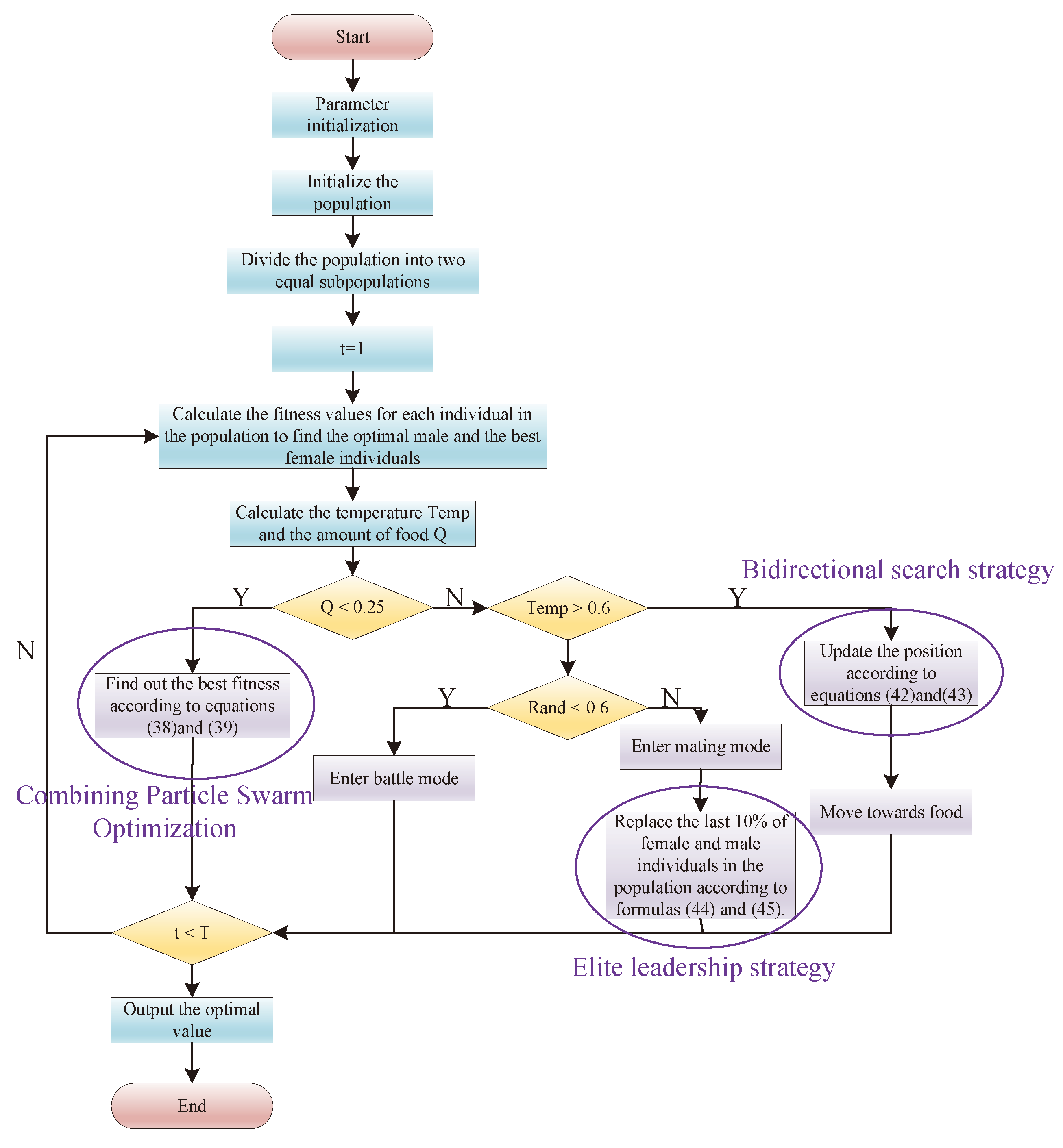
The SO algorithm is a novel meta-heuristic optimization algorithm that simulates the behavioral patterns of snakes under different temperatures and food conditions for optimal value finding. The SO algorithm is initialized with a given population; that is, N individuals are randomly generated as the original population in the search space, as follows

$$X_i=X_{min}+r\times (X_{max}-X_{min}),$$

(17)

where r is a random number between 0 and 1, $X_i$ is the ith individual in the population, and $X_{max}$ and $X_{min}$ are the upper and lower bounds of the value range for the optimization problem, respectively. Subsequently, the population is divided into two sub-populations, females and males, using the following two equations

$$N_m\approx {\displaystyle \frac{N}{2}}$$

(18)

$$N_f\approx N-N_m,$$

(19)

where $N_m$ and $N_f$ are the numbers of male and female individuals, respectively. The temperature is defined as

$$Temp=exp({\displaystyle \frac{-t}{X}}),$$

(20)

where t is the current iteration number, and X is the maximum iteration number. The number of food items is defined as

$$Q=c_1\times exp({\displaystyle \frac{t-X}{X}}),$$

(21)

where $c_1$ is a constant. When $Q<\mathrm{Threshold}1$, the snake searches for food by choosing any random position and updates its position according to the following equations

$$\begin{array}{c}{X}_{i,m}(t+1)=X_{rand,\mathrm{m}}\left(t\right)\pm c_2\times A_m\times ((X_{max}-X_{min})\times rand+X_{min})\hfill \end{array}$$

(22)

$$\begin{array}{c}{X}_{i,f}(t+1)=X_{rand,f}\left(t\right)\pm c_2\times A_f\times ((X_{max}-X_{min})\times rand+X_{min}),\hfill \end{array}$$

(23)

where $X_{i,m}$ and $X_{i,f}$ represent the positions of the ith male and female snakes, respectively, and $X_{rand,\mathrm{m}}$ and $X_{rand,f}$ represent the randomly selected positions of male and female snakes. $A_m$ and $A_f$ represent the ability of male and female snakes to find food, and $c_2$ takes the value of 0.05. The calculation methods of $A_m$ and $A_f$ are as follows

$$A_m=exp({\displaystyle \frac{-f_{rand,m}}{f_{i,m}}})$$

(24)

$$A_f=exp({\displaystyle \frac{-f_{rand,f}}{f_{i,f}}}),$$

(25)

where $f_{\mathrm{rand},m}$ and $f_{\mathrm{rand},f}$ are the fitness values of $X_{\mathrm{rand},m}$ and $X_{\mathrm{rand},f}$, respectively, and $f_{i,m}$ and $f_{i,f}$ are the fitness values of $X_{i,m}$ and $X_{i,f}$, respectively. When $Q>\mathrm{Threshold}1$, if $\mathrm{Temperature}>\mathrm{Threshold}2$, the snake goes to search for food and the position update equations are as follows

$$X_{i,m}(t+1)=X_{food}\pm c_3\times Temp\times rand\times (X_{food}-X_{i,m}\left(t\right))$$

(26)

$$X_{i,f}(t+1)=X_{food}\pm c_3\times Temp\times rand\times (X_{food}-X_{i,f}\left(t\right)),$$

(27)

where $X_{i,m}$ and $X_{i,f}$ are the positions of the ith male and female snakes, respectively, $X_{\mathrm{food}}$ is the position of the best-performing individual, and $c_3$ takes a value of 2. If $\mathrm{Temperature}<\mathrm{Threshold}2$, the snake is randomly in fight or mate mode. When the snake is in fight mode, the position update equation is:

$$X_{i,m}(t+1)=X_{i,m}\left(t\right)+c_3\times FM\times rand\times (Q\times X_{best,f}-X_{i,m}\left(t\right))$$

(28)

$$X_{i,f}(t+1)=X_{i,f}\left(t\right)+c_3\times FF\times \mathrm{rand}\times (Q\times X_{\mathrm{best},m}-X_{i,f}\left(t\right)),$$

(29)

where $X_{\mathrm{best},m}$ and $X_{\mathrm{best},f}$ are the positions of the optimal individuals among the males and females, respectively, and $FM$ and $FF$ are the fighting abilities of the males and females, respectively. Here,

$$FM=exp({\displaystyle \frac{-f_{best,f}}{f_i}})$$

(30)

$$FF=exp({\displaystyle \frac{-f_{best,m}}{f_i}}),$$

(31)

where $f_{\mathrm{best},m}$ and $f_{\mathrm{best},f}$ are the fitness values of the best-performing individuals among the male and female snakes, respectively, and $f_i$ is the fitness of individual i. When the snake is in mating mode, the position update equations are:

$$X_{i,m}(t+1)=X_{i,m}\left(t\right)+c_3\times M_m\times rand\times (Q\times X_{i,f}\left(t\right)-X_{i,m}\left(t\right))$$

(32)

$$X_{i,f}(t+1)=X_{i,f}\left(t\right)+c_3\times M_f\times rand\times (Q\times X_{i,m}\left(t\right)-X_{i,f}\left(t\right)),$$

(33)

where $M_m$ and $M_f$ denote the mating abilities of the male and female snakes, respectively. Here,

$$M_m=exp({\displaystyle \frac{-f_{i,f}}{f_{i,m}}})$$

(34)

$$M_f=exp({\displaystyle \frac{-f_{i,m}}{f_{i,f}}}),$$

(35)

where $f_{i,m}$ and $f_{i,f}$ are the fitness values of the ith male and female snakes, respectively. After mating is complete, egg hatching may be selected. If hatching is chosen, the worst-performing male and female individuals in the population are selected for replacement:

$$X_{worst,m}=X_{min}+rand\times (X_{max}-X_{min})$$

(36)

$$X_{worst,f}=X_{min}+rand\times (X_{max}-X_{min}),$$

(37)

here, $X_{worst,m}$ and $X_{worst,f}$ are the worst-performing individuals among the male and female snakes, respectively.

4.2. ISO Algorithm

To improve the performance of the SO algorithm, this study adds the concept of the PSO algorithm to improve the global search ability. In addition, we invoke the two-way search strategy to enhance the algorithm optimization ability and incorporate the concept of elite leading to aid the excellent individuals in spreading their information. The experiment results show that, compared with the original SO algorithm, the ISO algorithm converges faster and has better adaptability. Figure 2 is the ISO algorithm flowchart.

4.2.1. Combination with PSO

The SO algorithm uses the random search approach to explore the region in the early iterations; however, the uncertainty is high. The PSO algorithm has a higher convergence speed in the early iterations. Therefore, the SO algorithm can be improved by combining it with the PSO algorithm in the pre-iteration period. The improvement measures are as follows.

In the PSO algorithm, the position update equation for male individuals and female individuals is to add the velocity of the next step to the current position.

$$X_{i,m}(t+1)=X_{i,m}\left(t\right)+V_{i,m}(t+1)$$

(38)

$$X_{i,f}(t+1)=X_{i,f}\left(t\right)+V_{i,f}(t+1),$$

(39)

where $X_{i,m}$ and $X_{i,f}$ represent the positions of male and female individuals, respectively, in generation t. $V_{i,m}(t+1)$ and $V_{i,f}(t+1)$ represent the velocities of male and female individuals, respectively, in generation $t+1$. The update formula for these velocities is as follows:

$$\begin{array}{c}{V}_{i,m}(t+1)=\omega \times V_{i,m}\left(t\right)+c_1\times rand\times (P_{i,pbestm}\left(t\right)\hfill \\ -X_{i,m}\left(t\right))+c_2\times rand\times (P_{gbestm}\left(t\right)-X_{i,m}\left(t\right))\hfill \end{array}$$

(40)

$$\begin{array}{c}{V}_{i,f}(t+1)=\omega \times V_{i,f}\left(t\right)+c_1\times rand\times (P_{i,pbestf}\left(t\right)\hfill \\ -X_{i,f}\left(t\right))+c_2\times rand\times (P_{gbestf}\left(t\right)-X_{i,f}\left(t\right)),\hfill \end{array}$$

(41)

where $\omega$ is the inertia weight, $V_{i,m}\left(t\right)$ and $V_{i,f}\left(t\right)$ represent the velocities of male and female individuals, respectively, in generation t. $P_{i,pbestm}\left(t\right)$ and $P_{i,pbestf}\left(t\right)$ represent the personal best solutions of the ith male and female individuals, respectively, after t iterations. $P_{gbestm}\left(t\right)$ and $P_{gbestf}\left(t\right)$ represent the global best solutions in the entire male and female population, respectively, after t iterations.

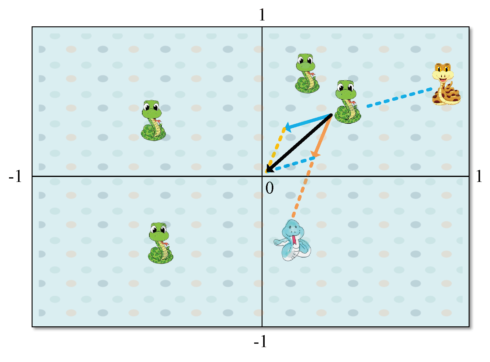
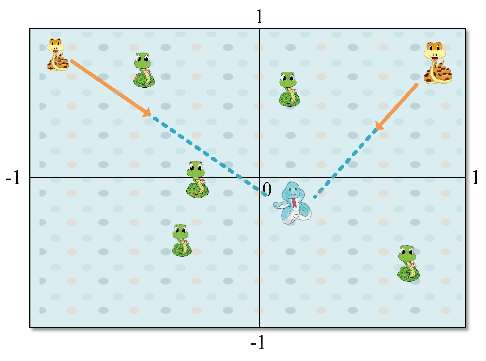
4.2.2. Bidirectional Search Strategy

When Temperature >Threshold2, the snake enters a small-scale search mode to find food. The original algorithm has a weak ability to find the optimal solution in this process. At this point, however, the ability to find the local optimal solution can be increased by using the bidirectional search strategy: a strategy that utilizes the best- and worst-performing individuals to explore within the search area. This approach is designed to keep the algorithm from the worst-performing individual while remaining close to the best-performing individual. The position update equations are

$$\begin{array}{c}{X}_{i,m}(t+1)=X_{i,m}\left(t\right)+r_1\times (X_{m,best}-X_{i,m}\left(t\right))-r_2\times (X_{m,worst}-X_{i,m}\left(t\right))\hfill \end{array}$$

(42)

$$\begin{array}{c}{X}_{i,f}(t+1)=X_{i,f}\left(t\right)+r_1\times (X_{f,best}-X_{i,f}\left(t\right))-r_2\times (X_{f,worst}-X_{i,f}\left(t\right)),\hfill \end{array}$$

(43)

where $X_{m,best}$ and $X_{m,worst}$ denote the best- and worst-performing males, respectively, and $X_{f,best}$ and $X_{f,worst}$ denote the best- and worst-performing females, respectively. The bidirectional search approach allows the algorithm to approach the optimum while fully utilizing the search space; hence, the algorithm convergence is accelerated.

The strategy is visualized in Figure 3 and Figure 4, taking the two-dimensional space as an example. This figure is a distribution map of the positions of six individuals at a given moment. A position closer to the zero point of the coordinate axis represents a better fitness value. The blue and brown snakes represent the best- and worst-performing individuals, respectively; the remaining individuals are represented by green snakes. When using the bidirectional search strategy, the position of one of the snakes changes, as shown in Figure 3 and Figure 4, where the orange and blue lines in Figure 3 indicate that the individual is moving closer to and away from the best- and worst-performing individuals, respectively. The black line indicates the final movement direction and distance of this individual under the influence of the best- and worst-performing individuals. Figure 4 shows the position distribution of the individual after movement. The moving individual becomes the best-adapted individual, and the original best-adapted individual is classed among the remaining individuals.

4.2.3. Elite Leadership Strategy

The SO algorithm incorporates a certain probability that the snakes will produce eggs after mating, i.e., that the worst solution will be replaced by a randomly generated solution. However, the blindness of the randomized solution reduces the ability of the algorithm to find the optimal solution quickly. Therefore, the elite leadership strategy is adopted in this study. This strategy replaces the 10% of the individuals with the lowest fitness in the algorithm to increase the probability of finding the optimal solution. The equations are

$$X_{i,m}(t+1)=X_{i,m}\left(t\right)+r_1\times (X_{m,gbest}-X_{i,m}\left(t\right))$$

(44)

$$X_{i,f}(t+1)=X_{i,f}\left(t\right)+r_1\times (X_{f,gbest}-X_{i,f}\left(t\right)),$$

(45)

where $X_{m,gbest}$ and $X_{f,gbest}$ denote the optimal individuals among all males and females, respectively. This improvement can avoid the blindness of the random solution, improve the algorithm convergence speed and quality, and increase the probability of finding the optimal solution.

Figure 5 and Figure 6 visualize this strategy. The position distributions of 11 individuals at a given moment are shown. The blue snake represents the best-adapted individual, the brown snakes represent the individuals with fitness values in the bottom 10%, and the remaining individuals are represented by green snakes. When the elite leading strategy is used, the brown-snake position changes as shown in Figure 5 and Figure 6. The blue line in Figure 5 indicates that the individual is moving closer to the best-performing individual; the orange line indicates the movement direction and distance of the individual. Figure 6 shows the position distribution of the individuals following the movement of those with fitness values in the bottom 10%. The original best-performing individual is now classed among the remaining individuals, and some of the original remaining individuals are now among the individuals with fitness values in the bottom 10%.

The time complexity of the SO algorithm is O(TNd). The time complexity of combining with the PSO algorithm is O(N). The bidirectional search strategy does not increase the time complexity. The time complexity of the elite leading strategy is O(Nd). In conclusion, the final time complexity of the ISO algorithm is O((T + 1)Nd + N). Algorithm 1 describes the optimization process of the ISO algorithm.

Algorithm 1 Improved Snake Optimization Algorithm

Inputs: Maximum number of iterations, population size, etc.

Output: Optimal value

1: Initialize the edge server location

2: while $(t<T)$ do

3:    Calculate temp, Q, Xworst_m, Xworst_f, pBestm, gBestm, pBestf, gBestf

4:    if $(Q<Threshold1)$ then

5:      Find food, update position according to Equations (38) and (39)

6:    else

7:      if $(Q>Threshold2)$ then

8:         Move towards food and update position according to Equations (42) and (43)

9:      else

10:         if $(rand>0.6)$ then

11:           Enter combat mode and update position according to Equations (28) and (29)

12:         else

13:           Enter mating mode and update position according to Equations (32) and (33)

14:           Select whether to hatch or not; if hatching, update the position according to Equations (44) and (45)

15:         end if

16:      end if

17:    end if

18: end while

4.3. Dynamic Edge-Server Placement Algorithm

This section describes the proposed dynamic and intelligent edge-server placement strategy. Initially, we place static edge servers in areas where the population is relatively fixed and dense. Dynamic edge servers are then deployed so that the average user latency is within a certain range. However, because of the variations in the user locations over time, the user delay also varies. When the average user delay exceeds a certain range, we take appropriate reduction measures. First, we try to reduce the average user latency by adjusting the location of the dynamic edge server. If this approach fails to meet our requirements, we increase the number of edge servers to ensure that the latency remains within an acceptable range. In contrast, when the average user latency is below a certain threshold, we force it within a certain range by reducing the number of dynamic edge servers. The reduced edge servers can be used for other purposes to compensate for the deployment cost. This flexibility enables dynamic deployment decisions based on real-time conditions.

The solution steps are listed in Algorithm 2. With this dynamic and intelligent edge-server deployment strategy, the servers can better adapt to changes in crowd location, and thus, the quality of the user experience is optimized.

Algorithm 2 Dynamic Edge-Server Placement Algorithm

Input: Location of user distribution at different moments

Output: Number and location of dynamic edge servers

1: Find the optimal location for static server placement using the ISO algorithm

2: for $\mathrm{Time}=1$ to t do

3:    Optimize the dynamic-server placement using the ISO algorithm

4:    if $\min <\mathrm{delay}<\max$ then

5:      do nothing

6:    else

7:      if $\mathrm{delay}>\max$ then

8:         Increase the number of dynamic servers

9:         Compute the position and delay using the ISO algorithm

10:     else

11:         Reduce the number of dynamic servers

12:         Calculate the position and delay using the ISO algorithm

13:      end if

14:    end if

15: end for

4.4. Minimum Movement Distance Based on Linear Programming Problem

When the positions of multiple dynamic servers are changed during the cost-process solution, the minimum movement distance from the original to the new position must be calculated for all moving edge servers. As shown in Figure 7, which presents the original and new locations of three moving edge servers, each edge server can choose one of the three new locations as its new location; thus, there is a variety of movement possibilities, as shown by the line segments in the figure. At this point, a movement scheme that minimizes the total distance moved by the edge servers must be found. This problem can be regarded as a linear programming problem and can be solved using the interior point method, the core concept of which is that the optimal solution is approached gradually by searching inside the feasible solution. Compared with the traditional step-by-step approach to boundary approximation, the interior point method avoids searching the entire feasible solution space by iterating over the points within the feasible solution; this approach effectively reduces the number of iterations and improves the solving efficiency. As a result, the interior point method is widely used to solve linear programming problems.

The interior point method can be used to calculate the minimum movement distance between two sets of points. In each iteration, the interior point method gradually approaches the optimal solution by calculating the gradient and Hessian matrix, solving for the Newton step and decrement and implementing line searching and solution vector updating. Finally, the minimum cost of placing edge servers at the current moment is obtained by calculating the minimum movement distance and combining the dynamic edge-server addition and deletion operations. The solution steps are listed in Algorithm 3.

Algorithm 3 Minimum Placement-Cost Algorithm Based on Interior Point Methods

Inputs: Original and new position matrices

Output: Minimum cost

1: while $i<\mathrm{max\_iter}$ do

2:    Calculate the gradient and Hessian matrix

3:    if $\lambda /2<\mathrm{tol}$ then

4:      break

5:    end if

6:    while $x+t·dx$ is not valid do

7:      $t\leftarrow t·\mu$

8:    end while

9:    $x\leftarrow x+t·dx$

10: end while

5. Experiment Results and Analysis

5.1. Dataset Processing

The proposed approach was verified in simulation experiments. The Shanghai Telecom base station dataset [21,22,23], which contains millions of data elements consisting of location and user Internet logs, etc., was used for these experiments. User Internet-access start and end points were provided by this dataset. Therefore, we preprocessed the dataset and selected the number of users accessing the Internet and their locations at 04:00, 08:00, 12:00, 16:00, 20:00, and 24:00 in a single day.

5.2. Parameterization

The parameters used for the experiments are listed in

Table 1. Experiment parameters.

Parameter	Retrieved Value
Channel bandwidth w	10 MHz
User transmission power P	$0.2$ W
Path loss factor $\alpha$	10
Channel gain between user and edge server $h_1$	0.1
Noise power $N_0$	1.6 × 10−11
Channel gain between user and cloud server $h_2$	0.98
Distance from user to cloud server l	1 × 106 m
The number of initial static servers N	10

. Among these parameters, $\alpha$, $h_1$, $h_2$, and $N_0$ generally take fixed values. When P is larger, the transmission rate is faster and the transmission delay is shorter. When l is larger, the transmission rate is slower and the transmission delay is shorter.

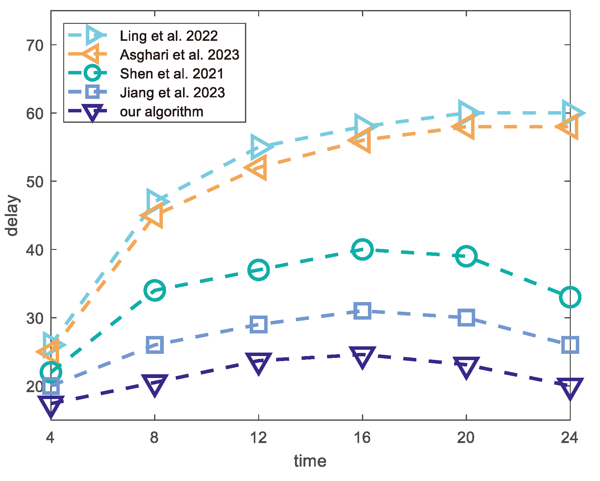
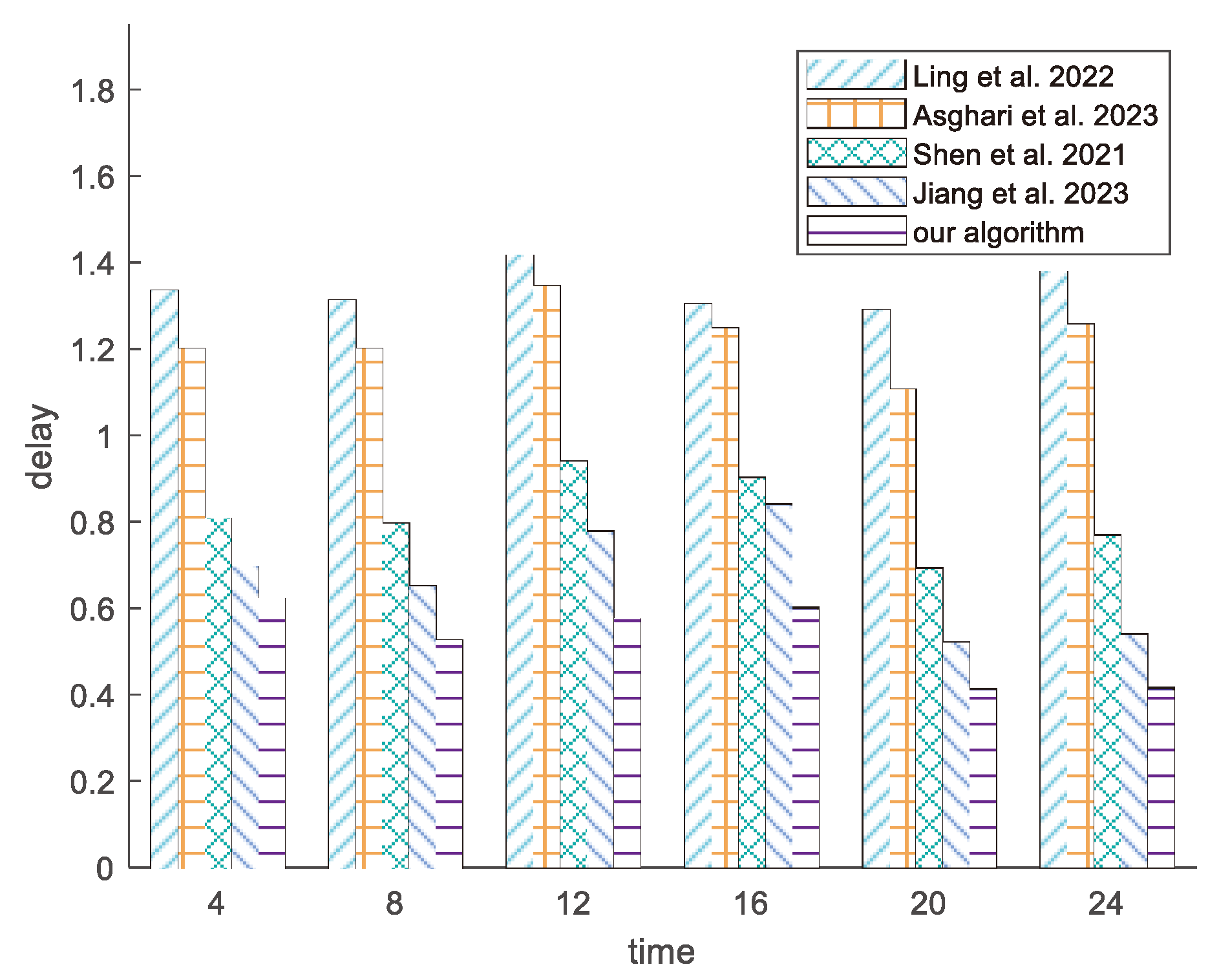
5.3. Experiment Results

The experimental process is as follows. First, map the user locations at the current time onto the map. Then, calculate the optimal placement locations and numbers of edge servers at the current time according to the ISO algorithm. As time passes and user locations change, recalculate the optimal placement locations and numbers of edge servers using the ISO algorithm and the dynamic edge-server placement algorithm. Next, calculate the minimum placement cost between this moment and the previous moment according to the minimum placement-cost algorithm, and set the edge servers that have not moved as static servers.

Figure 8 shows the cost values corresponding to different time points for various edge-server computing abilities. Clearly, the cost vs. time curves exhibit a decreasing trend as the edge-server computational ability increases. This is because the required number of edge servers decreases with increasing computational ability, which decreases the cost. Further, as the edge-server computational ability increases, the cost values grow closer. This is because, for low edge-server computing ability, some users within the edge-server coverage area are unable to offload their tasks to the server, and therefore, additional servers are required to fulfill the demand. However, as the computing ability increases, the number of additional servers required to compensate for a lack of computing ability decreases. Therefore, as the edge-server computational ability increases, the cost value gradually converges to a stable value.

Figure 9 shows the average user delay corresponding to different time points for various edge-server computational abilities. Clearly, the average user latency gradually decreases with increasing edge-server computational ability. This is because, when the edge-server computational ability is higher, more users can offload their tasks to the edge server for processing and not to the cloud; thus, the latency is reduced.

Figure 10 shows the cost values corresponding to different time points for various edge-server coverage values. Clearly, the costs corresponding to different time points exhibit a decreasing trend as the edge-server coverage increases. This is because an increase in coverage reduces the need for dynamic servers and, thus, the cost.

Figure 11 shows the average user delay corresponding to different time points for various edge-server coverage values. Clearly, the average user delay gradually decreases with increasing edge-server coverage. This is because increased edge-server coverage facilitates coverage of more users, who can offload their tasks to the edge servers for processing without relying on the cloud; thus, the latency is reduced.

Figure 12 shows the cost values corresponding to different time points for various values of the maximum number of tasks randomly generated by a user. Clearly, as the number of tasks increases, the cost vs. time curves exhibit an increasing trend. This is because, for increasing user tasks and a certain edge-server computational power, more edge servers are required to process the tasks, and thus, the cost is increased.

Figure 13 shows the average user delay values corresponding to different time points for various values of the maximum number of tasks randomly generated by the user. Clearly, as the number of tasks increases, the average user delay gradually increases. This is because, for a larger number of user-generated tasks, more time is required to offload the data to the cloud or edge servers, which increases the average user delay.

Based on the above experiments, the PSO, whale optimization algorithm (WOA), and SO algorithm were compared with our proposed algorithm in terms of latency. Additionally, the algorithms of Refs. [16,17,19,20] were compared with our proposed algorithm in terms of cost and average user latency. The results are reported below.

Figure 14 shows the average user latencies obtained for different algorithms and the same number of edge servers at 04:00. Clearly, the ISO algorithm has the smallest average user latency. Compared with other classic algorithms, the ISO algorithm can reduce the average user latency by approximately 5% to 12%. This indicates that the ISO algorithm determines the placement of edge servers more effectively, enabling more users to offload their tasks to the edge servers and thereby reducing the average user latency.

Figure 15 shows the cost values obtained for the different algorithms at different time points when the average delay was restricted to a certain range. Clearly, the algorithms in Refs. [16,17] had considerably higher costs than the dynamic placement algorithms; this is because they employ a static placement approach. Compared to the algorithms in Refs. [19,20], the algorithm proposed in this study minimized the cost by finding the minimum number of dynamic servers, optimal placement location, and minimum movement distance when the user location changed at different time points. Additionally, the latency was satisfactory, being within a reasonable range. Compared to the other algorithms, our approach yielded a cost reduction of 20% to 43%.

Figure 16 shows the average user delays corresponding to different time points for the different algorithms. The algorithms in Refs. [16,17] had considerably higher latency; again, this is because they are static algorithms, whereas the other algorithms are dynamic. Among the dynamic algorithms, the delay obtained for the algorithm developed in this study was consistently the lowest, which indicates that the proposed algorithm more efficiently determines the optimal edge-server placement.

6. Conclusions

In this study, we investigated the dynamic edge-server placement problem in a mobile edge computing environment. By improving the SO algorithm, we achieved an intelligent edge-server placement strategy to determine the optimal placement locations of edge servers. Experimental results show that our dynamic deployment method reduces latency by 5% to 12% compared to traditional algorithms while decreasing service costs by 20% to 43%. At the same time, the proposed minimum placement-cost algorithm effectively optimizes the deployment expenses of edge servers. Although the current research primarily focuses on optimizing latency and cost, practical applications may require balancing multiple objectives. Future work can incorporate multi-objective optimization, considering factors such as latency, cost, and energy consumption, to create a balance among these goals. It will further enhance the practicality and adaptability of dynamic edge-server placement schemes and provide stronger support for the development of the mobile edge computing field.

References

1. Cao, K.; Li, L.; Cui, Y.; Wei, T.; Hu, S. Exploring placement of heterogeneous edge servers for response time minimization in mobile edge-cloud computing. IEEE Trans. Ind. Inform. 2020, 17, 494–503. [Google Scholar] [CrossRef]
2. Singh, R.; Sukapuram, R.; Chakraborty, S. A survey of mobility-aware Multi-access Edge Computing: Challenges, use cases and future directions. Ad Hoc Netw. 2023, 140, 103044. [Google Scholar] [CrossRef]
3. Hou, P.; Li, B.; Wang, Z.; Ding, H. Joint hierarchical placement and configuration of edge servers in C-V2X. Ad Hoc Netw. 2022, 131, 102842. [Google Scholar] [CrossRef]
4. Chang, L.; Deng, X.; Pan, J.; Zhang, Y. Edge server placement for vehicular Ad Hoc networks in metropolitans. IEEE Internet Things J. 2021, 9, 1575–1590. [Google Scholar] [CrossRef]
5. Xu, X.; Shen, B.; Yin, X.; Khosravi, M.R.; Wu, H.; Qi, L.; Wan, S. Edge server quantification and placement for offloading social media services in industrial cognitive IoV. IEEE Trans. Ind. Inform. 2020, 17, 2910–2918. [Google Scholar] [CrossRef]
6. Hashim, F.A.; Hussien, A.G. Snake Optimizer: A novel meta-heuristic optimization algorithm. Knowl.-Based Syst. 2022, 242, 108320. [Google Scholar] [CrossRef]
7. Li, B.; Hou, P.; Wang, K.; Peng, Z.; Jin, S.; Niu, L. Deployment of edge servers in 5G cellular networks. Trans. Emerg. Telecommun. Technol. 2022, 33, e3937. [Google Scholar] [CrossRef]
8. Li, B.; Hou, P.; Wu, H.; Hou, F. Optimal edge server deployment and allocation strategy in 5G ultra-dense networking environments. Pervasive Mob. Comput. 2021, 72, 101312. [Google Scholar] [CrossRef]
9. Feng, C.; Yang, Q.; Quek, T.Q.S.; Wu, W.; Guo, K. Spatially-Temporally Collaborative Service Placement and Task Scheduling in MEC Networks. IEEE Trans. Veh. Technol. 2023, 72, 16650–16666. [Google Scholar] [CrossRef]
10. Chen, Y.; Lin, Y.; Zheng, Z.; Yu, P.; Shen, J.; Guo, M. Preference-aware edge server placement in the internet of things. IEEE Internet Things J. 2021, 9, 1289–1299. [Google Scholar] [CrossRef]
11. Cui, G.; He, Q.; Chen, F.; Jin, H.; Yang, Y. Trading off between user coverage and network robustness for edge server placement. IEEE Trans. Cloud Comput. 2020, 10, 2178–2189. [Google Scholar] [CrossRef]
12. Ning, Z.; Yang, Y.; Wang, X.; Guo, L.; Gao, X.; Guo, S.; Wang, G. Dynamic computation offloading and server deployment for UAV-enabled multi-access edge computing. IEEE Trans. Mob. Comput. 2021, 22, 2628–2644. [Google Scholar] [CrossRef]
13. Kasi, S.K.; Kasi, M.K.; Ali, K.; Raza, M.; Afzal, H.; Lasebae, A.; Naeem, B.; Islam, S.u.; Rodrigues, J.J.P.C. Heuristic edge server placement in industrial internet of things and cellular networks. IEEE Internet Things J. 2020, 8, 10308–10317. [Google Scholar] [CrossRef]
14. He, Z.; Li, K.; Li, K. Cost-efficient server configuration and placement for mobile edge computing. IEEE Trans. Parallel Distrib. Syst. 2021, 33, 2198–2212. [Google Scholar] [CrossRef]
15. Lu, J.; Jiang, J.; Balasubramanian, V.; Khosravi, M.R.; Xu, X. Deep reinforcement learning-based multi-objective edge server placement in Internet of Vehicles. Comput. Commun. 2022, 187, 172–180. [Google Scholar] [CrossRef]
16. Ling, C.; Feng, Z.; Xu, L.; Huang, Q.; Zhou, Y.; Zhang, W.; Yadav, R. An edge server placement algorithm based on graph convolution network. IEEE Trans. Veh. Technol. 2022, 72, 5224–5239. [Google Scholar] [CrossRef]
17. Asghari, A.; Azgomi, H.; Darvishmofarahi, Z. Multi-Objective edge server placement using the whale optimization algorithm and Game theory. Soft Comput. 2023, 27, 16143–16157. [Google Scholar] [CrossRef]
18. Wang, Z.; Zhang, W.; Jin, X.; Huang, Y.; Lu, C. An optimal edge server placement approach for cost reduction and load balancing in intelligent manufacturing. J. Supercomput. 2022, 78, 4032–4056. [Google Scholar] [CrossRef]
19. Shen, B.; Xu, X.; Qi, L.; Zhang, X.; Srivastava, G. Dynamic server placement in edge computing toward internet of vehicles. Comput. Commun. 2021, 178, 114–123. [Google Scholar] [CrossRef]
20. Jiang, X.; Hou, P.; Zhu, H.; Li, B.; Wang, Z.; Ding, H. Dynamic and intelligent edge server placement based on deep reinforcement learning in mobile edge computing. Ad Hoc Netw. 2023, 145, 103172. [Google Scholar] [CrossRef]
21. Li, Y.; Zhou, A.; Ma, X.; Wang, S. Profit-aware edge server placement. IEEE Internet Things J. 2021, 9, 55–67. [Google Scholar] [CrossRef]
22. Guo, Y.; Wang, S.; Zhou, A.; Xu, J.; Yuan, J.; Hsu, C. User allocation-aware edge cloud placement in mobile edge computing. Softw. Pract. Exp. 2020, 50, 489–502. [Google Scholar] [CrossRef]
23. Wang, S.; Guo, Y.; Zhang, N.; Yang, P.; Zhou, A.; Shen, X. Delay-aware Microservice Coordination in Mobile Edge Computing: A Reinforcement Learning Approach. IEEE Trans. Mob. Comput. 2021, 20, 939–953. [Google Scholar] [CrossRef]
Figure 1. Scenario diagram of server placement.
Applsci 14 10130 g001
Figure 2. Flow chart of ISO.
Applsci 14 10130 g002
Figure 3. Bi-directional search strategy location before update.
Applsci 14 10130 g003
Figure 4. Bi-directional search strategy location after update.
Applsci 14 10130 g004
Figure 5. Elite leadership strategy location before update.
Applsci 14 10130 g005
Figure 6. Elite leadership strategy location after update.
Applsci 14 10130 g006
Figure 7. Schematic diagram of minimum travel distance.
Applsci 14 10130 g007
Figure 8. Impact of computing ability on cost.
Applsci 14 10130 g008
Figure 9. Impact of computing ability on delay.
Applsci 14 10130 g009
Figure 10. Impact of coverage on cost.
Applsci 14 10130 g010
Figure 11. Impact of coverage on delay.
Applsci 14 10130 g011
Figure 12. Impact of number of tasks on cost.
Applsci 14 10130 g012
Figure 13. Effect of number of tasks on delay.
Applsci 14 10130 g013
Figure 14. Effect of different algorithms on delay.
Applsci 14 10130 g014
Figure 15. Impact of different algorithms on cost [16,17,19,20].
Applsci 14 10130 g015
Figure 16. Effect of different algorithms on delay [16,17,19,20].
Applsci 14 10130 g016