Abstract
The accuracy of traditional measuring machines is affected by the measuring range and sensitive geometric errors, and it is not possible to combine large caliber and high-precision measurements. This study proposes a differential geometric error-weighting method for designing a high-precision, large-diameter measuring machine. The machine utilized a zero-Abbe arm structure and applied the rigid body theory and small-angle hypothesis to model geometric errors. Weights were calculated for 23 geometric errors, identifying eight sensitive ones. A picometer-precision laser interferometer (quDIS) with a theoretical positioning accuracy of 0.2 nm/mm and standard flat rulers are used to ensure highly accurate positioning of the Y-axis/Z-axis of the measuring platform and reduce the straightness of both axes by approximately 75%, with radial and axial runout of the rotary table under 100 nm. The development and design method of the high-precision measuring machine proposed in this study is applicable to large-diameter high-precision flexible measurement, and the accurate control of measuring machine movement accuracy is realized by calculating the geometric error weights.
1. Introduction
Large-aperture optical components are widely used in military defense, scientific research, and civil applications, including laser weapons, high-caliber satellites, airborne reconnaissance cameras, laser communications, gravitational wave detection programs in space, large optical infrared telescopes, and the “Shen Guang” facility. The “Shen Guang” facility is a high-performance, high-power neodymium glass laser device, in which the large-size diffractive optical elements (DOEs) required are used to achieve uniform illumination of the laser beam, which is a key component of the laser beam homogenization for inertial confinement fusion (ICF) systems. Therefore, the optical components used need extremely high precision, and the detection of optical components based on measuring machines can realize the detection of large field of view, high precision, and high stability, ensuring the quality and performance of optical components. The application of freeform surfaces in optical systems can enhance the system’s degrees of freedom, reduce residual errors, and minimize the number of optical elements, thus simplifying the structure and improving image quality. Consequently, large-diameter complex surface elements—particularly freeform surface optical elements—and diffractive lens elements are the future of ultra-high-performance optical systems [1]. From milling/grinding to polishing, the surface accuracy of the optical element falls between the coordinate measurement accuracy [2] and interferometric accuracy [3]. Neither method can quickly and accurately assess surface accuracy, resulting in an inefficiency in processing. Therefore, to meet the demand for modern large-caliber optical systems, innovations in high-precision, large-stroke, flexible measurement methods and key technologies are required.
Geometric error is a key factor that restricts the measurement accuracy of measuring machines and compensating for these errors can effectively improve accuracy [4]. However, the compensation of geometric errors is complex due to various errors. Establishing error models is complicated, and the full compensation of all errors is costly. Therefore, analyzing the weights of the geometric errors and clarifying key error terms is crucial to improve the efficiency of the error compensation and reduce its cost. Many scholars have conducted in-depth research on geometric error weighting analyses, such as the Sobol method [5], extended Fourier amplitude sensitivity method [6], Morris method [7], reliability theory [8], multiplicative dimensional reduction method [9], and high-order moment standardization technology [10]. Li et al. [11] established comprehensive tool and tooth flank error models for a flush worm gear grinding machine and used the improved Sobol method to conduct a segmental sensitivity analysis to determine the critical geometric errors. Similarly, Li et al. [12] used a global quantitative sensitivity analysis method to identify the key geometric errors in a five-axis machine tool and evaluated the coupling effects between the geometric error components and different error sources at different indexing angles. Fu et al. [13] also proposed two methods for evaluating axis error sensitivity to determine the critical axes. One method utilizes the error contribution weights of the axes and the other utilizes the axes’ error sensitivity coefficients. Lai et al. [14] developed geometric error and weighting models based on the multi-body theory, which relates the overall motion accuracy to the individual component accuracies. It also calculates the accuracies of all individual components from the geometric error weights derived from the proposed model. Additionally, Liu et al. [15] designed a novel non-contact optical measurement system to measure geometric errors in six degrees of freedom of the rotary axes by compensating for the high weighting error. In some studies, the error weight coefficients calculated using relevant mathematical models were used as sensitivity indicators. These methods are vital for compensating errors in specific machine tools. However, the weighting coefficients vary depending on the selected model. Currently, few studies have assessed the effect of high weights on the accuracy of measuring machines through geometric error-weighting analysis to guide machine design and manufacturing.
In ultra-precision measuring machines, controlling Abbe errors is crucial for achieving high-precision measurement. In 2015, Zhang detailed the characteristics of the Abbe error of a parallel coordinate measuring machine 3-PUU (Three-Prismatic-Universal-Universal) model during motion and established an Abbe error transfer model using the full differential theory [16]. In 2018, Liu H et al. [17] analyzed the causes of Abbe offset, reduced the length of the Abbe arm to zero by adjusting the measurement equipment and the measured object, and proposed a method for compensating for these errors when the measurement system is limited by the conditions of the object. In 2020, Huang et al. [18] developed a spatial error model for three-axis machine tools focusing on correcting the Abbe error during the measurement of single geometric errors based on Abbe’s and Bryan’s principles to improve the accuracy of the transfer matrix error model. In 2022, Chen et al. [19] established a machine tool volume error model including Abbe error, based on the traditional machine tool volume error model, by analyzing its mechanism to form the tool volume, based on 21 items of geometric error measurement data and the Abbe arm and angle function relationship. In 2024, He1 et al. [20] developed a high-precision X–Y positioning platform based on Abbe’s principle by using a self-developed real-time embedded six-degree-of-freedom feedback system. The positioning error in the X- and Y-directions is ±10 nm. In recent years, many high-precision coordinate measuring machines (CMMs) have been designed and manufactured based on Abbe principles, such as the Zeiss F25 [21], Nanometer Accuracy Non-contact Measurement of Free-form Optical Surface of Dutch United Instruments [22], Panasonic’s Ultrahigh Accurate 3-D Profilometer [23], and the NPL (National Metrology Institute) compact CMM [24]. Schmidt [25], Jäger [26], and Mussatayev [27] have also studied CMMs. These high-precision measuring machines that satisfy the Abbe principle only need to detect and compensate for positioning errors and straightness motion errors to achieve high-precision measurements. However, these machines require high-precision measuring frames, high-precision laser interferometers (for positional feedback), and high-precision displacement sensors (probes), among other requirements, thereby leading to high cost, low space utilization, and small measurement stroke caused by high-precision measurement mechanism.
Currently, most research works mainly focus on the compensation of the error of coordinate measuring machines and Computerized Numerical Control (CNC) machining machines. However, high-precision large-diameter measuring machines based on cylindrical coordinate systems remain scarce. This highlights the need for weighting analysis of the volumetric error of the measuring machine error to reduce compensation costs and guide the design of these machines. This study focuses on volumetric error modeling and error weight analysis of a column CMM with zero Abbe error. The findings were applied to the accurate design and manufacturing of a column CMM with zero Abbe error.
2. Principle
The large-aperture coordinate precision measurement instrument used in this study was designed based on the Abbe principle, as shown in Figure 1. The base assembly consisted of a granite assembly that supported the spindle and measuring frame. It provided guiding surfaces for the Y-axis and Z-axis linear bearings. The kinematic system included Y and Z linear axes, an A-axis, and a C-axis rotary axis. The non-contact probe was installed on the A-axis, which was perpendicular to the workpiece to be measured through the rotation axis and moved in the radial and vertical directions along the Y-axis and Z-axis, respectively. The strokes of the A-axis, Y-axis, and Z-axis were 130°, 300 mm, and 80 mm, respectively, allowing measurement of various workpieces. Y- and Z-direction laser interferometers were mounted on either side of the Y-axis table to measure the displacement of the A-axis relative to the measurement frame. The C-axis was bolted directly to the base. During the measurement, the workpiece was placed at the center of the C-axis, and the face shape was measured by moving the table with the motors of each axis. The Y- and Z-axis laser interferometers were mounted on the measuring frame through the standard ruler reflecting the measurement signal to sense the movement distance of the probe. The laser interferometer display value, the probe coordinate value, and the rotary value of the rotary table were concurrently recorded through algorithm processing to obtain the three-dimensional spatial coordinate value and the picking point measurement of the measured point.
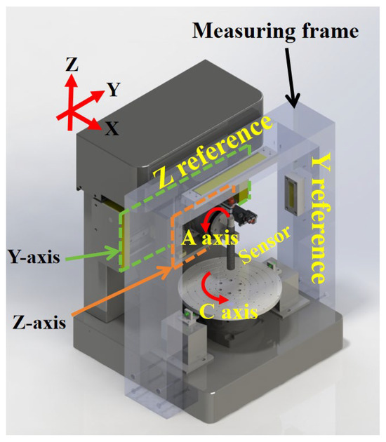
Figure 1.
Structure model of measuring machine.
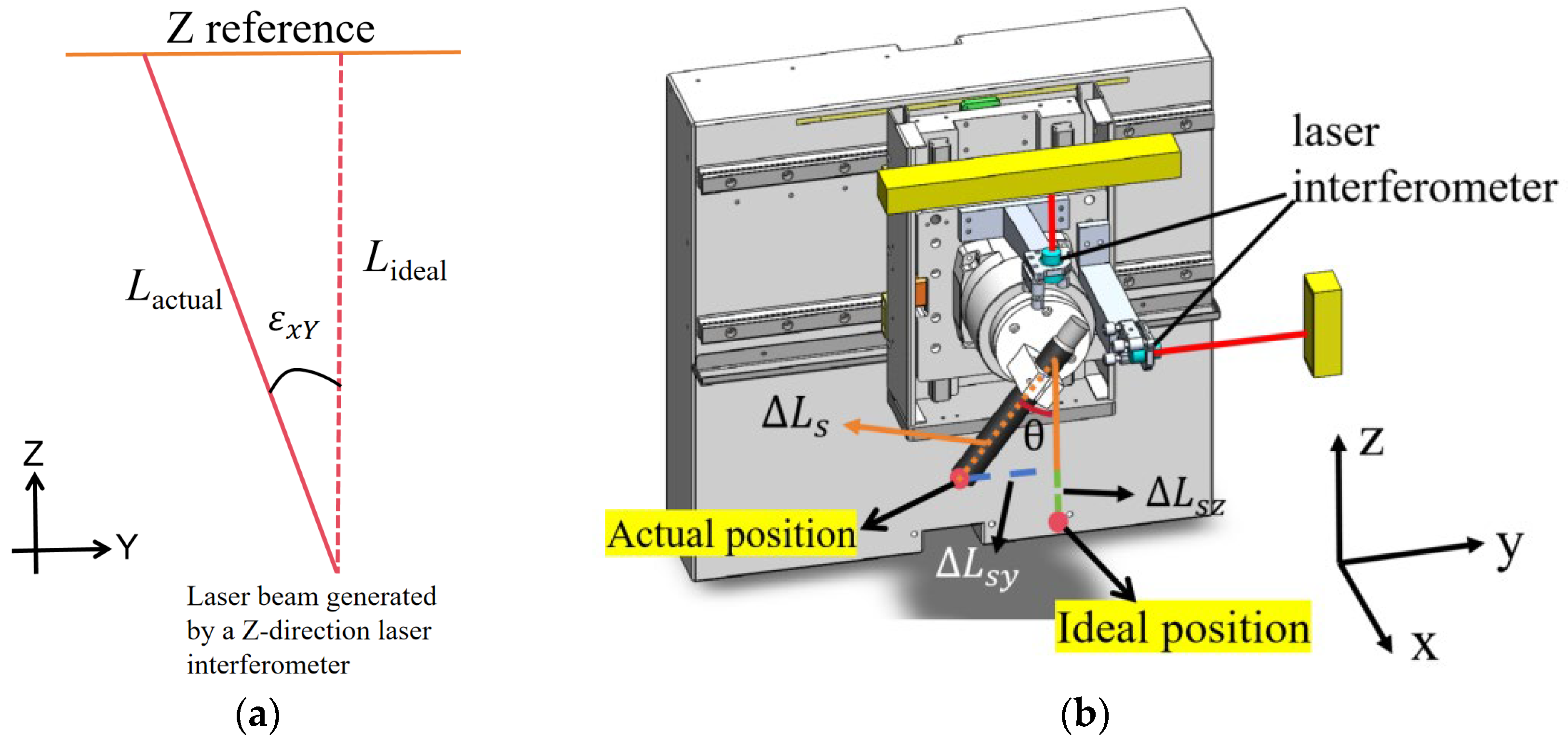
In a traditional CMM, the main reason affecting the measurement uncertainty is the difficulty of simultaneously conforming to the Abbe principle in the measurement direction, which seriously limits the improvement of CMM measurement accuracy. In order to solve this difficulty and avoid the influence of Abbe error on the measurement, the above measurement device is designed, which consists of Y- and Z-laser interferometers with the measurement surface parallel to the Y-axis and Z-axis guide surfaces. By installing mutually perpendicular high-precision mirrors on the measuring frame and adjusting the angle of the two-axis laser interferometer so that the laser beams of the laser interferometer and the axes of the two rotary axes intersect at the center of rotation of the probe, the measurement system of the measuring device is constituted, so that the designed measuring device has an Abbe arm of zero in space.
To analyze the rigid geometry error of the measuring instrument, we assumed that the mirrors were perpendicular and devoid of topographical errors, that the laser scale lines were perpendicular, and that the influence of the guideway motion error was considered separately. The main reason for the positioning error in the measuring machine was the indication error of the laser interferometer. The indication error includes the system error of the laser interferometer and the Abbe error. However, the system error of the laser interferometer is not discussed in this study.
For the linear axis, the straightness motion and angular motion errors are caused by imperfections in the linear guide system [28]. The movement of the Y-axis guide rail produces positioning error ( and Y- and Z-direction straightness errors ( and ), as well as three angular motion errors around the X-, Y-, and Z-axes: , , and . These angular motion errors cause micro-displacement along the other axes. Therefore, the Y-direction positioning error and Z-direction straightness error generated by the movement of the Y-axis guideway cause the Y- and Z-direction laser interferometer signals to have an error of and . For the change in laser interferometer signals caused by angular motion errors, see Figure 2a (taking the effect of angular error on the Z-direction laser interferometer signals as an example). After generating an angular error of , the laser interferometer signal in the Z-direction will generate an error of , where . Through the precision manufacturing of the straight axis, the Angle error does not exceed 1′. Assuming that the Angle error is 1′, the maximum stroke of the Z-axis is 80 mm, and in the Z-direction, the displacement due to the Angle error is 3.38 nm. The resulting error is negligible during the full travel measurement. Therefore, the changes in the laser interferometer signal caused by the geometric error of the Y-axis guideway are mainly due to the positioning error and the Z-direction straightness error . Similarly, the Z-axis guideway produces six geometric errors , , , , , and in the process of movement, which have an impact on the measurement of the main positioning error and straightness error . Because of the structural factors of the measuring machine, the positional errors generated in the X-direction are corrected using the measuring system at a later stage.

Figure 2.
(a) Change caused by angular motion error. (b) Error caused by probe deviating from the ideal direction.
In practice, the probe position may deviate from the ideal position, as shown in Figure 2b. Assuming the angle between the actual probe position and the ideal position is θ, the probe measuring point relative to the intersection of the laser interferometer distance , in the Y-direction, has a deviation value of , where . In the Z-direction the deviation value is , where ). When the A turntable rotates, due to the existence of positioning error, the actual staying position will deviate from the ideal position; the deviation angle is θ, the positioning error is controlled within 1arc sec, the size of is 100 mm, which is calculated in the formula, and the resulting error is very small, which is negligible relative to the full stroke.
The verticality error between the Y-axis and the Z-axis arises from production and installation errors of the guide rail and the Y and Z standard flat crystals. Consequently, the laser lines from the Y and Z laser interferometers are not strictly vertical, leading to verticality and squareness errors of the angle between them. When the mobile platform moves along the Z-direction, a position change in the size occurs in the Y-direction.
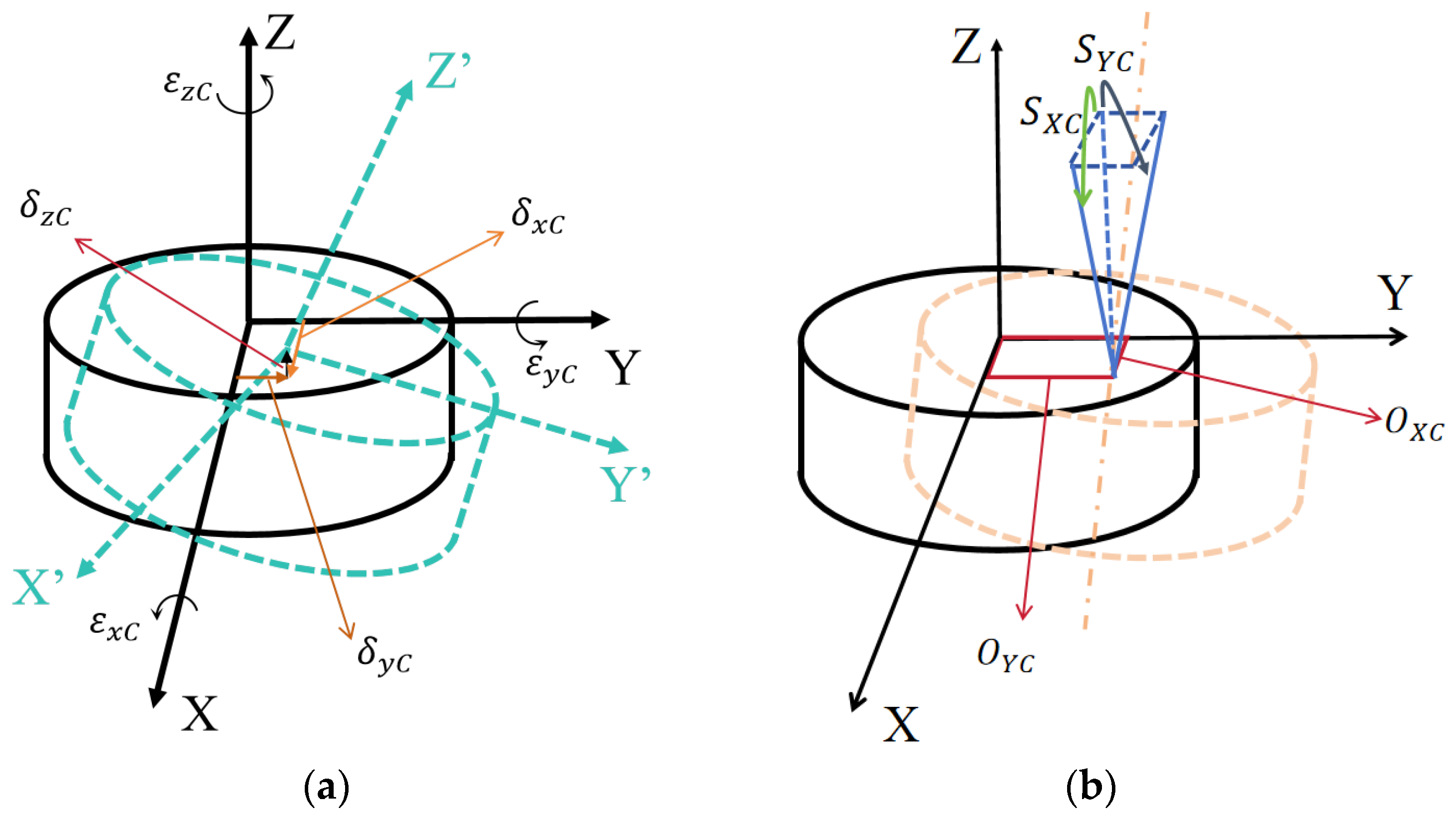
Similar to the linear axis, the rotating axis has six position-dependent geometric errors (PDGEs). The instantaneous error of the rotating axis generates six degrees of freedom, resulting in three position errors (, , and ) and three angle errors (, , and ), as shown in Figure 3a. Three angular errors cause the rotation axis to rotate around the X-, Y-, and Z-axes, and three position errors cause the rotation axis to shift slightly in the X-, Y-, and Z-directions. The absolute representation method was used to define the position-independent geometric errors (PIGEs) of the rotating axis [29] based on the base coordinate system of the platform. For example, considering the C-axis of the rotating axis, each rotating axis contains four PIGEs. The four errors of the rotating shaft from the assembly are two squareness errors ( and ) and two position errors ( and ), as shown in Figure 3b. The value of the two position errors is equal to the position error term when the C-axis rotation angle is 0° and thus can be incorporated into the C-axis error, eliminating the need for separate error matrix calculations. Additionally, the static error matrix between adjacent bodies on a machine tool is a unit matrix. Therefore, the error transformation homogeneous matrix of the C-axis can be represented by Equation (2).
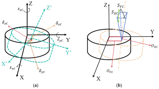
Figure 3.
(a) Six PDGEs in the rotary stage. (b) Four PIGEs in the rotary stage.
Similarly, the error homogeneous transformation matrix of the A-axis can be represented by Equation (3).
On the Y-axis, the Z-axis motion distances are Y and Z. After the A rotary table and C rotary table are rotated by and angles, respectively, the sensor’s signal is L. At this time, the ideal error-free and actual conditions between the probe and the workpiece are measured. The comprehensive error transformation matrix is shown in Equation (4).
where is the actual transformation matrix between the probe and the measured workpiece; is the ideal transformation matrix between the probe and measured workpiece; is the ideal pose transformation matrix between adjacent axes; and is the actual pose transformation matrix between adjacent axes, where j = C, Y, Z, A.
Overall, based on the assumption of a small error and excluding the small amount of second-order and above errors, the components , , and of the comprehensive error model of the measuring machine in the X-, Y-, and Z-directions is obtained as shown in Equations (5)–(7).
3. Geometric Error Weight
Twenty-three error components were considered in the instrument’s conceptual design, as shown in Table 1.

Table 1.
The 23 different errors in the model.
Through analysis of the structural and geometric errors, a spatial volume error model of 23 geometric errors was established by excluding the linear axis angle error, which had minimal influence on the measurement results. The weights of the 23 geometric errors were calculated using the differential solution method. The weight coefficient matrix of the spatial geometric error related to the motion position of the measurement instrument is as follows:
From left to right, Equation (8) includes Y-axis positioning errors, two Y-axis straightness errors, Z-axis positioning errors, two Z-axis straightness errors, six A-axis PDGEs, six C-axis PDGEs and five squareness errors. The described volume error model was used to obtain the corresponding error weight coefficient matrix.
The weight coefficient of each error element in each direction position is defined as follows:
where , , , () represent the weight coefficients of the error component to , , , and . , , and are the volume errors of the measurement points in three directions of the spatial coordinate system. denotes the entire measurement space of the measuring machine. This is expressed as follows:
The physical meaning of the error weight coefficient is the change in the spatial position error caused by the unit variation in the 23 geometric errors in the measurement machine. The greater the weight coefficient W of the error element, the greater the influence of the error element on the spatial positioning accuracy of the machine.
To strengthen the comparative analysis of the data, the error weight was normalized to obtain the error weight coefficient, which is defined as Equation (11):
The basic values of the geometric errors were set to intuitively reflect the influence of various geometric errors on measurement accuracy. The positioning and straightness errors are set to 1 μm; the basic angle error is set to 2 μm/m; and the squareness error is set to 4 μm/m [30]. As presented in Table 2, an error weight analysis under four different measurement conditions was performed with the C-axis as the measured workpiece axis considering the actual measurement process. The four sets of data represent the translation of the two linear axes and the rotation of the two rotating axes for different measurement workpieces. The difference between the four groups is that the A- and C-axes rotate at different angles, while the Y-axis and Z-axis move different distances. The reason for setting different positions for each axis is that in the actual measurement, different types of workpiece contours can be measured by the rotation of the rotating axis and the translation of the linear axis.
Table 2.
Parameter values for error weight analysis.
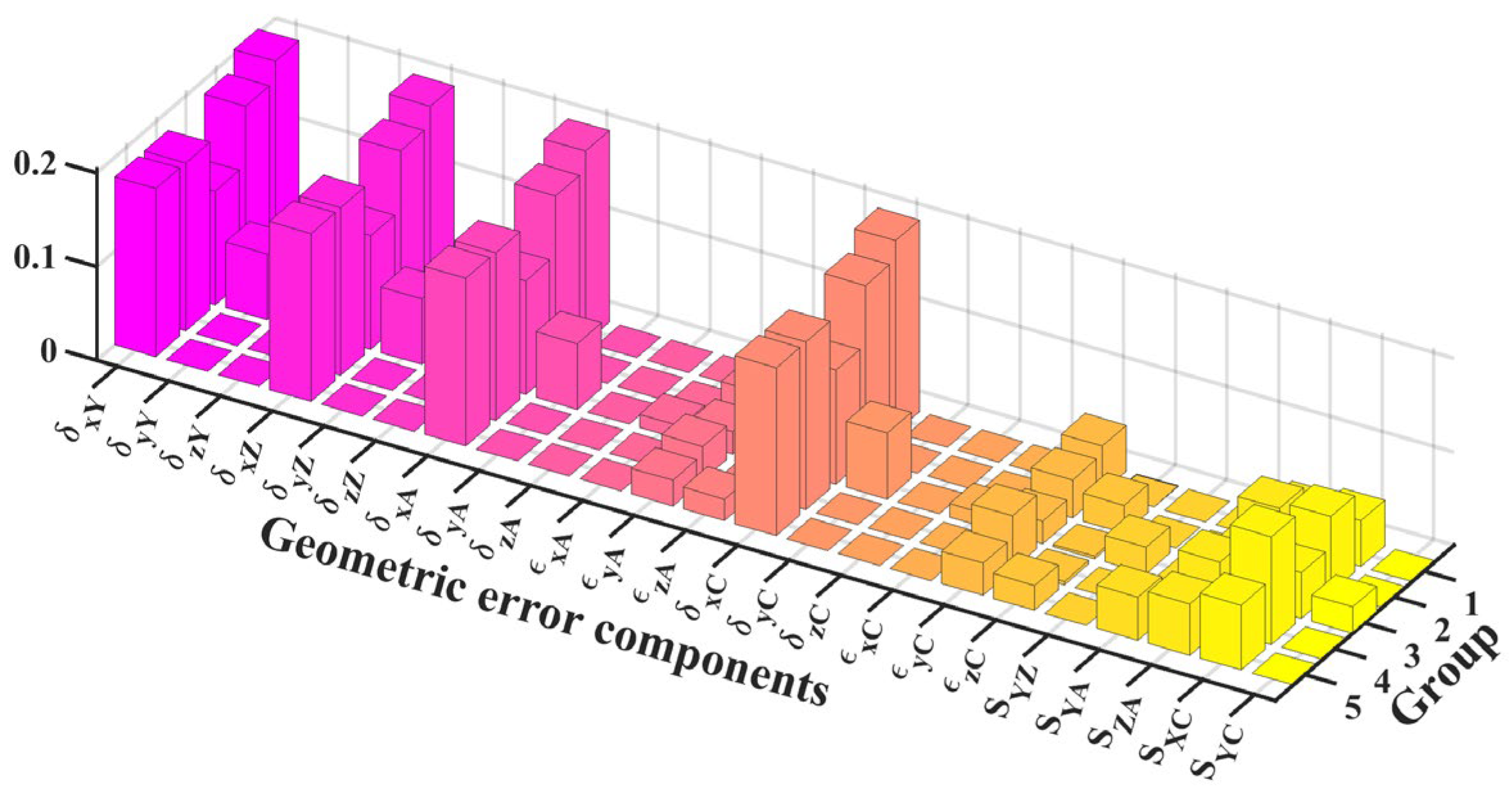
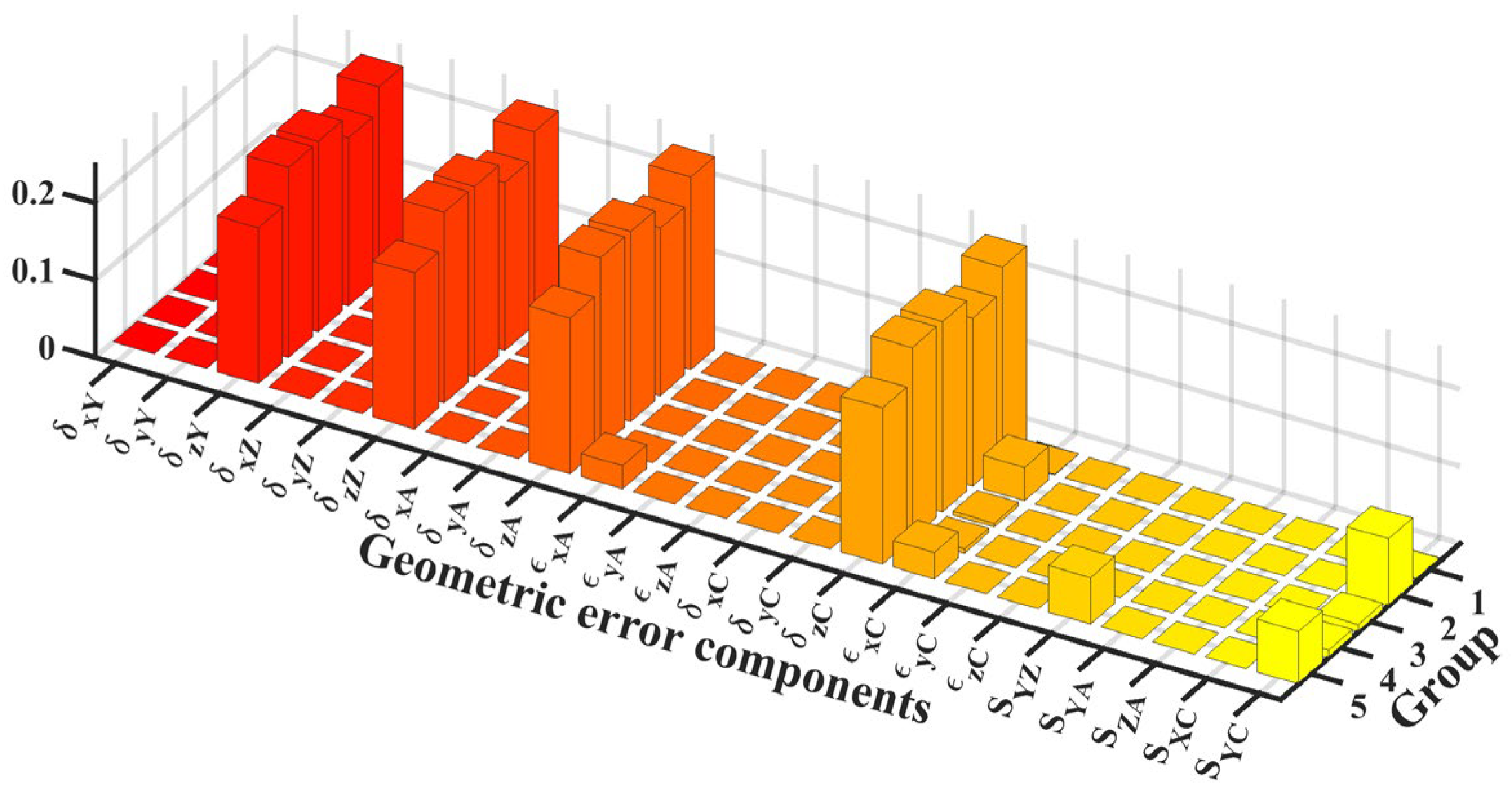
The geometric error weights of the 23 errors in the three directions of the spatial coordinate system and the entire measurement space were calculated using the differential solution method. The results are shown in Figure 4, Figure 5, Figure 6 and Figure 7.

Figure 4.
Error weight analysis for .
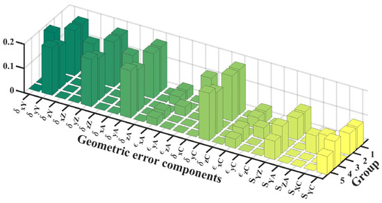
Figure 5.
Error weight analysis for .

Figure 6.
Error weight analysis for .
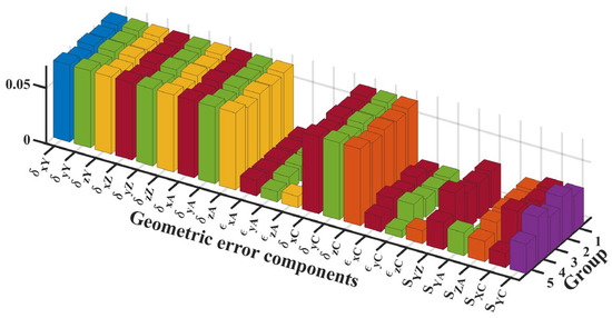
Figure 7.
Error weight analysis for .
Figure 4, Figure 5, Figure 6 and Figure 7 present the error weight analyses of the five groups of positions. The diagram revealed that the position error has a significantly greater impact on volume error than the angle error, and the high-weight error components are the positioning and straightness errors. For the angle error, the influence of the squareness error on the measurement accuracy was significantly higher than that of the angular motion error. The error component with a weight coefficient greater than 0.05 is considered the high-weight error component.
Analyses show that , , , are the key error components of . While the X- and Z-axes’ movement increases error weight owing to error accumulation, it does not constitute a high-weight error. When the C-axis rotates, the weight of , , , , , , , and decreases or increases, and the weight of , , , , , , , and increases or decreases accordingly. This is because the error model established by this method changes the position of the coordinate system after the C-axis is rotated in the reference coordinate system. For example, when the workpiece coordinate system of the C-axis rotates 90° around the Z-axis, the X-axis coincides with the Y-axis of the reference coordinate system while the X-axis coincides with the negative direction of the Y-axis. A-axis rotation will also increase the weight of low-weight errors , , and ; however, they are still not high-weight error components. Similarly, , , , and are the key error components of , while , , , are the key error components of . The rotation of the A-axis affects the weight of the error, but does not affect the dominant position of the high-weight error on the measurement accuracy. , , , , , , , , , , , and are the high-weight errors of .
The geometric error weight is determined using the differential geometric error weight calculation method. The results show that the positioning and straightness errors of each axis significantly influence the measurement accuracy. During the measurement, the motion of the rotation axis increases the weights of some low-weight error components. Although these errors do not become high-weight error components, the weights of the key error components exhibit a smaller reduction. Additionally, the motion of the rotation axis also changes the position of the coordinate system such that some error components change periodically in the one-way error weight analysis; however, it does not affect the comprehensive error model. Owing to the structure of the measuring machine, the probe is always perpendicular to the measured surface, and its tangential position measurement error produces only a negligible second-order error [31]. Therefore, for the comprehensive error, the main high-weight errors are , , , , , , , and .
In the precise design and manufacturing of a measuring machine, attention should be given to the influence of high-weight error components. The geometric error weight analysis results were used for the design and manufacture of the subsequent measuring machines.
4. Experiment
Figure 8 shows the designed large-aperture coordinate precision measurement instrument. The Y- and Z-axes are moved by a linear motor and a ball screw bearing, respectively, and the Y-axis travel is 300 mm and the Z-axis travel is 80 mm. The linear axis also uses a Renishaw RGSZ20-S grating ruler for position feedback. The A- and C-axes consist of a high-precision air-bearing rotary table using an angle encoder (Renishaw RESA30USA) for angular displacement feedback. The probe system was fixed to the A-axis assembly, and the C-axis was used as the measured workpiece axis. The measurement framework used a quDIS displacement measurement interferometer to accurately match the standard ruler feedback probe position. The measurement instrument specifications are shown in Table 3. The results of the geometric error weighting analysis were applied to the accuracy design and manufacture of large-aperture coordinate precision measurement instruments, Subsequently, performance tests were conducted.
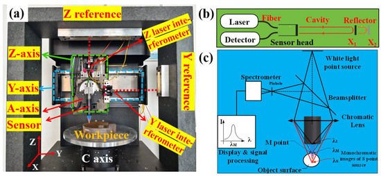
Figure 8.
Design of large-aperture coordinate precision measurement instrument. (a) Setup of the instrument. (b) Principle of the laser interferometer. (c) Principle of the sensor.
Table 3.
The specifications and main error requirements of measuring machine.
4.1. Effects of Static Noise
In high-precision measurements, the external environmental effect is crucial for the measurement data. In dynamic measurements, the influence of external vibrations or the environment leads to oscillation of the sensor return data. Consequently, the data reliability of the equipment in dynamic measurement is reduced, resulting in poor repeatability. Therefore, the static noise data of the measurement system are collected by the probe and used to analyze the effect of static noise on the measurement accuracy.
The noise observed in the measured data originates from the system’s operation factors, including temperature, humidity, pressure gradient, and proportion integration differentiation control. Owing to experimental conditions, the respective frequencies of these noises remain determined; therefore, only qualitative descriptions are available, with pending quantitative analysis. Figure 9a shows the static noise data collected by the measuring head at a sampling frequency of 100 HZ for 10 s, showing its stability within 88 nm. Figure 9b shows that the amplitude of the laser interferometer’s inherent noise is within 10 nm and tends to stabilize. Overall, the level of readout noise during system operation was stable and very little, both on the sub-micron scale.
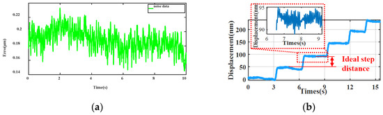
Figure 9.
Static noise test. (a) Noise measurement of the sensor. (b) Noise measurement of the laser interferometer.
4.2. High-Weight Error Measurement and Compensation
The straightness error is a position-dependent geometric error, while the magnitude of the error varies with changes in the coordinate position. Based on the weight analysis of the previous section, the positioning error and the straightness motion error are the main errors affecting the measurement accuracy, necessitating accurate measurement and compensation.
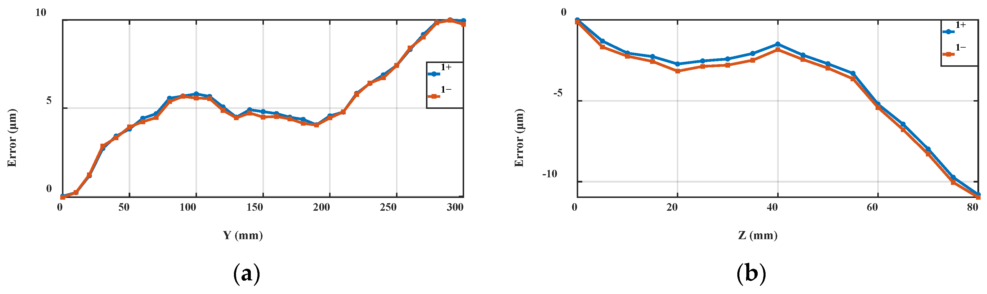
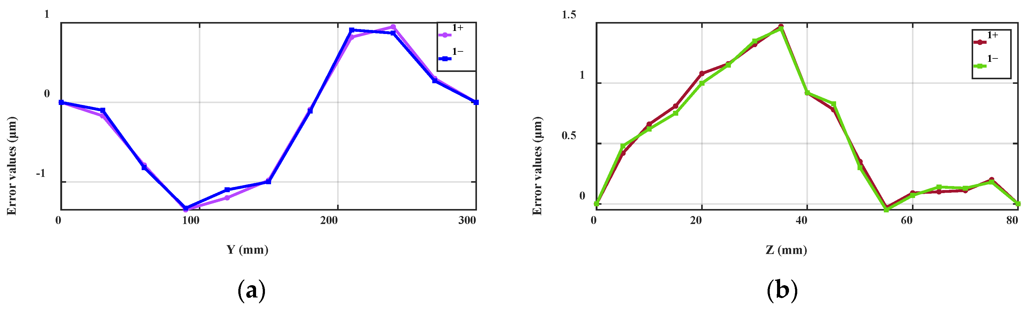
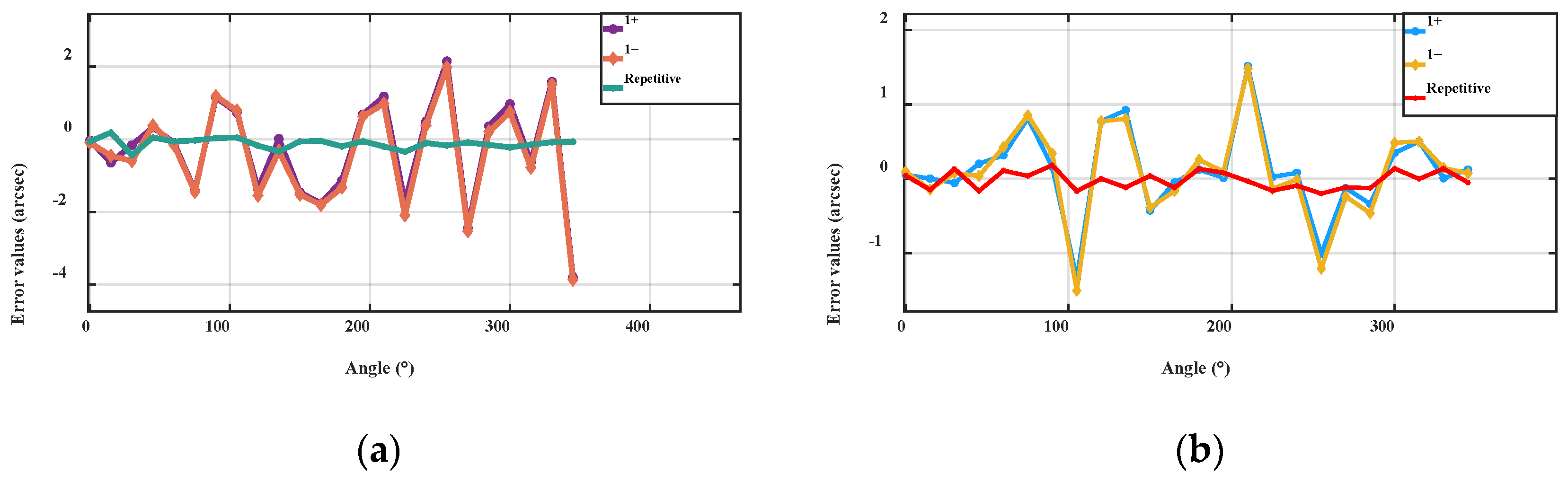
The linear guide adopts the Renishaw RGSZ20-S grating ruler as the position reference, with a linearity of ±3 μm/m. The positioning and straightness errors of the linear axis were obtained by measuring the Y- and Z-axes using a Renishaw XK-10 laser interferometer, as shown in Figure 10. The measurement results are shown in Figure 11 and Figure 12; 1+ indicates traveling in the positive direction forwards, 1− indicates traveling in the opposite direction forwards, and the number indicates the number of repetitions. The Y-axis positioning accuracy is 10.1 μm, while the Z-axis straightness error is 2.3 μm per 300 mm. The Z-axis positioning accuracy is 11 μm, and the Y-axis straightness error is 1.5 μm per 80 mm.
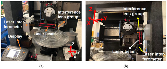
Figure 10.
Positioning accuracy and straightness measurement of Y-axis (a) and Z-axis (b).

Figure 11.
Positioning accuracy of Y-axis (a) and Z-axis (b).
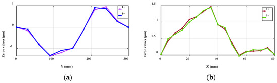
Figure 12.
Straightness error on the Y-axis (a) and Z-axis (b).
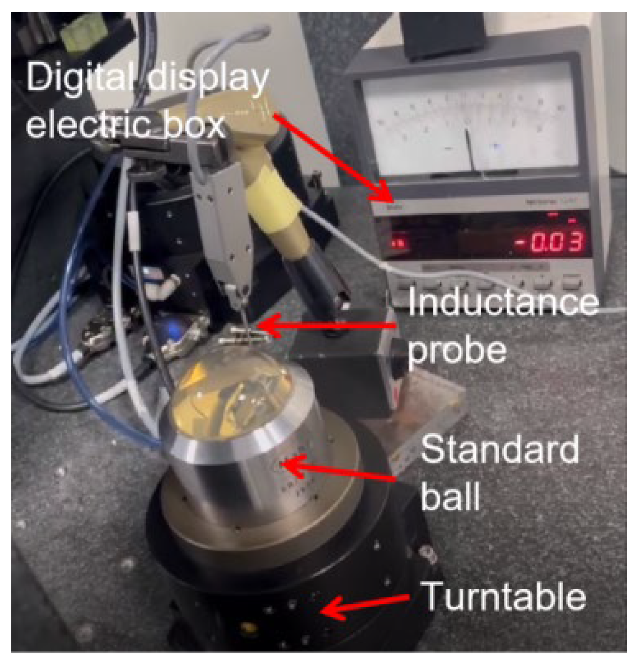
The rotary table is a self-developed high-precision air-bearing model [32,33]. The positioning accuracy and repeatability of the rotary table were tested using a 24-plane prism with collimator. The results are shown in Figure 13. The positioning accuracy of the A rotary table is ±2.52 arc sec and the repeatability is about ±0.44 arc sec, and the positioning accuracy of the C rotary table is ±1.69 arc sec and the repeatability is about ±0.51 arc sec. The axial and radial runouts of the rotary table were tested using a standard sphere with a roundness of 50 nm and an inductive micrometer. As shown in Figure 14, the rotation of the tested air-bearing rotary table is controlled to 360°. The radial runout error of the air-bearing rotary table and the roundness error of the standard sphere were separated using a reverse method [34]. The radial runout error of the air-bearing rotary table was obtained by subtracting the positive and negative data and averaging them. The axial runout error of the air-bearing rotary table was obtained using the error separation technique of mathematical statistics [35]. The radial runout of the A-axis air-bearing rotary table was greater than 100 nm, while the axial runout was greater than 75 nm. Similarly, the radial runout of the C-axis air-bearing rotary table was greater than 100 nm and the axial runout was greater than 50 nm, which meets the needs of the experiment.
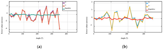
Figure 13.
Repeated positioning accuracy of rotary table A (a) and rotary table C (b).

Figure 14.
Jump test of air-bearing rotary table.
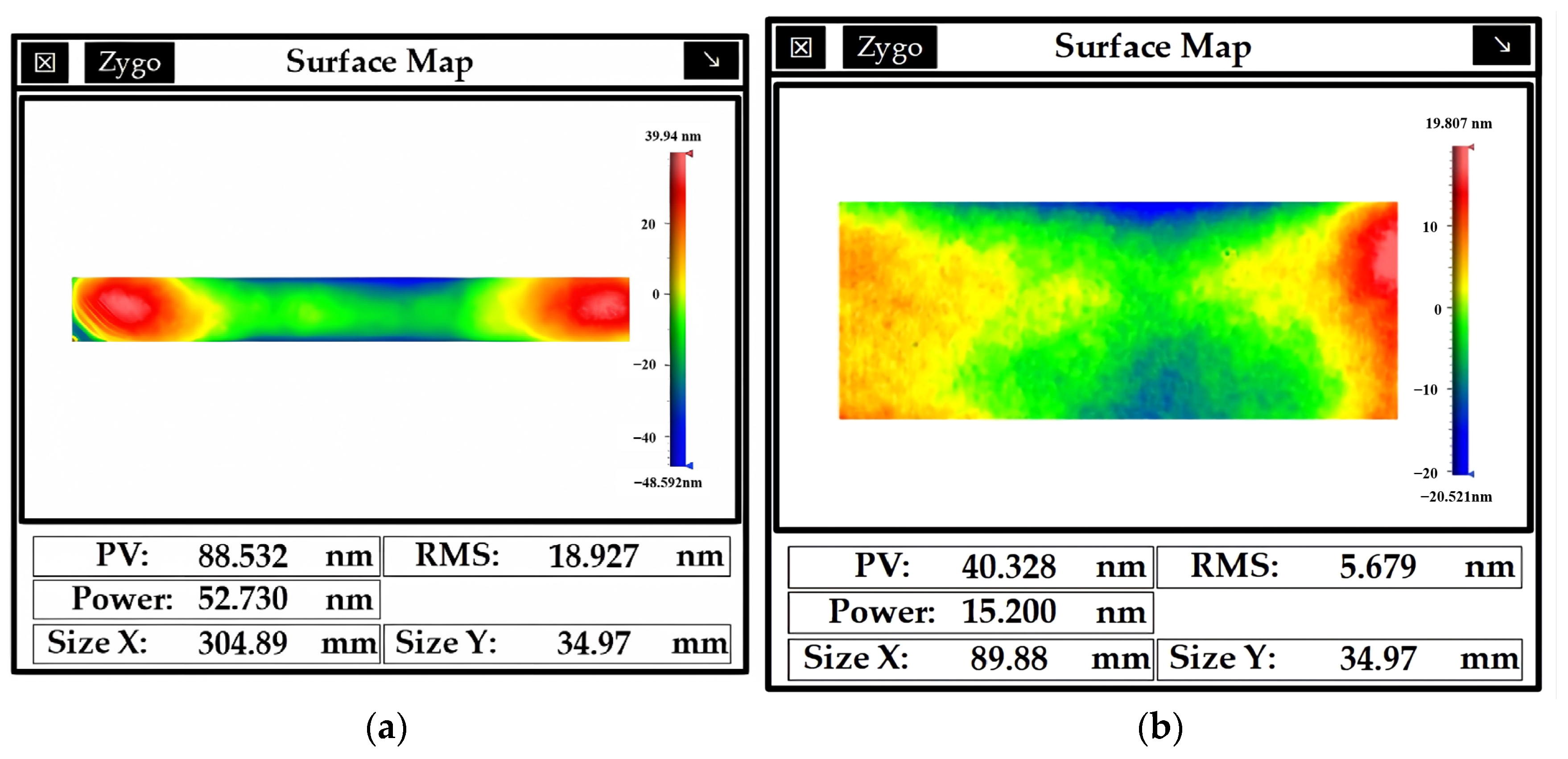
To verify the compensation ability of the measuring frame, a picometer-level precision laser interferometer (quDIS) was used for high-precision positioning of the measuring machine. A standard flat ruler was also used to compensate for the straightness error in real-time. The accuracies of the surface shapes of the standard flat rulers are shown in Figure 15.

Figure 15.
Accuracy of the surface shape of standard flat rulers: (a) Standard flat rulers in the Y-direction, (b) Standard flat rulers in the Z-direction.
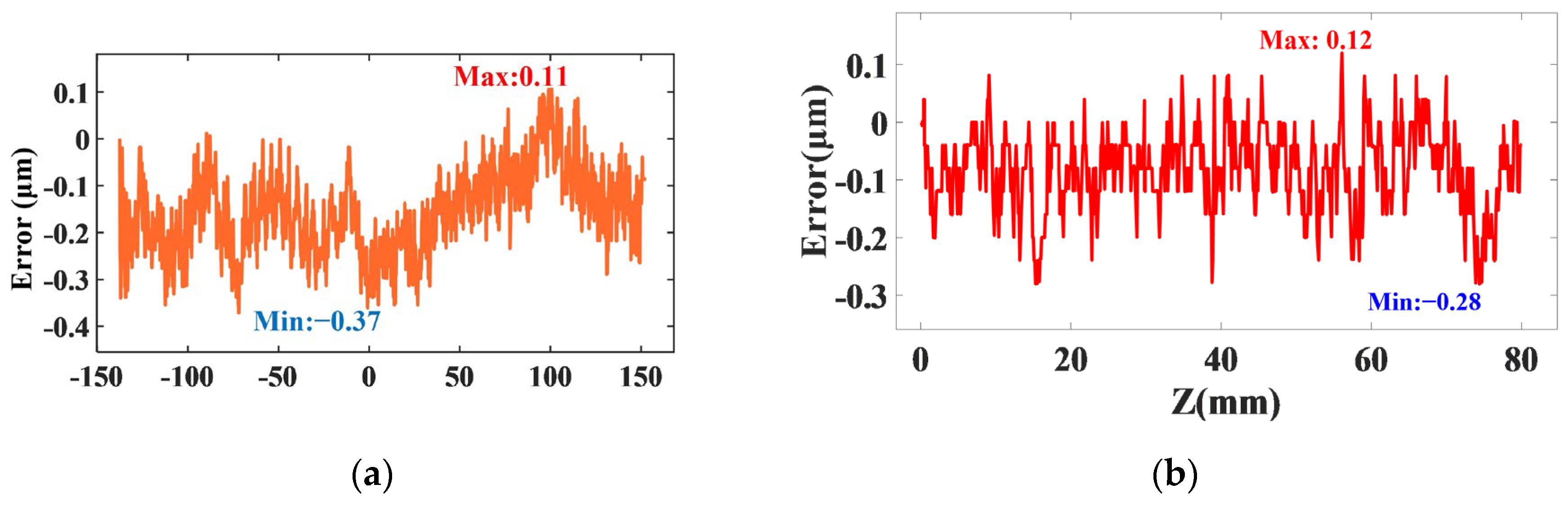
The measurement framework utilizes a quDIS and a high-precision ruler to compensate for the positioning accuracy and straightness of the linear axis. The theoretical positioning accuracy of the quDIS reaches 0.2 nm/mm and the working distance is 20–400 mm. During the Y-axis movement, the workbench produces a positioning error in the Y-direction and a straightness motion error in the Z-direction, resulting in micro-displacements. The Y-axis position is continuously read in real time by the quDIS sensor head in the Y-direction, and the value displayed by the quDIS is taken as the actual position of the Y-axis. The quDIS provides high-precision positioning and can accurately obtain the motion position of the Y-axis, thereby compensating for the error caused by inaccurate positioning on the straight axis. It also detects and compensates for Y-axis straightness errors in the Z-direction with a Z-direction sensor probe. Similarly, the error caused by the Z-axis movement was read and compensated by the measurement system in real time. The straightness error data were measured using the quDIS, and the data were fitted using the least-squares method, as shown in Figure 16. The Y-axis Z-direction straightness is reduced from 2.3 μm per 300 mm to 0.48 μm per 300 mm, and the Z-axis Y-direction straightness is reduced from 1.5 μm per 80 mm to 0.40 μm per 80 mm.
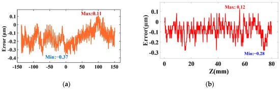
Figure 16.
Straightness error on the Y-axis (a) and Z-axis (b) after compensation.
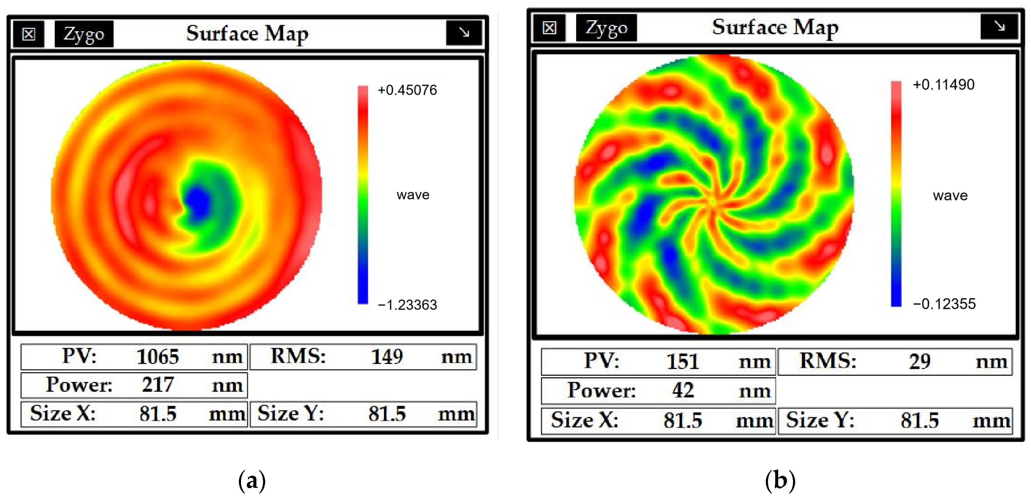
In order to verify the accuracy of the measuring system, a high-precision flat mirror with a diameter of 82 mm was measured. Figure 17a shows the original measurement result of the measuring instrument. After compensating for geometric errors of high weights, the results obtained are shown in Figure 17b. As the result of compensation, the compensation effect is obvious. However, the result of the compensated pattern shows an eddy current pattern. It may be due to a small displacement in the measurement process, or poor alignment, inaccurate system calibration, or other reasons, which need to be further explored.

Figure 17.
High-precision flat mirror measurement results: (a) before compensation, (b) after compensation.
The accuracy of each high-weighting error of the measuring instrument is presented in Table 4 and Table 5. The results of the preliminary experiments proved that, by controlling the high-weighting errors, the measuring platform can effectively realize high-precision positioning and real-time compensation of straightness, and the designed high-precision large-diameter measuring machine has high accuracy and effectiveness.
Table 4.
The accuracy of each high-weight error of the linear axis.
Table 5.
The accuracy of each high-weight error of the turntables.
5. Conclusions
In this study, the volume error modeling of a large-aperture coordinate precision measurement instrument was investigated, and its geometric error weight was analyzed to guide the precision design and manufacture of the measuring instrument. According to the multi-body theory and the small angle hypothesis, a geometric error model containing 23 error components was established. Additionally, a differential-geometric error weight analysis method was proposed to analyze the geometric error weights of 23 error components in the volumetric errors , , , and . The error weight coefficients of each geometric error component were obtained, which identified the main geometric errors affecting the accuracy of the measuring instrument. The results show that:
- (1)
- The error weight proportions of the angle and verticality errors are very small, and can be excluded compared with the positioning and straightness errors. The different measurement points under the motion of the rotating and translational axes did not affect the key error components of the volume error;
- (2)
- The key error components of , , , and were obtained. Additionally, the motion of the rotation axis causes the position of the coordinate system to change, resulting in periodic variation in certain error components in the error weighting analysis of the unidirectional error model but essentially having no effect on the composite error model. During the measurement, the movement of the rotary axis increases the weight of certain low-weight error components. Although they still do not become high-weighted error components, this results in a small reduction in the weights of the critical error components, making it challenging to improve the accuracy of the measuring machine.
The results of the geometric error weight analysis are effectively used in the precision design and manufacture of large-aperture coordinate precision measurement instruments. The preliminary experiment of high-weight error measurement and compensation proves the effectiveness of the real-time compensation of the measurement framework and the high precision and effectiveness of the designed large-aperture coordinate precision measurement instrument, The measures taken to compensate for the different errors are shown in Table 6.
Table 6.
Measures taken to compensate for high-weight errors.
In future work, we will use the measuring instrument to perform measurement experiments, and the coupling between different errors of different axes of the measuring machine will be further studied to improve the method of compensating only for the high-weight errors, improving the measurement accuracy of the measuring machine.
Author Contributions
Conceptualization, S.L., H.K., T.L. and J.L.; methodology, S.L., T.L. and J.L.; validation, S.L., T.L. and J.L.; formal analysis, S.L., T.L. and J.L.; investigation, S.L., T.L., Y.Z. (Yiang Zhang) and Y.Z. (Yufang Zhou); resources, S.L. and T.L.; data curation, S.L.; writing—original draft preparation, S.L.; writing—review and editing, S.L., T.L. and J.L.; visualization, S.L.; supervision, Z.L., T.L. and J.L.; funding acquisition, T.L. and J.L. All authors have read and agreed to the published version of the manuscript.
Funding
The National Natural Science Foundation of China (Nos. 52205505, No.52375473), the science and technology innovation Program of Hunan Province (2024RC3235), and National University of Defense Technology Research Program (ZK22-12).
Institutional Review Board Statement
Not applicable.
Informed Consent Statement
Not applicable.
Data Availability Statement
The data presented in this study are available upon request from the corresponding author. The data are not publicly available because they are part of an ongoing study.
Acknowledgments
Thanks to the collaborators for their support and help to the authors during the research and paper writing process, as well as the technical support of the staff of Hunan Advanced Research Institute.
Conflicts of Interest
The authors declare no conflicts of interest.
References
- Kumar, S.; Tong, Z.; Jiang, X. Advances in the design and manufacturing of novel freeform optics. Int. J. Extrem. Manuf. 2022, 4, 032004. [Google Scholar] [CrossRef]
- Acko, B.; McCarthy, M.; Haertig, F.; Buchmeister, B. Standards for testing freeform measurement capability of optical and tactile coordinate measuring machines. Meas. Sci. Technol. 2012, 23, 094013. [Google Scholar] [CrossRef]
- Chen, S.; Xue, S.; Zhai, D.; Tie, G. Measurement of Freeform Optical Surfaces: Trade-Off between Accuracy and Dynamic Range. Laser Photonics Rev. 2020, 14, 1900365. [Google Scholar] [CrossRef]
- Zhang, Z.; Jiang, F.; Luo, M.; Wu, B.; Zhang, D.; Tang, K. Geometric error measuring, modeling, and compensation for CNC machine tools: A review. Chin. J. Aeronaut. 2024, 37, 163–198. [Google Scholar] [CrossRef]
- Han, J.; Wang, L.; Ma, F.; Ge, Z.; Wang, D.; Li, X. Sensitivity analysis of geometric error for a novel slide grinder based on improved Sobol method and its application. Int. J. Adv. Manuf. Technol. 2022, 121, 6661–6684. [Google Scholar] [CrossRef]
- Cheng, Q.; Sun, B.; Liu, Z.; Li, J.; Dong, X.; Gu, P. Key Geometric Error Extraction of Machine Tool Based on Extended Fourier Amplitude Sensitivity Test Method. Int. J. Adv. Manuf. Technol. 2017, 90, 3369–3385. [Google Scholar] [CrossRef]
- Chen, G.; Ding, S.; Xu, G. Novel method for identifying sensitive geometric errors of CNC machine tools oriented to cylindricity in flank milling. J. Manuf. Process. 2024, 126, 370–381. [Google Scholar] [CrossRef]
- Wu, H.; Zheng, H.; Li, X.; Wang, W.; Xiang, X.; Meng, X. A Geometric Accuracy Analysis and Tolerance Robust Design Approach for a Vertical Machining Center Based on the Reliability Theory. Measurement 2020, 161, 107809. [Google Scholar] [CrossRef]
- Zhang, X.; Zhang, Y.; Pandey, M.D. Global Sensitivity Analysis of a CNC Machine Tool: Application of MDRM. Int. J. Adv. Manuf. Technol. 2015, 81, 159–169. [Google Scholar] [CrossRef]
- Cai, L.; Zhang, Z.; Cheng, Q.; Liu, Z.; Gu, P.; Qi, Y. An Approach to Optimize the Machining Accuracy Retainability of Multi-Axis NC Machine Tool Based on Robust Design. Precis. Eng. 2016, 43, 370–386. [Google Scholar] [CrossRef]
- Li, G.; Wu, C.; Xu, K.; Ran, Q.; Cao, B. Pivotal Errors Identification of the Face Gear Worm Grinding Machine Tool with a Piecewise Sensitivity Analysis. Mech. Mach. Theory 2023, 181, 105206. [Google Scholar] [CrossRef]
- Jiang, X.; Cui, Z.; Wang, L.; Liu, C.; Li, M.; Liu, J.; Du, Y. Critical Geometric Errors Identification of a Five-Axis Machine Tool Based on Global Quantitative Sensitivity Analysis. Int. J. Adv. Manuf. Technol. 2022, 119, 3717–3727. [Google Scholar] [CrossRef]
- Fu, G.; Gong, H.; Fu, J.; Gao, H.; Deng, X. Geometric Error Contribution Modeling and Sensitivity Evaluating for Each Axis of Five-Axis Machine Tools Based on POE Theory and Transforming Differential Changes between Coordinate Frames. Int. J. Mach. Tools Manuf. 2019, 147, 10103455. [Google Scholar] [CrossRef]
- Lai, T.; Liu, J.; Chen, F.; Li, Z.; Guan, C.; Li, H.; Xu, C.; Hu, H.; Dai, Y.; Chen, S.; et al. Allocation of Geometrical Errors for Developing Precision Measurement Machine. J. Intell. Manuf. 2024, 1–23. [Google Scholar] [CrossRef]
- Liu, C.S.; Hsu, H.C.; Lin, Y.X. Design of a Six-Degree-of-Freedom Geometric Errors Measurement System for a Rotary Axis of a Machine Tool. Opt. Lasers Eng. 2020, 127, 105949. [Google Scholar] [CrossRef]
- Hu, P.; Zhang, J.; Ma, Q. Analysis of Slider Motion Error on 3-PUU Parallel Coordinate Measuring Machining. J. Mech. Eng. 2015, 51, 45–50. [Google Scholar] [CrossRef]
- Liu, H.; Xiang, H.; Chen, J.; Yang, R. Measurement and Compensation of Machine Tool Geometry Error Based on Abbe Principle. Int. J. Adv. Manuf. Technol. 2018, 98, 2769–2774. [Google Scholar] [CrossRef]
- Huang, Y.B.; Fan, K.C.; Lou, Z.F.; Sun, W. A Novel Modeling of Volumetric Errors of Three-Axis Machine Tools Based on Abbe and Bryan Principles. Int. J. Mach. Tools Manuf. 2020, 151, 103527. [Google Scholar] [CrossRef]
- Chen, G.; Zhang, L.; Wang, X.; Wang, C.; Xiang, H.; Tong, G.; Zhao, D. Modeling Method of CNC Tooling Volumetric Error under Consideration of Abbé Error. Int. J. Adv. Manuf. Technol. 2022, 119, 7875–7887. [Google Scholar] [CrossRef]
- He, Y.X.; Lin, R.W.; Li, R.J.; Li, J.; Cheng, Z.Y.; Pan, Q.S.; Huang, Q.X.; Fan, K.C. Nanopositioning X–Y Stage with an Embedded Six-DOF Error Compensation System Based on Abbe and Bryan Principles. Measurement 2024, 227, 114218. [Google Scholar] [CrossRef]
- Huang, Q.; Wu, K.; Wang, C.; Li, R.; Fan, K.C.; Fei, Y. Development of an Abbe Error Free Micro Coordinate Measuring Machine. Appl. Sci. 2016, 6, 97. [Google Scholar] [CrossRef]
- Henselmans, R.; Cacace, L.A.; Kramer, G.F.Y.; Rosielle, P.C.J.N.; Steinbuch, M. The NanoMeFOS Non-Contact Measurement Machine for Freeform Optics. Precis. Eng. 2011, 35, 607–624. [Google Scholar] [CrossRef]
- Kondo, Y.; Hirai, A.; Youichi, B. Two-point diameter calibration of a sphere using a micro-coordinate measuring machine at NMIJ. Metrologia 2022, 59, 024005. [Google Scholar] [CrossRef]
- Lewis, A.; Oldfield, S.; Peggs, G.N. The NPL small CMM—3-D measurement of small features. In WIT Transactions on Engineering Sciences; WIT Press: Billerica, MA, USA, 2001. [Google Scholar]
- Schmidt, I.; Hausotte, T.; Gerhardt, U.; Manske, E.; Jäger, G. Investigations and calculations into decreasing the uncertainty of a nanopositioning and nanomeasuring machine (NPM-Machine). Meas. Sci. Technol. 2007, 18, 482–486. [Google Scholar] [CrossRef]
- Jäger, G.; Manske, E.; Hausotte, T.; Büchner, H.J. The metrological basis and operation of nanopositioning and nanomeasuring machine NMM-1. Metrologische Grundlagen und Wirkungsweise der Nanopositionier- und Messmaschine NMM-1. TM Tech. Mess. 2009, 76, 227–234. [Google Scholar] [CrossRef]
- Mussatayev, M.; Huang, M.; Beshleyev, S. Thermal influences as an uncertainty contributor of the coordinate measuring machine (CMM). Int. J. Adv. Manuf. Technol. 2020, 111, 537–547. [Google Scholar] [CrossRef]
- ISO 230-1; Test Code for Machine Tools: Part 1: Geometric Accuracy of Machines Operating Under No-Load or Finishing Conditions. ISO: Geneva, Switzerland, 2020.
- Fan, Y.; Fan, K.C.; Huang, Y. Modeling and compensation of enhanced volumetric error of machine tools containing crosstalk errors. Precis. Eng. 2024, 86, 252–264. [Google Scholar] [CrossRef]
- Tian, W.; Gao, W.; Chang, W.; Nie, Y. Error Modeling and Sensitivity Analysis of a Five-Axis Machine Tool. Math. Probl. Eng. 2014, 201, 745250. [Google Scholar] [CrossRef]
- Henselmans, R.; Cacace, L.; Kramer, G.; Rosielle, N.; Steinbuch, M. Nanometer level freeform surface measurements with the nanomefos non-contact measurement machine. In Proceedings of the Optical Manufacturing and Testing VIII, San Diego, CA, USA, 4–5 August 2009. [Google Scholar]
- Xu, H.; Sun, Z.; Dai, Y.; Guan, C.; Hu, H. In situ measurement and reconstruction technology of cylindrical shape of high-precision mandrel. Micromachines 2023, 14, 1240. [Google Scholar] [CrossRef]
- Xu, H.; Sun, Z.; Dai, Y.; Guan, C.; Hu, H.; Wang, Y. In situ measurement of spindle radial error for ultra-precision machining based on three-point method. Micromachines 2023, 14, 653. [Google Scholar] [CrossRef]
- Castro, H.F.F. A method for evaluating spindle rotation errors of machine tools using a laser interferometer. Measurement 2008, 41, 526–537. [Google Scholar] [CrossRef]
- Marsh, E.; Couey, J.; Vallance, R. Nanometer-level comparison of three spindle error motion separation techniques. J. Manuf. Sci. Eng. 2006, 128, 180–187. [Google Scholar] [CrossRef]


Disclaimer/Publisher’s Note: The statements, opinions and data contained in all publications are solely those of the individual author(s) and contributor(s) and not of MDPI and/or the editor(s). MDPI and/or the editor(s) disclaim responsibility for any injury to people or property resulting from any ideas, methods, instructions or products referred to in the content. |
© 2024 by the authors. Licensee MDPI, Basel, Switzerland. This article is an open access article distributed under the terms and conditions of the Creative Commons Attribution (CC BY) license (https://creativecommons.org/licenses/by/4.0/).