Abstract
The development of automation and intelligence in geological core drilling is not yet mature. The selection and improvement of drilling parameters rely mainly on experience, and adjustments are often made after drilling by evaluating the core, which introduces a lag and reduces the drilling efficiency. Therefore, this study first establishes a geological core drilling experiment platform to collect drilling data. Through the constructed geological core drilling experimental platform, the practical data at the drill bit can be directly obtained, solving the problem of the data from the surface equipment in the practical drilling differing from the practical data. Second, the back propagation (BP) algorithm is used to perform the ROP prediction, with weight on bit (WOB), torque (TOR), flow rate (Q), and rotation speed (RPM) as input parameters, and rate of penetration (ROP) as the output. Subsequently, correlation analysis is used to perform the feature parameter optimization, and the effects of bit wear and bit cutting depth on the experiment are considered. Finally, comparison with algorithms such as ridge regression, SVM and KNN shows that the ROP prediction model using the BP neural network has the highest prediction accuracy of 94.1%. The results provide a reference for ROP prediction and the automation of geological core drilling rigs.
1. Introduction
Geological core drilling is the most direct and effective technique for geological surveys and mineral exploration [1]. In recent years, this has been combined with rapidly developing artificial intelligence technology to improve its level of intelligence. In oil drilling engineering, there are already examples where artificial intelligence algorithms have been combined with existing drilling models to improve drilling efficiency [2,3,4]. Rommetveit and his team [5] developed an automatic drilling monitoring system based on surface and downhole data, called “Drilltronics”. The system focuses on optimizing the drilling pressure and rotational speed. By thoroughly analyzing key factors such as weight on bit and torque during the drilling process, it has successfully improved the mechanical ROP. In practical applications, it has been found that the system can increase the mechanical ROP by 15% to 30%. Additionally, Iversen et al. [6], based on a precise analysis of field measurement data, successfully developed a drilling parameter optimization system. The system utilizes the analysis of factors such as weight on bit and torque on the mechanical ROP, adjusting these parameters to ensure that they remain within the optimal range, thus achieving real-time optimization of the mechanical ROP. C. Gan et al. [7], addressing the characteristics of incompleteness, coupling, and strong nonlinearity of data during the drilling process, established a drilling speed prediction model using an improved particle swarm optimization algorithm to optimize the radial basis function neural network. This provides an important means for intelligent optimization control in complex formation drilling. Chiranth Hegde et al. [8] proposed using data-driven models to achieve optimization of the drilling mechanical speed and the selection of optimal drilling parameters. Experimental results show that applying a random search algorithm can overcome the feedback delay of data in the computation process of conventional models, thereby increasing the mechanical ROP by an average of 30%. Their team also introduced six mechanistic and machine learning modeling methods to establish drilling speed models and used data from the drilling processes of more than ten different formations to test the accuracy of the models. The research results indicate that machine learning methods have higher drilling speed prediction accuracies. Currently, artificial intelligence algorithms have significant advantages in solving complex multiparameter problems. In geological core drilling, by establishing a complex network of relationships among various drilling parameters, it is possible to achieve accurate prediction and optimization of the mechanical ROP, thereby improving drilling efficiency. However, due to the more complex formation conditions targeted by geological core drilling and the resulting lower economic benefits, there has not been significant application of these methods in this field.
The back propagation (BP) neural network is one of the most well-studied neural network algorithms [9], being known for its excellent self-learning, adaptability, robustness, and generalization capabilities. It has received extensive research attention and been applied in many engineering fields. Hazbeh et al. predicted the ROP using AI hybrid models on the directional stage of Kaboud oil-field well #7 [10]. Lawal A I used ant–lion optimization of artificial neural networks for drilling speed prediction [11]. Su K proposed a drilling ROP prediction model that optimizes the weights of the BP neural network by the Improved Chaotic Whale Optimization Algorithm (ICWOA), which improves the accuracy of the drilling speed prediction [12].
The application of machine learning methods for ROP prediction in oil drilling has become quite mature. However, in the field of geological core drilling, ROP prediction still relies on constructing linear models for solutions. The deep geological drilling process involves complex geomechanical environments characterized by high pressure, high temperature, high hardness, and severe disturbance, leading to pronounced issues of nonlinearity, strong coupling, and significant interference. The commonly used impregnated diamond-bit technology differs in its operational parameters and rock-breaking mechanisms compared with those of the PDC and roller-cone bits typically used in oil drilling. Furthermore, data on parameters such as the WOB and TOR in core drilling are collected by surface drilling rig equipment, which differ from the actual signals at the bit. Therefore, the existing advanced ROP prediction models based on drilling engineering parameters do not fully apply to geological core drilling and require further validation. This study focuses on geological core drilling by establishing a micro-drilling experimental platform to obtain practical drilling parameters such as the WOB and torque at the bit during core drilling [13]. The practical drilling parameters will be used as training data for ROP prediction. Through machine learning techniques to explore the relationship between input and output layers, a regression model is established that links drilling parameters to drilling speed.
2. Methods
2.1. BP Neural Network Model
In the practical applications of artificial neural networks, the majority of neural network models use BP networks and their variations, which are also the core part of feed forward networks, embodying the essence of artificial neural networks. The classic topology of a BP neural network is shown in Figure 1.
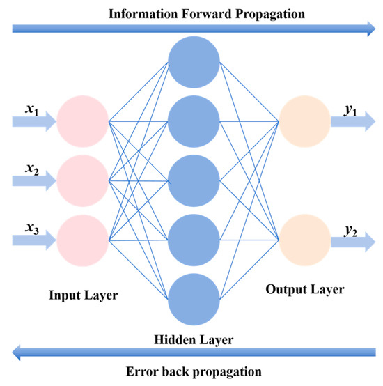
Figure 1.
Topology of a classical BP neural network.
As shown in Figure 1, the BP neural network usually includes an input layer, an output layer, and hidden layers. The BP neural network model is divided into two parts: information forward propagation and error back propagation [2,14].
2.1.1. Forward Propagation Input
First, through the input layer provided by the training samples, the output of each neuron can be calculated. The specific formula is shown in Equation (1).
Here, is the sigmoid activation function; is the network weight from unit i of the previous layer to unit j of this layer; is the output of unit i of the previous layer; and is the bias of the unit, which can change the activity of the unit. The computation for each neuron is a linear combination of its inputs.
2.1.2. Backward Error Propagation
Second, the discrepancy for output unit j is derived by contrasting it with the predicted output. This discrepancy must be transmitted backward from the output layer to the earlier layers. The deviation for unit j in the preceding layer can be determined on the basis of the deviations from all units, k, as illustrated in Equation (2).
Here, is the derivative of the sigmoid function. The errors for each neuron can be calculated sequentially, starting from the final hidden layer down to the initial hidden layer.
2.1.3. Adjusting the Weight with Neuronal Paranoia
Ultimately, the neural network can adjust its weights and neuron thresholds while propagating backward, continuing until the final output result falls within an acceptable range or until a certain number of iterations is reached. Each connection weight can be adjusted according to Equation (3). The neuron bias can be updated using Equation (4).
Here, is the learning rate, which is usually a constant between 0 and 1.
This study of drilling speed prediction based on BP neural networks is divided into four parts: data processing, model construction, model training and optimization, and model validation. The specific workflow is shown in Figure 2.
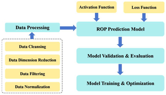
Figure 2.
Research flow chart of ROP prediction based on the BP neural network.
As shown in Figure 2, first, data processing is carried out, which includes data cleaning, feature dimensionality reduction, median filtering, and normalization. Then, the drilling prediction model is established, and the activation function and loss function are set. Subsequently, model training and optimization are conducted. Finally, model validation is carried out.
2.2. Dataset
A geological core drilling test bench based on a dual-motor drive is used to collect the main parameters during the drilling process [13], as shown in Figure 3. These parameters include the WOB, TOR, Q, RPM, and ROP. The experiment uses cubic concrete blocks measuring 150 mm × 150 mm × 150 mm, granite, and limestone to simulate the strata. Each different concrete block is used as a unit, with an 80/20 split for the training set and testing set. As shown in Figure 4, the concrete blocks are made from the same batch in order to reduce errors in the experiment. The sensor parameters are listed in Table 1, the sample parameters are listed in Table 2, and the properties of the geologic core drilling diamond-impregnated drill bits are shown in Table 3.
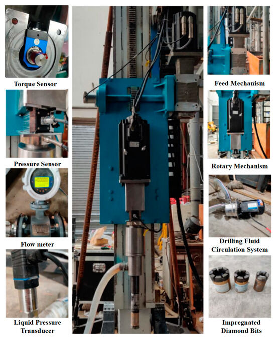
Figure 3.
Geological core drilling test rig based on a dual-motor drive.
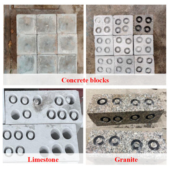
Figure 4.
Experiment sample.

Table 1.
Sensor parameters.
Table 2.
Sample parameters.
Table 3.
Design parameters of the diamond-impregnated bit in the experiments.
In order to investigate the relationship between drilling parameters such as drilling pressure, torque, slewing speed, mechanical drilling speed, pump volume, and depth of advance, the experimental rig adopts a constant-speed drilling model. The mechanical drilling speed is controlled at 1.39 m/h, 2.78 m/h and 4.17 m/h respectively. The rotary speed is 600 rpm, the pump volume is 600 L/min, and the drilling footage is 300 mm. This paper collected a total of 13,887 datasets through the geological core drilling test bench. Some of the data are shown in Table 4. Drilling data at the different ROPs are shown in Figure 5.
Table 4.
Drilling parameters.
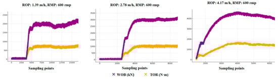
Figure 5.
Drilling data for the different ROPs.
From Figure 5, the trends of the TOR and WOB in the constant-speed drilling mode are similar, and the torque and drilling pressure slowly increase and eventually stabilize with the increase in feed. However, due to the different RPMs, the matching TOR and WOB drilling parameters are different for the same experimental samples drilled at the same drilling depth. At an ROP of 1.39 m/h and an RPM of 600 rpm, the TOR tends to stabilize at 600 N, and the WOB tends to stabilize at 2000 N·m. At an ROP of 2.78 m/h and an RPM of 600 rpm, the TOR tends to stabilize at 1000 N, and the WOB tends to stabilize at 3000 N·m. At an ROP of 4.17 m/h and an RPM of 600 rpm, the TOR tends to stabilize at 1500 N, and the WOB tends to stabilize at 4000 N·m. Therefore, it can be seen that by exploring the drilling parameters matching the lithology of each experimental stratum, we can find the complex relationships among them. Through the drilling parameters, it is possible to predict the characteristics of the stratum lithology in geological core drilling as well as to predict the real-time mechanical drilling speeds, thus achieving the purpose of optimizing the drilling speeds.
2.3. Data Preprocessing and Normalization
2.3.1. Data Correlation Analysis
Data correlation analysis can be used to determine the correlation between input and output variables, guiding further operations during modeling. This paper adopted the Pearson correlation coefficient method to analyze the correlation of variables such as weight on bit (WOB), torque (TOR), pump flow rate (Q), rotational speed (RPM), rate of penetration (ROP), bit wear, and bit cutting depth. Highly correlated parameters were selected as features. The calculation method is shown in Equation (5).
Here, represents the covariance equation of variables a and b; and indicate the standard deviation of variables a and b respectively; and represent the average of variables a and b; and n indicates the size of the dataset.
The results of the correlation analysis are shown in Figure 6. Due to the small number of experimental groups and minimal wear on the drill bit, the wear condition of the drill bit can be considered negligible; hence, the correlation between drill bit wear and the mechanical ROP is 0. Furthermore, because of the good drillability of the concrete blocks and the relatively shallow drilling depth, with each block drilled to a depth of 50 mm, the effect of the drill-bit cutting depth on the mechanical drilling rate is also minor, with a correlation of 0.08. Among these, the WOB, TOR, Q, and RPM have a high correlation with the mechanical ROP; therefore, these are used as feature values for modeling in this experiment.
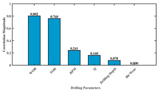
Figure 6.
Correlation analysis of drilling parameters.
2.3.2. Data Cleaning, Filtering, and Dimensionality Reduction
The original data include a lot of useless data, which will impact the precision accuracy. Data dimensionality reduction helps in obtaining the core structure of the data and enhances the accuracy of applications. In the data collected from the geological core drilling test bench, all the experiments used the same rotational speed. Due to the good drillability of the concrete blocks and the shallow drilling depth, it was observed and concluded that the influence of pump flow on the drilling speed in this experiment is extremely small and can be considered negligible. To improve the training accuracy of the model and reduce the computational complexity of the artificial neural network, the pump flow rate was removed from the drilling parameters as part of the dimensionality reduction process.
For the geological core drilling test rig, sensor measurement errors and initial calibration errors can cause a large amount of interfering noise, as well as frequent tripping of the drill string and situations such as sticking and balling during drilling. Additionally, secondary cutting of cuttings that are not promptly evacuated can lead to increased errors in drilling parameters and an increase in abnormal data points, thus requiring preprocessing of the drilling parameter data. A digital filter is an algorithm formed by a certain data logic that can filter out specific noise in the input signal. The weighted median filtering algorithm is a nonlinear signal processing technology based on order statistics theory that can effectively suppress noise. The filter window size can be set to L(L is odd), and the sample pixel in the filter window is {}. Then the output of a center-weighted median filter (CWMF) whose central weight is ( is an integer) is shown in Equation (6).
Here, indicates data replication, so = , , , (there are of ); median {} represents the median operation.
2.3.3. Normalization
Before using the BP neural network for network training and result prediction, it is necessary to normalize the data. Common normalization methods include linear function normalization (min–max scaling) and zero-mean normalization (z-score standardization). The purpose is to “stretch” the distribution of data across dimensions and to project them onto a similar scale range. Otherwise, due to the large range discrepancies in different types of collected data, problems such as slow convergence speed and long training time of the BP neural network may arise. This study uses linear normalization processing, as shown in Equation (7).
In the formula, and are the minimum and maximum values in the same column of data to be processed, and X is the current data being processed.
Due to the large range of the data, to improve data accuracy, the results after data preprocessing and normalization are taken to three significant figures. The data after preprocessing and normalization are shown in Table 5.
Table 5.
Drilling parameters after pretreatment and normalization.
3. Modeling Program
3.1. BP Neural Network Model Training
3.1.1. Loss Function
The loss function is primarily used during the model training phase. After each batch of training data is fed into the model, the forward propagation outputs the predicted values. The loss function assesses the distance between the predictions and the practical data. By employing back propagation, the model adjusts the parameters to narrow the loss, guiding the predictions to align with the practical data.
The mean squared error loss function is used to measure the distance between sample points and the regression curve. By minimizing the squared loss, the sample points can better fit the regression curve. The smaller the value of the mean squared error (MSE) loss function, the higher the precision of the sample data described by the prediction model. Therefore, to achieve the characteristic of regression for the results of this study, the mean squared error loss function was chosen for model training. The expression for the mean squared loss function (MSE) is shown in Equation (8).
3.1.2. Number of Hidden Layer Nodes
The hidden layer is an important component of the BP neural network, and the number of nodes in the hidden layer is a crucial parameter that determines the performance of the entire BP neural network. The node count in the BP neural network’s hidden layers greatly influences the prediction accuracy: too few nodes may lead to inadequate learning and necessitate more training cycles, impacting accuracy; too many nodes can extend the training time and raise the risk of overfitting. The hidden layer nodes in a BP neural network are shown in Equations (9) and (10).
Among these, z and n are the number of hidden and input layer nodes, m is the number of nodes in the output layer, and a is a constant between 0 and 10.
Since the BP neural network established in this paper has 3 input layer nodes and 1 output layer node, after multiple tests, the number of hidden layer nodes selected in this study is 5.
3.1.3. Learning Rate
The learning rate can control the pace at which the model learns. During training, it is common to set a dynamic learning rate based on the number of training epochs. Initially, a learning rate between 0.01 and 0.001 is advisable. After a certain number of epochs, it should gradually decrease, and by the time training is nearing completion, the decay of the learning rate should be more than 100 times.
3.1.4. Model Training
In machine learning, there is an unavoidable issue, which is the division of the test set and the training set. The purpose is to enhance the model’s generalization capability, prevent overfitting, and find the optimal tuning parameters. The training set is used for training the model, while the testing set is the dataset used to evaluate the trained model. This article uses the holdout method to divide the dataset, which involves directly splitting the original dataset into two mutually exclusive datasets, namely the training set and the testing set. Through continuous comparison and verification, this study ultimately randomly selected 80% of the data from the total dataset for the training set and 20% for the testing set. Using a sigmoid activation function, the characteristics of the forward propagation of information and the backward propagation of errors in the BP neural network were utilized to continuously adjust the weights of each training dataset. Through repeated trials, the learning rate of the model was set to 0.01. After 1000 training iterations, the backward propagation error of the model was controlled at around , finally determining the weights of each training dataset and completing the entire training of the BP neural network model.
3.2. Evaluation Index
For the trained model, there need to be evaluation metrics to judge the results after model testing. In this study, the most commonly used root mean square error (RMSE) and R-squared (R2) values were selected as evaluation metrics. These evaluation metrics can intuitively reflect the quality of the model, thereby indicating the accuracy of the experimental predictions for the mechanical ROP and the degree of fit with the original data.
- (1)
- Mean square error (MSE)
The MSE is the mean of the squared differences between the practical and predicted values. Lower MSE values suggest a more accurate model fit. This is specifically shown in Equation (11).
- (2)
- Root mean square error (RSME)
The RMSE is the square root of the MSE. It is relatively sensitive to outliers in the data. The specific definition is shown in Equation (12).
Here, is the predicted data, is the real data, N indicates the number of data points.
- (3)
- Mean absolute error (MAE)
The MAE is the average of the absolute differences between the practical and predicted values. A lower MAE signifies a more precise model alignment. This is specifically shown in Equation (13).
- (4)
- R value (R2_SCORE)
The R value is also called the R2_SCORE, which translates as the fitting coefficient. For a given variable, there is a series of observed values and corresponding predicted values . This measures how well the predicted values fit the true values. The R value is defined in Equation (14). The prediction model explains the proportion of the variance of the variables.
Here, is the predicted value, is the true value, and is the average of the true values.
Test Result Analysis
Using the trained BP neural network model, predictions were made for the data in the test set. Comparing the results of mechanical ROP predictions for granite, limestone, and concrete blocks with other neural network algorithms, evaluations were conducted using MAE, MSE, RMSE, and R2, as shown in Figure 7.
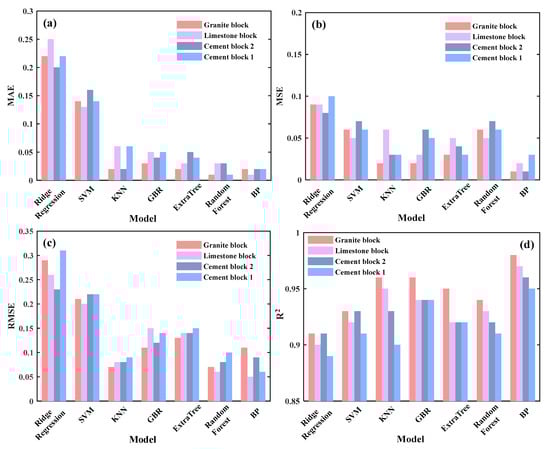
Figure 7.
Comparison of prediction results for the rate of penetration (ROP) using (a) MAE, (b) MSE, (c) RMSE, and (d) R2.
From Figure 7, it can be seen that both the regression algorithm and the BP neural network algorithm achieved good prediction results on different experimental samples, with prediction accuracies basically above 90%. Among them, the MAE and MSE are the smallest when compared with other algorithms, and the RMSE results are close to those of KNN and Random Forest, proving that the BP neural network has better prediction performance and smaller errors in drilling speed prediction.
3.3. Prediction of ROP in Mixed Formation
ROP is an important parameter for measuring the drilling efficiency, which is the depth of the drill bit into the rock per unit time. The level of ROP directly affects the progress and cost of the drilling operation. In practical core drilling, selecting suitable drilling parameters and optimizing the ROP can effectively improve the efficiency of drilling operations. To simulate a real complex-formation environment and to verify the prediction performance of the regression algorithm and the BP neural network in mixed formations, all the drilling experimental data were mixed and then randomly divided into training, validation, and testing sets at a ratio of 70%, 15%, and 15% respectively. After the model was trained, we evaluated the mechanical ROP prediction results, as shown in Figure 8.
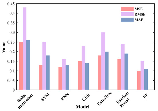
Figure 8.
Comparison of prediction results for the mixed-formation experimental sample data.
From Figure 8, it can be seen that the evaluation metrics of the BP neural network show better prediction performance compared with the other algorithms. Using R2 as the evaluation metric, the prediction results of each algorithm are shown in Figure 9.
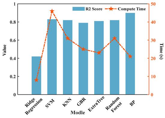
Figure 9.
Comparison of the predicted R2 and the operation time.
From Figure 9, it can be seen that after mixing the data, the difficulty of predicting the mechanical ROP increases. Compared with the previous prediction results, the MSE, RMSE, MAE, and other metrics have increased, the R2 value has decreased, and the required computation time has significantly increased. The average prediction accuracy is around 80%. Among these, the ridge regression algorithm requires the least computation time, but due to its poor prediction accuracy, it was excluded. In contrast, the BP neural network algorithm’s MSE, RMSE, MAE, and R2 metrics are better than those of other algorithms, with a prediction accuracy of 90%. At the same time, the computation time needed is only about 20 s, which can meet actual needs. The predicted mechanical ROP values were compared with the actual mechanical ROP values, and the comparison results are shown in Figure 10.
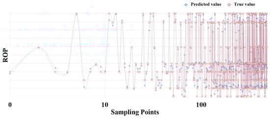
Figure 10.
Comparison between the real value and the predicted value of the ROP.
The blue line in the figure represents the predicted values, and the red line represents the true values. As can be seen from the figure, the error between the actual values and the predicted values is small. Through comparison and calculation, the root mean square error of the model’s prediction results is 0.059, indicating that the prediction accuracy of the model can reach 94.1%. The R2 value calculation result is 0.966, meaning the fit of the predicted mechanical ROP values to the true values can reach 96.6%. This indicates that the neural network performs well in predicting this formation and can effectively predict drilling speed optimization.
4. Conclusions
In the field of geological core drilling, due to the complex geomechanical environment characterized by “three highs and one disturbance” during deep geological drilling, issues such as non-linearity, strong coupling, and strong interference are prominent. These pose challenges for drilling speed prediction and optimization, as well as for the development of automated drilling machines. Utilizing the BP neural network algorithm can better uncover the relationships between drilling parameters. This study analyzed the drilling parameters collected from the geological core drilling test bench. Through the different ROP data collected for the same rock, it was found that there is a complex relationship between drilling parameters such as the ROP, WOB, and TOR, and we verified that predicting the real-time ROP by drilling parameters is possible. Subsequently, we constructed a BP neural network model and used the established model to predict the mechanical ROP. Additionally, by comparing the prediction structures with other neural networks, the results showed that the BP neural network has significant advantages in drilling speed prediction. By analyzing the prediction results of the mechanical ROP, the final test results showed an error of less than 5.9%, indicating that the trained model can achieve a prediction accuracy of 94.1% for the mechanical ROP. The study also found that the fit between predicted values and actual values could reach 96.6%, demonstrating that using the BP neural network to predict the mechanical ROP in geological core drilling is feasible. This also provides validation that the established neural network model has high accuracy and good generalization ability. However, this study only validated the feasibility of drilling speed prediction under single-formation conditions and did not utilize the prediction results for further optimization of the mechanical ROP in geological core drilling. Therefore, the proposed model still requires further research and refinement.
Author Contributions
Conceptualization, Z.Z.; Methodology, D.G. and M.J.; Validation, D.G.; Investigation, Y.Z.; Resources, Z.Z. and Y.H.; Writing—original draft, M.J.; Writing—review & editing, D.G., Y.Z. and J.L.; Visualization, Y.Z.; Supervision, Z.Z.; Funding acquisition, Y.H. All authors have read and agreed to the published version of the manuscript.
Funding
This work was supported by National Key R&D Program of China (2016YFE0202200).
Institutional Review Board Statement
Not applicable.
Informed Consent Statement
Not applicable.
Data Availability Statement
The original dataset of the experiment can be found from (https://dx.doi.org/10.21227/vqkd-7f86, accessed on 1 August 2022).
Conflicts of Interest
The authors declare no conflict of interest.
References
- Caicedo, H.U.; Calhoun, W.M.; Ewy, R.T. Unique ROP predictor using bit-specific coefficient of sliding friction and mechanical efficiency as a function of confined compressive strength impacts drilling performance. In Proceedings of the SPE/IADC Drilling Conference and Exhibition, Amsterdam, The Netherlands, 23–25 February 2005. [Google Scholar]
- Barbosa, L.F.F.M.; Nascimento, A.; Mathias, M.H.; de Carvalho, J.A., Jr. Machine learning methods applied to drilling rate of penetration prediction and optimization—A review. J. Pet. Sci. Eng. 2019, 183, 106332. [Google Scholar] [CrossRef]
- Shokry, A.; Elkatatny, S.; Abdulraheem, A. Real-time rate of penetration prediction for motorized bottom hole assembly using machine learning methods. Sci. Rep. 2023, 13, 14496. [Google Scholar] [CrossRef] [PubMed]
- Youssef, A.S.; Elkatatny, S.; Abdulraheem, A.; Rahmatullah, I. Real-Time Rate of Penetration Prediction for Motorized Bottom Hole Assembly Using Artificial Intelligence. In Proceedings of the ARMA US Rock Mechanics/Geomechanics Symposium, Golden, CO, USA, 23–26 June 2024. [Google Scholar]
- Rommetveit, R.; Bjørkevoll, K.S.; Halsey, G.W.; Larsen, H.F.; Merlo, A.; Nossaman, L.N.; Sweep, M.N.; Silseth, K.M.; Ødegaard, S.I. Drilltronics: An Integrated System for Real-Time Optimization of the Drilling Process. In Proceedings of the SPE/IADC Drilling Conference and Exhibition, Dallas, TX, USA, 2–4 March 2004; Available online: https://onepetro.org/SPEDC/proceedings/04DC/All-04DC/SPE-87124-MS/72307 (accessed on 24 November 2022). [CrossRef]
- Iversen, F.P.; Cayeux, E.; Dvergsnes, E.W.; Gravdal, J.E.; Vefring, E.H.; Mykletun, B.; Torsvoll, A.; Omdal, S.; Merlo, A. Monitoring and Control of Drilling Utilizing Continuously Updated Process Models. In Proceedings of the 2006 IADC/SPE Drilling Conference, Miami, FL, USA, 21–23 February 2006. [Google Scholar]
- Gan, C.; Cao, W.; Wu, M.; Chen, X.; Hu, Y.; Wen, G.; Gao, H.; Ning, F.; Ding, H. An online modeling method for formation drillability based on OS-Nadaboost-ELM algorithm in deep drilling process. IFAC-PapersOnLine 2017, 50, 12886–12891. [Google Scholar] [CrossRef]
- Hegde, C.; Soares, C.; Gray, K.E. Rate of Penetration (ROP) Modeling Using Hybrid Models: Deterministic and Machine Learning. In Proceedings of the 6th Unconventional Resources Technology Conference, Houston, TX, USA, 23–25 July 2018. [Google Scholar]
- Ding, S.; Su, C.; Yu, J. An optimizing BP neural network algorithm based on genetic algorithm. Artif. Intell. Rev. 2011, 36, 153–162. [Google Scholar] [CrossRef]
- Hazbeh, O.; Aghdam, S.K.; Ghorbani, H.; Mohamadian, N.; Alvar, M.A.; Moghadasi, J. Comparison of accuracy and computational performance between the machine learning algorithms for rate of penetration in directional drilling well. Pet. Res. 2021, 6, 271–282. [Google Scholar] [CrossRef]
- Lawal, A.I.; Kwon, S.; Onifade, M. Prediction of rock penetration rate using a novel antlion optimized ANN and statistical modelling. J. Afr. Earth Sci. 2021, 182, 104287. [Google Scholar] [CrossRef]
- Su, K.; Da, W.; Li, M.; Li, H.; Wei, J. Research on a drilling rate of penetration prediction model based on the improved chaos whale optimization and back propagation algorithm. Geoenergy Sci. Eng. 2024, 240, 213017. [Google Scholar] [CrossRef]
- Zhou, Z.; Hu, Y.; Liu, B.; Dai, K.; Zhang, Y. Development of Automatic Electric Drive Drilling System for Core Drilling. Appl. Sci. 2023, 13, 1059. [Google Scholar] [CrossRef]
- Mohamadian, N.; Ghorbani, H.; Wood, D.A.; Mehrad, M.; Davoodi, S.; Rashidi, S.; Soleimanian, A.; Shahvand, A.K. A geomechanical approach to casing collapse prediction in oil and gas wells aided by machine learning. J. Pet. Sci. Eng. 2021, 196, 107811. [Google Scholar] [CrossRef]
Disclaimer/Publisher’s Note: The statements, opinions and data contained in all publications are solely those of the individual author(s) and contributor(s) and not of MDPI and/or the editor(s). MDPI and/or the editor(s) disclaim responsibility for any injury to people or property resulting from any ideas, methods, instructions or products referred to in the content. |
© 2024 by the authors. Licensee MDPI, Basel, Switzerland. This article is an open access article distributed under the terms and conditions of the Creative Commons Attribution (CC BY) license (https://creativecommons.org/licenses/by/4.0/).