Article

Path Planning Optimization of the Load Transport Process Using Heuristic Algorithms

1
Department of Mechanics and Machine Design Fundamentals, Faculty of Mechanical Engineering, Czestochowa University of Technology, Dąbrowskiego 73, 42-201 Częstochowa, Poland
2
Department of Advanced Computational Methods, Faculty of Science and Technology, Jan Dlugosz University in Czestochowa, Armii Krajowej 13/15, 42-200 Częstochowa, Poland
3
Department of Applied Mechanics, Faculty of Mechanical Engineering, VŠB-Technical University of Ostrava, 17. listopadu 15/2127, 708 33 Ostrava, Czech Republic
*
Author to whom correspondence should be addressed.
Appl. Sci. 2024, 14(21), 9940; https://doi.org/10.3390/app14219940
Submission received: 30 September 2024 / Revised: 23 October 2024 / Accepted: 28 October 2024 / Published: 30 October 2024
(This article belongs to the Section Mechanical Engineering)

Abstract

:
The paper presents the process of optimizing the duty cycle of a rotary crane. The minimization of the carried load’s trajectory was chosen as the objective function. The research was conducted using the genetic algorithm and the particle swarm algorithm. The influence of particular algorithm parameters on the obtained optimal solution was characterized. For the obtained best case, the inverse kinematics problem was solved, allowing us to determine the control functions of individual crane members. The presented redundant system was solved with the use of an algorithm for temporarily limiting the movement of specific kinematic pairs. On the basis of the obtained results, it was determined which of the algorithms used is more favorable, taking into account the crane’s operational safety and lifting capacity.

1. Introduction

The load transport process in an industrial hall or on a construction site is one of the basic and key operations without which efficient work would be impossible. The primary motivation for optimizing these processes lies in the need to enhance efficiency, safety, and precision in cargo transport, especially in industries such as construction, manufacturing, and logistics, where the cargo can range from heavy construction materials to delicate electronic components. The calculated optimization models can directly benefit operations involving heavy cranes, gantries, and automated guided vehicles (AGVs). The main goal of research on this issue is to improve efficiency, safety, and comfort at work. The increase in computational capabilities makes it possible to optimize the duty cycle of transport machines, not only in the case of repetitive activities but also in the case of single transfers. The continuous development of information technology and the growing interest in cyber-physical systems determine the increasingly common work without human intervention or with only supervisory oversight. Determination of the optimal path in this case can be sent directly to the control system, which can reduce manual control of the machine.
In the literature on crane optimization studies, two main divisions can be distinguished: crane construction or its duty cycle. The minimization of impacts caused by the Coriolis force at the stage of selecting the system parameters and crane structure is presented in reference [1]. The optimization was confirmed by dynamic analysis, which allowed for a significant reduction in the value of dynamic overloads already at the design stage, resulting in a cheaper and lighter structure. Based on the mathematical model, optimization criteria were formulated for each crane mechanism. In addition to minimizing Coriolis force impacts, the focus was also on reducing load fluctuations. Reference [2] presents the optimization of the construction design of work platforms. A 3D model was developed in the SolidWorks environment, and then a dynamic analysis was carried out to determine the construction parameters of the lift. The results of the analysis were compared with the mathematical model and validated. A simulation model that allows determining the interaction between mobile cranes and the accompanying work crews is presented in reference [3]. Optimal crane and crew configurations have been determined to minimize construction costs and unloading time. Optimization was carried out based on a multi-functional genetic algorithm. The authors of [4] present a method to optimize the configuration of a gantry crane using a two-phase model. Minimization of costs during reloading operations was adopted as the objective criterion, taking into account all the limitations resulting from the nature of the crane’s operation. Based on experimental verification, it was found that the proposed method can effectively reduce operating costs while maintaining the implementation time. The application of the genetic algorithm during the load positioning stage is presented in reference [5]. The optimization was based on the method of selecting the driving function of the crane platform rotation. As a result of the applied method, the desired final position of the load and the minimization of the crane’s duty cycle time were obtained. Reference [6] presents the issue of synchronizing the work of a quay crane and a shipyard truck. The objective function was to minimize the total time needed to complete the unloading and transport operations of all containers. Optimal solutions were obtained using the adaptive particle swarm algorithm (APSO), in which all parameters were selected automatically. The issue of precise operation of mobile cranes, taking into account the complexity and dynamics of construction sites, is shown in reference [7], where an approach to determining the location of cranes based on simulation studies is presented. The method of data processing and the BIM (Building Information Modeling) concept were used to optimize the location of the cranes, and the boundary contour method was used to detect collisions and ensure work safety. Optimization of the storage area on construction sites where a tower crane is located is presented in [8]. The presented mathematical model was used to calculate the optimal positions due to the cost minimization criterion. The optimal positions of the cranes on the construction site were calculated while the algorithm was running, which allowed for the free movement of obstacles in the analyzed working area. Reference [9] presents a method for optimizing the trajectory of rotating cranes based on the integration of the A* algorithm with a time-optimal approach, which allows smooth obstacle avoidance and minimizes the movement time. The A* algorithm is modified to better control the rotation angles and the movement of the crane rope, taking into account different priorities for individual movement elements, in accordance with the dynamics and constraints. The trajectory is expressed by a polynomial function, which provides effective load tilt damping, as shown by the simulation results. The A* algorithm was also used in [10] to develop an improved hybrid version with multi-body constraints that addresses the problems of traditional path planning methods for non-holonomic mobile robots, such as approaching too close to obstacles, unnecessary backtracking, and excessive turns. By dynamically weighting the heuristic function and optimizing the path costs, the algorithm increases the minimum obstacle distance by more than 50%, reduces the number of unnecessary backtracking and turning, and shortens the total navigation time by 14.2% on average, thus improving the robot navigation performance. In [11], the metaheuristic optimization algorithm Grey Wolf Optimizer (GWO) was applied in the process of designing offshore cranes. GWO allowed for automatic configuration of design parameters, which increased the maximum safe lifting capacity of the crane and reduced its weight, and its effectiveness was confirmed in comparison with other evolutionary algorithms. In turn, in [12], a new algorithm Puma Optimizer (PO) was presented, inspired by puma intelligence, which, thanks to the hyper-heuristic mechanism, automatically adjusts the exploration and exploitation phases to the characteristics of the problem. PO proved to be more effective than other optimization algorithms, obtaining better results in 27 out of 33 benchmarks and in tasks such as community detection and feature selection. In [13], a heuristic algorithm for optimizing the container retrieval process was proposed, which minimizes the number of their movements and shortens the crane operation time. The algorithm’s effectiveness was confirmed based on tests conducted on 70 problems, and its computational efficiency allows for quick decision-making in practical applications. The problem of planning lifting routes for all-terrain cranes in complex environments was presented in [14], where energy and time costs and operational risk were optimized. For this purpose, a parallel genetic algorithm was used, which generates safe lifting routes, meeting the requirements for collision avoidance and operational constraints. The authors of [15] presented an algorithm based on simulated annealing (SA) for optimizing the retrieval phase in automatic warehouses for metal bundles. This algorithm improves operational efficiency by minimizing the differences between the ordered and retrieved material in terms of quality and weight, which increases the number of missions performed per hour.
While significant efforts have been made in the field of crane optimization, much of the research does not translate directly into broader applications. This paper aims to fill this gap by presenting potential areas where optimization models can be applied, such as load-handling automation in complex industrial environments. Trajectory optimization is one of the most frequent topics in the study of load transport. Among the optimization methods used in these issues, heuristic methods are most often used, which include classical evolutionary algorithms or their modifications. The issues of trajectory optimization with the use of evolutionary algorithms have been described in detail in [16]. The authors, using the cuckoo search algorithm (CS), optimized the 3D trajectory of a body submerged in water. They compared their results with the two most popular algorithms: genetic algorithm and particle swarm optimization. The authors of the paper noticed that the CS algorithm is a more advantageous solution in the case of determining the trajectory of the body based on the minimum terminal error and maximum terminal velocity. In [17], GA and PSO were used to optimize the coverage of a large area by unmanned aerial vehicles. The authors solve the traveling salesman problem, a mathematical model that has been developed that allows for planning and optimizing the path of vehicles. The advantages of both algorithms were used to develop a method that allows for trouble-free exit from the local minimum while maintaining a better quality of solutions in computational time. The subject of trajectory optimization in various industries has been extensively described among others in review papers [18,19,20].
Heuristic algorithms, especially their hybrid combinations, are widely used not only in cargo transportation but also in other industries such as humanitarian logistics, e-commerce delivery, and distribution network management. These studies illustrate their effectiveness in solving complex optimization problems in different contexts. Reference [21] proposes a multi-objective model for the location and routing problem (LRP) in emergency logistics, which takes into account the urgency of delivering relief materials after disasters such as earthquakes or COVID-19. To solve this NP-hard problem, a hybrid metaheuristic algorithm combining Discrete Particle Swarm Optimization (DPSO) and Harris Hawks Optimization (HHO) is used, with additional improvement strategies, which allowed for improving the accuracy of the results and more effectively avoiding local minima. The optimization of takeaway food delivery, where a model combining drones and couriers in a common delivery network with multiple distribution centers, was developed in [22]. Using a two-stage algorithm based on clustering and an improved tabu algorithm, delivery routes were optimized, which contributed to reducing costs, reducing the number of couriers needed, and increasing customer satisfaction. Reference [23] focused on the optimization of the “last mile” in e-grocery using autonomous delivery vehicles (ADVs). A model of a two-tier distribution network with a mixed fleet of vehicles was developed, where traditional delivery vehicles serve the first tier and autonomous vehicles serve the second tier. The problem was solved using a hybrid GA-PSO algorithm, and the results showed significant reductions in transportation costs and emissions. In [24], the authors discussed the logistics of perishable products under uncertain demand conditions. A multi-period optimization model was used, including both forward and reverse logistics, with three main objectives: minimizing costs, environmental impact, and ensuring just-in-time delivery. The problem was solved using a hybrid GA-PSO algorithm supported by the CPLEX solver, and the study on the example of an enterprise in Shanghai confirmed the effectiveness of the proposed strategies.
This work concerns the problem of optimizing the trajectory of the transported load using a rotary crane. This paper seeks to determine whether the Genetic Algorithm (GA) or Particle Swarm Optimization (PSO) is superior in terms of optimizing the crane’s trajectory. A detailed comparison is made in terms of computation time, solution quality, and algorithmic convergence. Such distinctions are necessary for understanding the strengths and weaknesses of each algorithm in practical scenarios. Furthermore, specific choices regarding algorithm parameters, such as mutation probability and population size, were justified based on preliminary test results [25,26], ensuring their applicability to various scenarios. In addition, various parameters of these algorithms are analyzed. The inverse kinematics solution presented in this paper allows us to determine the characteristic variables of the crane and to determine which of the proposed algorithms will prove to be more advantageous in terms of work safety. Moreover, although this study focuses on a single-objective approach, it is important to recognize that this choice limits the scope of the optimization process.
For the purposes of this work, the following research hypothesis was defined: The choice of the PSO (Particle Swarm Optimization) algorithm in the optimization process is more beneficial due to the higher computational speed compared to the genetic algorithm (GA), while maintaining a comparable quality of solutions, which results in small differences in the final outcomes between PSO and GA.
The present study is composed of six main sections. Section 1 concerns the introduction, where an overview of the available solutions to the analyzed subject and the motivation for undertaking the research are presented. Section 2 presents a short description of the problem, in which the working environment, optimization criterion and selected simulation parameters are presented. Section 3 shows a solution to the optimization problem divided into the two most commonly used heuristic algorithms: genetic algorithm and particle swarm optimization. Section 4 concerns the solution of the inverse kinematics of the machine in order to map the movement of the load along the determined optimal trajectory. Section 5 presents a discussion of the results, and Section 6 concludes the paper.

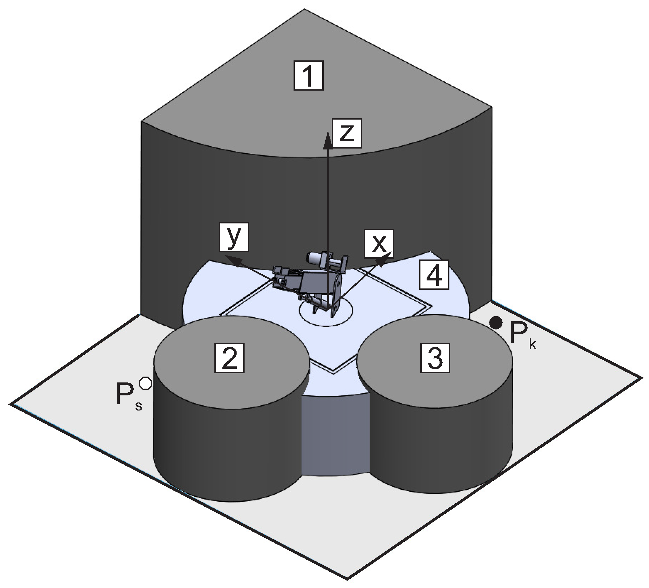
2. Description of the Problem

The working environment (Figure 1) has additional constraints (1, 4) and obstacles (2, 3). The limitations result from the range of working movements that can be performed by the crane ([27]), while the obstacles can be interpreted as buildings or other machines located in its work zone. Forbidden areas are defined as geometric shapes (cylinders) that can be described by their height (h) and diameter (d). The proposed work environment model can be applied to industrial settings where precise crane movements are essential to navigating complex arrangements of obstacles and other equipment. These conditions include, but are not limited to, construction sites and warehouses where the safe transfer of heavy loads is critical to operational efficiency. The key assumption of this problem is to transfer the load from the starting point P s to the endpoint P k by the shortest possible path while maintaining work safety and determining the characteristic variables that allow the crane to map the optimal trajectory.
Based on the assumptions made, the single-criteria optimization objective function will have the form [25,26]:
f 1 = L ( 1 + K 1 ) m i n ,
where L—trajectory length and K 1 —penalty function.
In three-dimensional problems, the penalty function can be defined as [26]:
K 1 = λ j n i m k j i
The individual components of Formula (2) take the form:
A j i = 1 for d j i < r j 0 for d j i r j
B j i = 1 for z H j + h j & z h j 0 for z > H j + h j & z < h j 0 for z < H j + h j & z < h j 0 for z > H j + h j & z > h j
k j i = A j i B j i 1 d j i r j
where z i is the designated trajectory point on the Z-axis, H j is the height of the obstacle, h j is the distance between the obstacle and ground, d i j is the distance between the trajectory point and the obstacle center, r j is the radius of the obstacle, j is the number of obstacles, i is the number of trajectory points, k is the trajectory number of an iteration, λ is the scale coefficient, n is the sum of obstacles and m is the sum of trajectory points.
The penalty function, which has been presented in the objective function, takes into account, among others, the following cases: one of the crane’s points is in an obstacle or there is a collision between the crane’s members. If one of these conditions is met, the objective function increases its value by the penalty function. The subject of appropriate selection of the penalty function has been extensively described in the papers [28,29].
The optimization process was carried out using two heuristic algorithms: the classic genetic algorithm (GA) and the particle swarm optimization algorithm (PSO). The choice of parameters for both algorithms, such as population size and mutation rates for GA or swarm size for PSO, was made based on preliminary tests, to ensure optimal performance for the crane operating environment. These choices were critical to minimize the impact of local minima on solution quality and convergence time [25,26]. All tests were performed on a Fujitsu Esprimo C720 computer (Fujitsu Technology Solutions, Augsburg, Germany) with the following parameters: CPU Intel(R) Core(TM) i5-4590 @3.30 GHz, RAM 8 GB, Intel(R) HD Graphics 460. Both heuristic algorithms have been implemented in Matlab R2022b software through self-written scripts and functions.
The parameters of the working space adopted for the research are as follows:
  • Co-ordinates (in mm) of the starting point P s ( 600 , 800 , 1 ) ,
  • Co-ordinates (in mm) for the endpoint P k ( 1100 , 300 , 1 ) ,
  • The height of the obstacles: h 1 = 1360 mm, h 2 = 650 mm, h 3 = 600 mm, h 4 = 560 mm,
  • The diameter of the obstacles: d 1 = 1500 mm, d 2 = 4400 mm, d 3 = 440 mm, d 4 = 810 mm,
  • Working area (in mm): x [ 1255 , 1255 ] ,   y [ 1255 , 1255 ] ,   z [ 0 , 1360 ] .
In order to represent the trajectory of a load with smooth transitions, a B-spline curve was selected, which is characterized by introducing additional auxiliary points in addition to the start and endpoints. The smooth trajectory allows for uninterrupted transport of the load, which ultimately reduces the phenomenon of rope swinging. Auxiliary points are selected randomly, and during the optimization process, they can move according to the determined trajectory. However, they determine the final shape of the curve.

3. Heuristic Algorithms

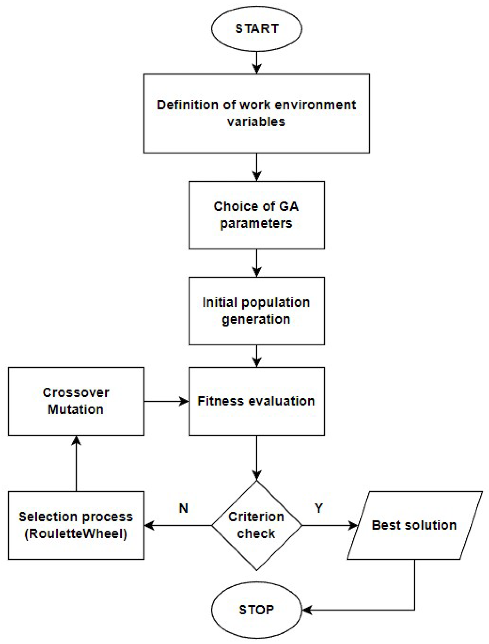
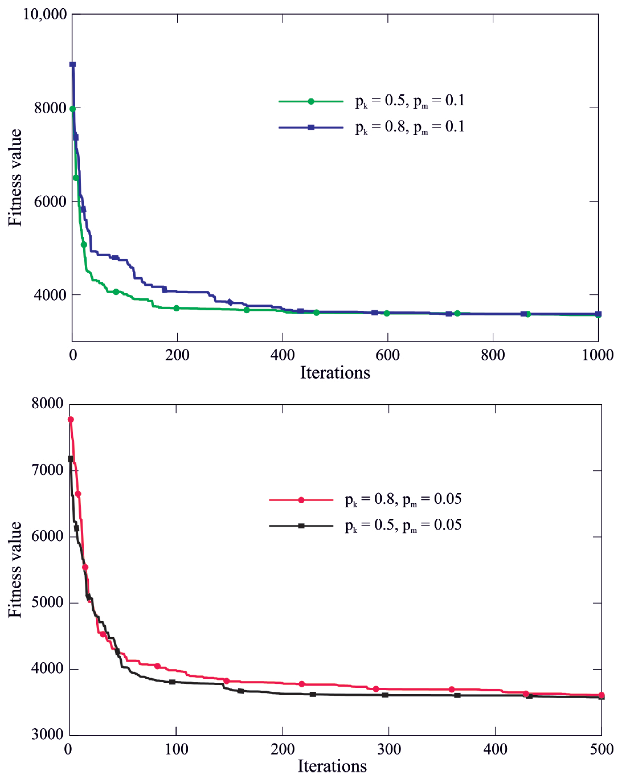
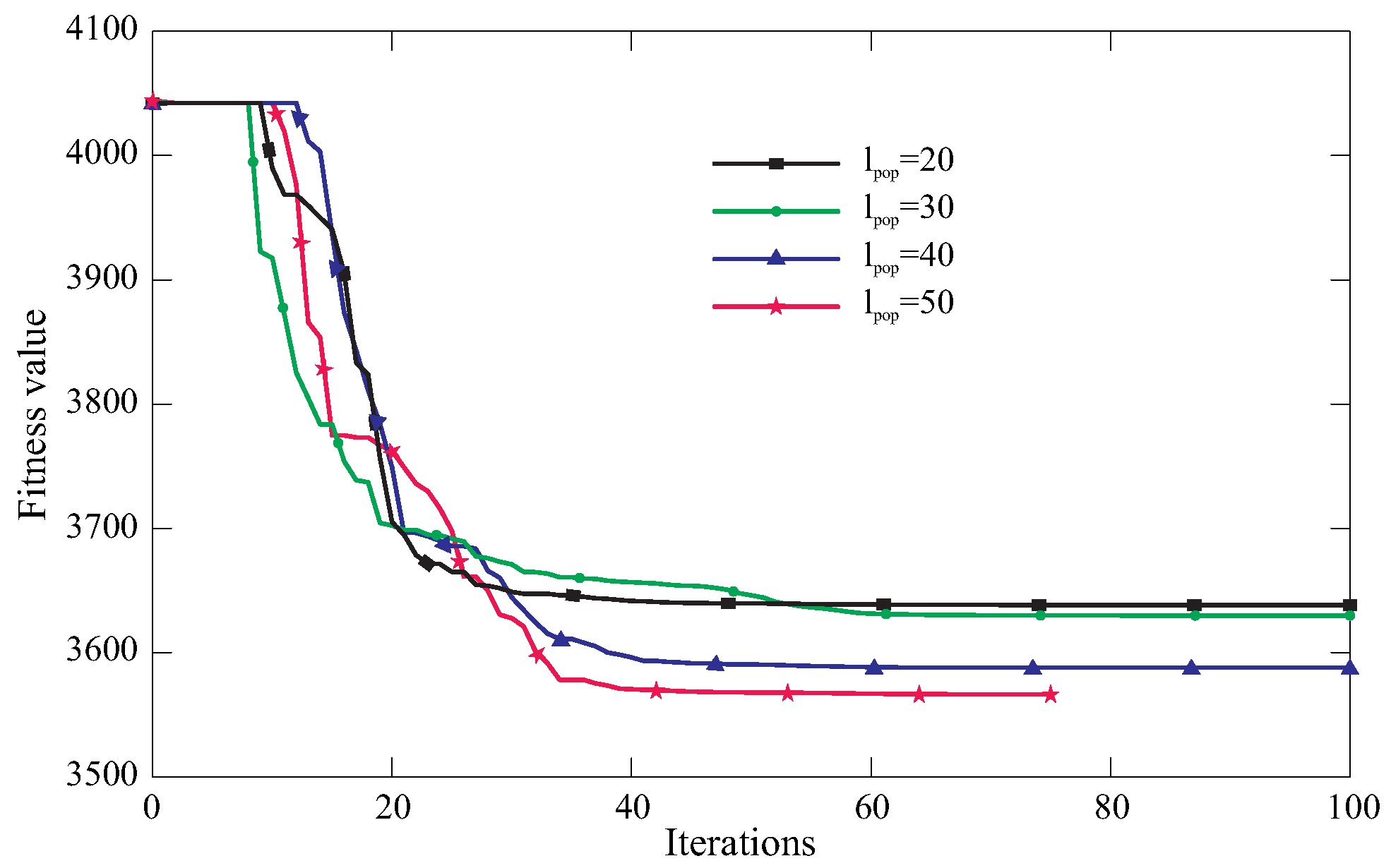
3.1. Genetic Algorithm

The principle of operation of the classical genetic algorithm, which was used in this work, can be presented in the following points [25,30]:
  • Generate (randomly) a starting population of n-chromosomes, which are the initial solution to the problem,
  • Calculate the objective function (adaptation assessment), which allows for determining the quality measure of individuals,
  • Terminate the genetic algorithm when the ending criterion of the algorithm is met,
  • If the criterion is not met, a new population of individuals is created by applying the selection process and genetic operators, which is again subjected to the stage of the fitness assessment.
The optimization process using the genetic algorithm is shown in Figure 2. The criterion check for the GA algorithm is based on the maximum number of generations. The algorithm stops working when it reaches a predetermined number of generations. The following operators were selected and implemented: the roulette method in the selection process, one-point crossover, and bit string mutation. The course of the fitness function for the best results from the analyzed variants is shown in Figure 3.
For each of the analyzed variants, calculations were performed 10 times, with the following characteristic parameters of the algorithm changed: crossing probability ( p k = 0.5 , p k = 0.8 ), mutation probability ( p m = 0.05 , p m = 0.1 ), number of waypoints ( i = 8 , 10 , 12 ) , number of populations ( l p o p = 50 , l p o p = 100 ) and number of iterations ( i t = 500 , 1000). The number of computations was chosen based on previous initial tests that analyzed differences in results. The calculations were repeated 10 times to balance the computational effort with the statistical robustness of the results, which is standard practice in similar optimization studies. In the initial tests, it was observed that with the number of repetitions exceeding 10, the changes in the results were insignificant. The results of the shortest trajectories are presented in Table 1, Table 2, Table 3 and Table 4, with the best solution presented for each analyzed case.
In the case of the genetic algorithm, the optimal (shortest) trajectory was obtained for the case p k = 0.5 , p m = 0.1 , l p o p = 100 , i = 8 , i t = 1000 , which was 3564 mm. Analyzing the obtained simulation results (Table 1, Table 2, Table 3 and Table 4), it was noticed that the genetic algorithm determines the shortest trajectory for a different number of intermediate points and for a larger number of populations ( l p o p = 100 ). It can also be concluded that the number of iterations does not significantly improve the performance of the algorithm. The shortest trajectories were obtained for different probability values both for the number of iterations i t = 500 and i t = 1000 . It was also found that for the analyzed work cycle, the number of intermediate points during the calculations should not exceed 10—for cases in which 12 intermediate points were taken into account, the worst results were obtained. A detailed analysis of population size ( l p o p ) showed that larger populations produced more consistent results. Smaller populations produced more variability, indicating that tuning population size may be a key factor in improving algorithm performance. The most important parameters of the genetic algorithm, such as the probability of crossing and mutation, have a large impact on the optimal solution obtained. Better results were obtained for a higher value of mutation probability ( p m = 0.1 ), while an increase in crossover probability results in worse results.

3.2. Particle Swarm Optimization

The particle swarm algorithm, which is inspired by swarm intelligence, was proposed by James Kennedy and Russel Eberhart in 1995 [31]. Since its development, the PSO algorithm has been improved many times, e.g., by transforming the equations of particle motion, resulting in a combination of the global and local versions [25].
The principle of operation of the PSO algorithm can be presented in the following steps [32,33]:
  • Specifying the input data,
  • Random selection of particle velocities and positions,
  • Calculation of the objective function,
  • Determination of the best local ( p m ) and global ( g m ) position of the particle,
  • Speed and location update,
  • Recalculation of the objective function,
  • Verification and update of location parameters ( p m and g m ),
  • Assignment of the optimal solution.
The appropriate choice of coefficients ( κ , w and c 1 ,   c 2 ) has a large impact on the acceleration of particle motion during numerical simulations. The selection of the PSO algorithm parameters was the subject of many works [26,34,35,36,37], in which appropriate values were determined to obtain the desired results. Based on the aforementioned works, the parameters of the particle swarm algorithm can be characterized as follows:
  • The squeeze factor ( κ ) prevents a sudden increase in speed and makes it easier to obtain population convergence,
  • Learning coefficients ( c 1 ,   c 2 ) determine the range of motion of the particle during iteration,
  • The weighting factor (w) maintains a balance when looking for a local and global solution.
During the simulation, the following values characteristic of the PSO algorithm were adopted: κ = 0.7 , w = 1 , λ = 0.5 , c 1 = 1.49445 and c 2 = 1.49445 . The scheme of PSO algorithm is presented in Figure 4. The criterion check for the PSO algorithm is based on the maximum number of iterations. The algorithm stops when a fixed number of iterations is reached. The course of the fitness function for the best results from the analyzed variants is shown in Figure 5.
Numerical simulations were carried out for the proposed objective function Equation (1) and with various parameters of the PSO algorithm. The choice of these parameters, in particular the learning coefficients and the weighting factor, had a significant impact on both the speed of convergence and the quality of the solutions. The balance between local and global exploration ensured that the algorithm avoided local optima. The operation of the algorithm (calculation time) and the obtained results depend on the selection of parameters [34,38]. The most important parameters include the learning coefficient, the number of populations (swarm), the number of auxiliary points (in the indirect method analyzed in this paper) and the number of iterations.
In this paper, for each of the analyzed cases, simulations were carried out ten times, with the following algorithm parameters changed: number of auxiliary points ( i = 2 , 3 , 4 , 5 ) , number of population ( l p o p = 20 , l p o p = 30, l p o p = 40, l p o p = 50) and the number of iterations ( i t = 25 , 50 , 75 , 100 ). In total, 256 numerical simulations were carried out, the results of which are presented in Table 5, Table 6, Table 7 and Table 8 and in Figure 6, Figure 7, Figure 8, Figure 9, Figure 10 and Figure 11 in the form of projections of the optimal trajectory for a different number of populations. The results show the average value for the individual results.
The shortest trajectory of all analyzed variants, 3566 mm, was obtained for the case l p o p = 50 , i = 5 , i t = 75 . Further analysis of the results suggests that increasing the number of iterations generally improves the quality of the solution, especially for larger populations, but this effect diminishes after 75 iterations. This highlights the potential benefit of dynamically adjusting the number of iterations based on early convergence results. Taking into account the obtained numerical results (Table 5, Table 6, Table 7 and Table 8), it can be concluded that the PSO algorithm finds the shortest trajectory for the maximum number of auxiliary points ( i = 5 ), but at a different number of iterations ( i t = 75 or i t = 100 ). For a population of l p o p = 20 , the shortest trajectory is 3638 mm. The difference in this case from the optimal trajectory is 2%, while the time needed to perform the calculations was shorter by 0.5 s. For the calculations shown in Table 6 ( l p o p = 30 ), the shortest trajectory is 3629 mm, and the difference from the optimal trajectory is 1.8%. The calculation time in this case was 1.91 s shorter. In the case when the population number is 40, the length of the trajectory is 3587 mm. However, the time needed to complete the calculations was longer than in the case of the optimal trajectory and amounted to 29.2 s. The difference in length did not exceed 1%.
It was also observed that increasing the number of population leads to a shorter trajectory (Figure 6, Figure 7 and Figure 8). The projection of the trajectory onto the XY axis (Figure 6) is similar for each of the analyzed population numbers. This similarity is due to the fact that the search space is simpler and less complex, which makes it easier for particles to converge to similar solutions. Particles show less tendency to scatter in this space, which leads to more similar results. In the XY plane, particles can move in a more regular and predictable environment, which is influenced by certain constraints of the crane operation and the presence of obstacles, which additionally stabilizes the optimization results in this plane. However, the differences appear in the projection of the trajectory on the XZ and YZ axes (Figure 7 and Figure 8). Better solutions are obtained for a larger number of auxiliary points ( i = 3 and i = 5 ), which is caused by the method of describing the trajectory using a B-spline curve. Taking into account additional points between obstacles makes it more “flexible”—the algorithm can better adjust the curve to the desired trajectory. Analysis of the impact of auxiliary points shows that selecting more auxiliary points increases the flexibility of the algorithm in navigating the complex obstacle environment, but above a certain point, the improvement becomes insignificant. The influence of the number of auxiliary points is shown in Figure 9, Figure 10 and Figure 11. For the number of auxiliary points i = 3 and i = 5 , a very similar course of the trajectory can be seen (Figure 9), in contrast to the other points ( i = 2 and i = 4 ). In Figure 10 and Figure 11, the differences between i = 3 and i = 5 are greater, but similar trends can also be observed.

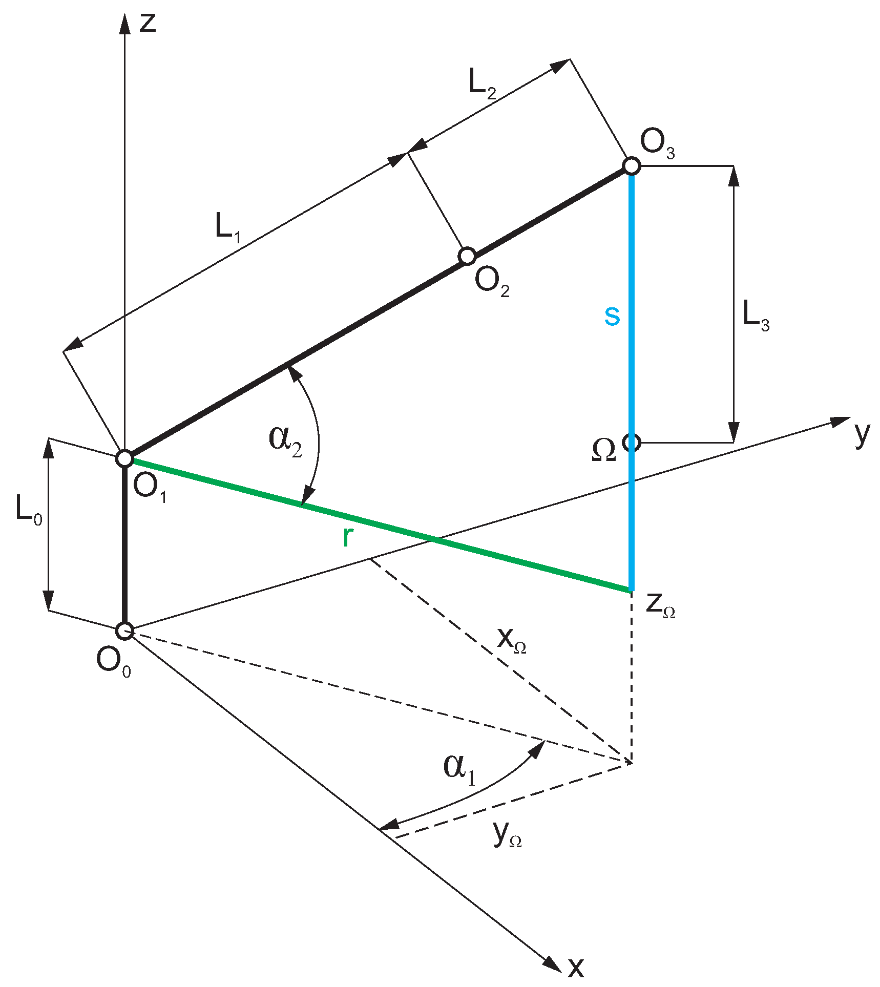
4. Inverse Kinematics Problem

In order to implement the movement of the load along the optimal trajectory in the crane, the problem of inverse kinematics must be solved, allowing for the determination of the functions controlling the individual parts of the device. The kinematic structure of the crane is shown in (Figure 12). The coordinates of the relevant articulations ( O 1 , O 2 , O 3 ) and the load suspension point ( Ω ) can be written as:
x 0 1 = 0 , y 0 1 = 0 , z 0 1 = L 0 ,
x 0 2 = L 1 cos α 2 cos α 1 , y 0 2 = L 1 cos α 2 sin α 1 , z 0 2 = L 0 + L 1 sin α 2 ,
x 0 3 = ( L 1 + L 2 ) cos α 2 cos α 1 , y 0 3 = ( L 1 + L 2 ) cos α 2 sin α 1 , z 0 3 = L 0 + ( L 1 + L 2 ) sin α 2 ,
x Ω = ( L 1 + L 2 ) cos α 2 cos α 1 , y Ω = ( L 1 + L 2 ) cos α 2 sin α 1 , z Ω = L 0 + ( L 1 + L 2 ) sin α 2 L 3 ,
where L 0 = c o n s t and L 1 = c o n s t .
The presented system is a redundant system, which means that no unique solution to the inverse kinematics problem can be obtained without imposing additional constraints. This feature increases the complexity of kinematic calculations and limits the practical applicability unless the problem is constrained by additional methods. To solve this problem, an algorithm of temporary restriction of movement of specific kinematic pairs [39] can be used. This method consists in locking one of the available degrees of freedom of the crane [40]. Due to the construction of the rotary crane, the best solution was to lock the last degree of freedom, i.e., the length of the rope ( L 3 = c o n s t ) remains constant during the entire duty cycle. Therefore, the crane is controlled by changing three parameters: platform rotation angle ( α 1 ), extension angle ( α 2 ) and cylinder extension length ( L 2 ). Although the simplification of keeping the rope length constant is commonly used in such models, it can potentially limit the ability to simulate more dynamic and realistic crane operations. In addition, the phenomenon of rope swinging was omitted—the rope ( O 3 Ω ) in the model is always parallel to the crane frame ( O 0 O 1 ). L 0 , L 1 , L 3 were assumed as constants.
Parameters s and r are described by relations:
r = x Ω 2 + y Ω 2 ,
s = z Ω L 0 + L 3 .
With such assumptions, it becomes possible to determine the values of the angles and the lengths of the members regardless of the coordinates of the Ω point. The only condition that the coordinates must meet is related to the construction of a crane (angle α 1 must be in the range 0 ÷ 270°, angle α 2 must be in the range 0 ÷ 60°, and the length L 2 in the range 0 ÷ 450 mm). The value of the angles α 1 and α 2 can be determined using the 2-argument arctangent function (atan2):
α 1 = a t a n 2 ( y Ω , z Ω ) , α 2 = a t a n 2 ( r , s ) ,
and calculate the length of L 2 from the following dependence:
L 2 = r 2 + s 2 L 1 .
The exemplary results of the numerical calculations show the change in the cylinder length L 2 (Figure 13), the angle of rotation of the platform (Figure 14) and the angle of change in the overhang α 2 (Figure 15) so that the duty cycle coincides with the minimum trajectory determined using algorithms. The obtained results are shown for the best solutions of the genetic algorithm and PSO. The following values were adopted in the simulations:
  • L 0 = 735 mm—distance from the ground to the place where the boom cylinder is attached,
  • L 1 = 710 mm—length of the first aluminum profile in which the actuator body is located,
  • L 3 = 735 mm—constant length of the rope, taking into account the height of the carried load (distance from the end of the boom to the lowest point of the carried load).
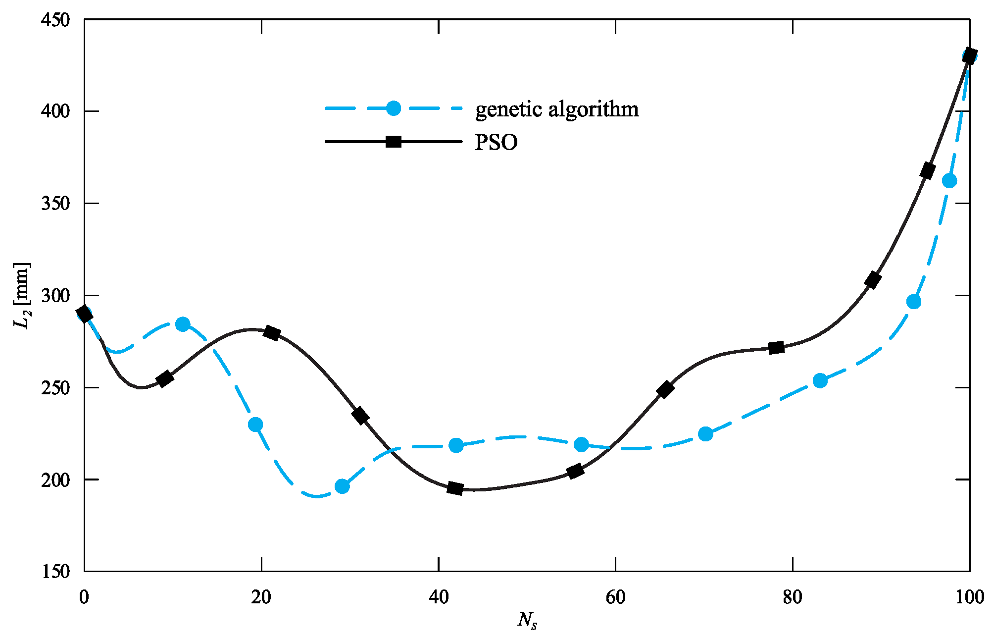
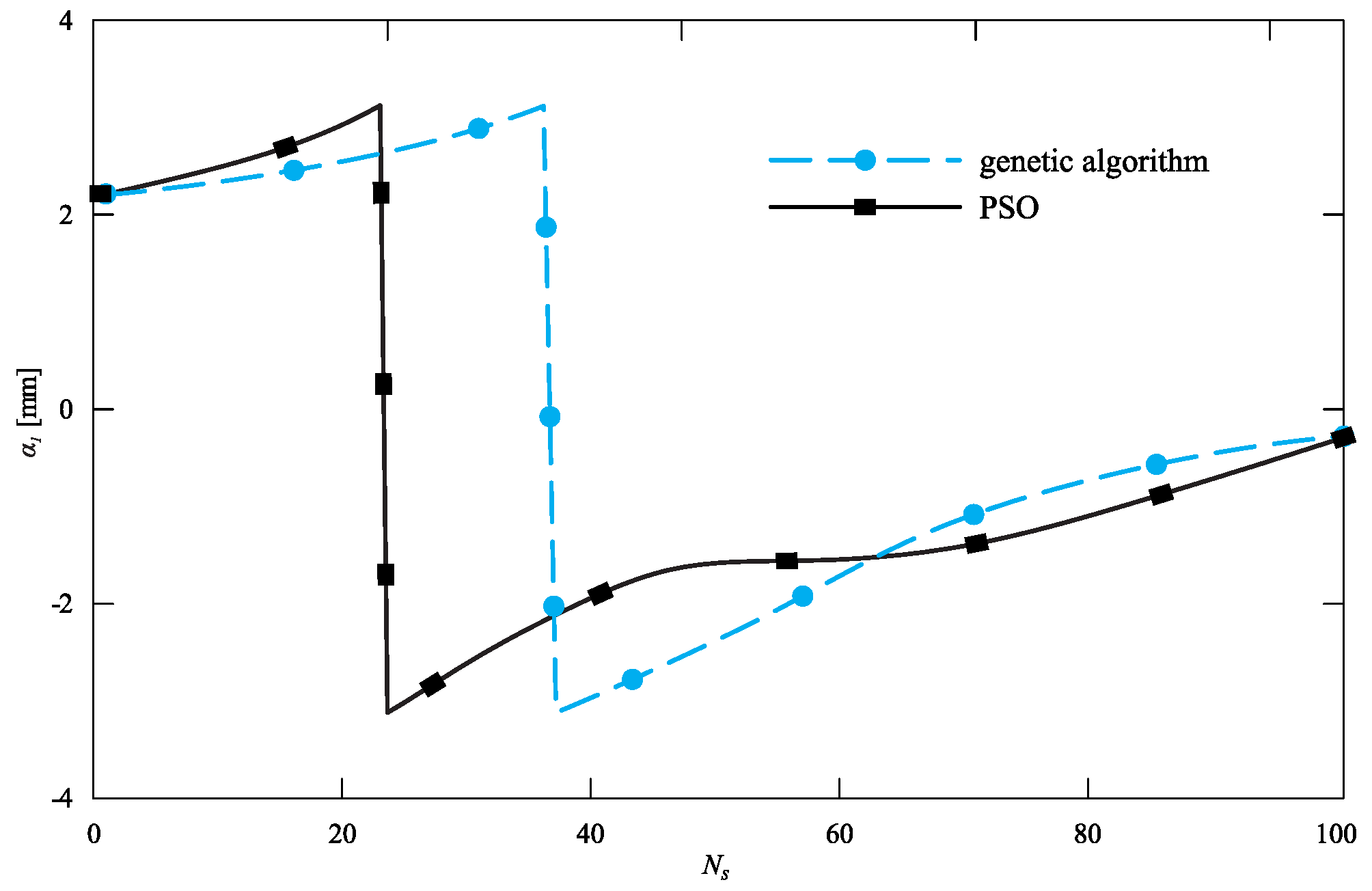
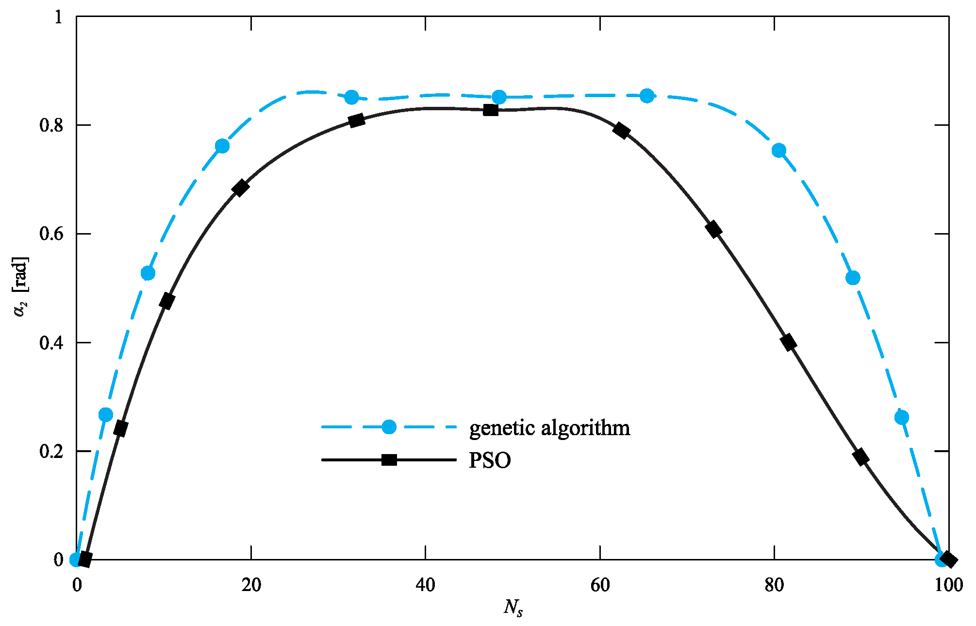
5. Discussion

From the obtained results, it can be seen that the determined solutions of inverse kinematics agree with the specified trajectories. Changes in length L 2 and angle α 2 are the smallest for the optimal trajectory ( l p o p = 50 ). The α 2 angle reached the maximum value for the l p o p = 30 variant, while the l p o p = 40 variant included the operation of the crane with the most extended actuator. The position in which the actuator is in the most retracted position was obtained for the population number of 50. Based on the obtained results, it can be concluded that due to the operation safety criterion, more favorable results were obtained for the PSO algorithm. Both the boom length ( L 2 ) and tilt angle change ( α 2 ) have been optimized to minimize the load on the crane actuators, indicating that PSO not only improves the performance but also increases the overall operational safety and service life of the crane components. Both the length of the boom ( L 2 ) and the change in inclination angle ( α 2 ) are smaller than those obtained using the genetic algorithm. As a result, the crane’s actuators will be less loaded, and ultimately, the maximum lifting capacity of the transporting machine will be increased.
Comparing the obtained results of optimization studies, a similar trend can be observed in other works presented in the literature. The effectiveness of PSO in minimizing the trajectory and computation time has been confirmed in studies such as [41], where the PSO algorithm found the optimal path with a shorter computation time. This is consistent with the results in this paper, reinforcing PSO as a more efficient choice for dynamic optimization tasks. In [41], as in the case of our work, it was found that the PSO algorithm found the optimal path in less computation time. A similar tendency can be found in [42]. As the number of iterations increases, the difference in simulation time between these algorithms increases in favor of PSO. In the case of [43], better results of the optimized function for GA than PSO were noted, but the differences in this article are larger than those obtained in this article. In [44], however, it was stated that in the case of a small scale of research, these algorithms can be used interchangeably, which confirms the results presented in the previous sections.

6. Conclusions

This paper presents the problem of optimizing the duty cycle of a rotary crane. Optimization was performed using the genetic and the PSO algorithm. As an objective function, minimization of the trajectory of the carried load was selected. Numerical simulations were performed for various parameters of the analyzed algorithms. On the basis of the shortest trajectory obtained, the position kinematics and the orientation of the crane members during the duty cycle were determined by solving the inverse kinematics problem. This task was solved using the geometric method and the algorithm for temporarily limiting the movement of specific kinematic pairs. Due to the structure of the crane, the movement of the last member was limited, i.e., the length of the rope remained constant.
The shortest trajectory during numerical simulations was obtained for the following parameters of the PSO algorithm: population number = 50, number of auxiliary points = 5, and the number of iterations in the range from 75 to 100. The presented algorithm works best for a larger number of auxiliary points (i = 5) and iterations ( i t > 75). In this case, the computation time is extended (even four times) in relation to a smaller number of iterations or auxiliary points. Increasing the number of populations also increases the computational time, but a shorter trajectory can be obtained as a result. For optimization studies, especially those involving more complex environments, using more auxiliary points and iterations would significantly improve the precision of the solution, although at the cost of increased computational time. This balance between accuracy and time efficiency is crucial when applying these methods to real lifting operations. For optimization tests similar to those presented in this paper, increasing the parameters of the PSO algorithm will lead to obtaining more favorable results with a slight increase in the computation time. On the other hand, for studies with a much greater degree of complexity, increasing the parameters of the PSO algorithm will result in a significant increase in the computation time while improving the obtained results by several percent. One of the most important parameters of the particle swarm algorithm is the number of auxiliary points. In the case presented in this work (when the working area is limited by three obstacles), it is advisable to use the same or more auxiliary points than the number of obstacles. If this condition is not met, the trajectory course differs significantly from the optimal trajectory, which is related to the construction of the B-spline curve.
The optimal trajectory obtained using the genetic algorithm was only 2 mm shorter compared to that determined using the PSO algorithm. This small difference suggests that both algorithms can be used interchangeably in applications where small deviations are acceptable. However, in industrial contexts where computational efficiency is crucial, the PSO algorithm has a significant advantage. Therefore, it can be concluded that during optimization tests concerning the minimization of the load trajectory, it is possible to use both methods, because the results obtained from their use do not differ significantly from each other. The only advantage of the PSO algorithm in this case is the shorter calculation time of the optimal trajectory. Among the parameters of the genetic algorithm, the probability of mutation and the population number have the greatest influence on obtaining the shortest path.
The obtained solution of inverse kinematics allows for determining the configuration coordinates for each point in the working area of the machine. In the analyzed case, it was found that the crane is able to reach all positions for the trajectory determined in the optimization process. Furthermore, the efficiency gains achieved with inverse kinematic solutions have direct implications for extending the crane’s operational reach while reducing mechanical stress. This improvement in mechanical efficiency can lead to greater crane lifting capacity and safer operation at higher loads. Finding the optimal trajectory resulted in a decrease in the coordinates of the change in the inclination angle α 2 , which has a fundamental impact on the crane’s duty cycle. If the angle increases and the cylinder extension remains in the extended position, the permissible crane capacity also decreases. If the optimal trajectory is achieved, the crane’s lifting capacity has also been increased, which means that the crane works with a lower load. For the algorithms adopted in the work, it was found that the PSO algorithm is a more advantageous approach when optimizing the crane’s duty cycle, due to the time of the calculations and the designated trajectory, which made it possible to relieve the machine’s drives.
Future work could extend these findings by integrating more dynamic crane behaviors, such as rope sway and environmental factors, into the optimization process. It is also planned to investigate hybrid algorithms combining PSO and GA to combine their respective strengths and achieve more efficient optimal solution finding. Additionally, future research could consider multi-objective optimization, extending the current methodology to aspects such as energy consumption or crane component operation, which would increase the generalizability of the results beyond the single-objective objective of trajectory length. Further research will also analyze the impact of baseline control scenarios to better understand the extent to which different optimization algorithms improve operational efficiency compared to more intuitive methods. This work will be further developed by taking into account the factors resulting from the crane dynamics in the mathematical model, taking into account the phenomenon of rope swinging in the inverse kinematics task, and solving the redundant system in a way that allows one to control all crane members.

Author Contributions

Conceptualization, D.C. and Z.P.; methodology, P.K. and D.S.; software, D.S., D.C. and P.K.; validation, P.K. and M.Š.; formal analysis, P.K.; investigation, P.K., D.S. and D.C.; resources, D.C.; data curation, P.K., D.S., D.C. and M.Š.; writing—original draft preparation, P.K. and D.C.; writing—review and editing, P.K., M.Š. and Z.P.; visualization, P.K., Z.P. and M.Š.; supervision, D.C.; project administration, D.C.; funding acquisition, D.C. All authors have read and agreed to the published version of the manuscript.

Funding

This research received no external funding.

Institutional Review Board Statement

Not applicable.

Informed Consent Statement

Not applicable.

Data Availability Statement

The data presented in this study are available upon request from the corresponding author. The data are not publicly available due to privacy restrictions.

Acknowledgments

The work was carried out as part of statutory research at the Department of Mechanics and Machine Design Fundamentals of the Czestochowa University of Technology.

Conflicts of Interest

The authors declare no conflicts of interest.

Abbreviations

The following abbreviations are used in this manuscript:
GAGenetic algorithm
PSOParticle Swarm Optimization
AGVAutomated guided vehicle
BIMBuilding Information Modeling
GWOGrey Wolf Optimizer
POPuma Optimizer
SASimulated annealing
CSCuckoo search

References

  1. Chwastek, S. Optimization of crane mechanisms to reduce vibration. Autom. Constr. 2020, 119, 103335. [Google Scholar] [CrossRef]
  2. Ermis, K.; Caliskan, M.; Tanriverdi, M. Design optimization of moveable moment stabilization system for access crane platforms. Acta Polytech. 2021, 61, 219–229. [Google Scholar] [CrossRef]
  3. Peng, B.; Flager, F.L.; Wu, J. A method to optimize mobile crane and crew interactions to minimize construction cost and time. Autom. Constr. 2018, 95, 10–19. [Google Scholar] [CrossRef]
  4. Yue, L.; Fan, H.; Zhai, C. Joint configuration and scheduling optimization of the dual trolley quay crane and AGV for automated container terminal. J. Phys. Conf. Ser. 2020, 1486, 072080. [Google Scholar] [CrossRef]
  5. Brzozowski, K.; Maczyński, A. Genetic algorithm in the task of load positioning in the rotation of the crane. Autobusy Tech. Eksploat. Syst. Transp. 2013, 14, 1403–1410. (In Polish) [Google Scholar]
  6. Hop, D.C.; Hop, N.V.; Anh, T.T.M. Adaptive particle swarm optimization for integrated quay crane and yard truck scheduling problem. Comput. Ind. Eng. 2021, 153, 107075. [Google Scholar] [CrossRef]
  7. Pan, Z.; Guo, H.; Li, Y. Automated Method for Optimizing Feasible Locations of Mobile Cranes Based on 3D Visualization. Procedia Eng. 2017, 196, 36–44. [Google Scholar] [CrossRef]
  8. Riga, K.; Jahr, K.; Thielen, C.; Borrmann, A. Mixed integer programming for dynamic tower crane and storage area optimization on construction sites. Autom. Constr. 2020, 120, 103259. [Google Scholar] [CrossRef]
  9. Farrage, A.; Takahashi, H.; Terauchi, K.; Sasai, S.; Sakurai, H.; Okubo, M.; Uchiyama, N. Modified A* Algorithm for Optimal Motion Trajectory Generation of Rotary Cranes. In Proceedings of the 2023 IEEE International Conference on Mechatronics (ICM), Loughborough, UK, 15–17 March 2023; IEEE: Piscataway, NJ, USA, 2023; Volume 39, pp. 1–6. [Google Scholar] [CrossRef]
  10. Zhao, Y.; Zhu, Y.; Zhang, P.; Gao, Q.; Han, X. A Hybrid A* Path Planning Algorithm Based on Multi-objective Constraints. In Proceedings of the 2022 Asia Conference on Advanced Robotics, Automation, and Control Engineering (ARACE), Qingdao, China, 26–28 August 2022; IEEE: Piscataway, NJ, USA, 2022; Volume 152, pp. 1–6. [Google Scholar] [CrossRef]
  11. Hameed, I.A.; Bye, R.T.; Osen, O.L. Grey wolf optimizer (GWO) for automated offshore crane design. In Proceedings of the 2016 IEEE Symposium Series on Computational Intelligence (SSCI), Athens, Greece, 6–9 December 2016; IEEE: Piscataway, NJ, USA, 2016. [Google Scholar] [CrossRef]
  12. Abdollahzadeh, B.; Khodadadi, N.; Barshandeh, S.; Trojovský, P.; Gharehchopogh, F.S.; El-kenawy, E.S.M.; Abualigah, L.; Mirjalili, S. Puma optimizer (PO): A novel metaheuristic optimization algorithm and its application in machine learning. Clust. Comput. 2024, 27, 5235–5283. [Google Scholar] [CrossRef]
  13. Kim, Y.; Kim, T.; Lee, H. Heuristic algorithm for retrieving containers. Comput. Ind. Eng. 2016, 101, 352–360. [Google Scholar] [CrossRef]
  14. Cai, P.; Cai, Y.; Chandrasekaran, I.; Zheng, J. Parallel genetic algorithm based automatic path planning for crane lifting in complex environments. Autom. Constr. 2016, 62, 133–147. [Google Scholar] [CrossRef]
  15. Bertolini, M.; Esposito, G.; Mezzogori, D.; Neroni, M. Optimizing Retrieving Performance of an Automated Warehouse for Unconventional Stock Keeping Units. Procedia Manuf. 2019, 39, 1681–1690. [Google Scholar] [CrossRef]
  16. Xiang, G.; Xiang, X. 3D trajectory optimization of the slender body freely falling through water using cuckoo search algorithm. Ocean Eng. 2021, 235, 109354. [Google Scholar] [CrossRef]
  17. Haghighi, H.; Sadati, S.H.; Dehghan, S.M.; Karimi, J. Hybrid Form of Particle Swarm Optimization and Genetic Algorithm For Optimal Path Planning in Coverage Mission by Cooperated Unmanned Aerial Vehicles. J. Aerosp. Technol. Manag. 2020, 12, e4320. [Google Scholar] [CrossRef]
  18. Betts, J.T. Survey of Numerical Methods for Trajectory Optimization. J. Guid. Control Dyn. 1998, 21, 193–207. [Google Scholar] [CrossRef]
  19. Ratiu, M.; Prichici, M.A. Industrial robot trajectory optimization- a review. MATEC Web Conf. 2017, 126, 02005. [Google Scholar] [CrossRef]
  20. Shirazi, A.; Ceberio, J.; Lozano, J.A. Spacecraft trajectory optimization: A review of models, objectives, approaches and solutions. Prog. Aerosp. Sci. 2018, 102, 76–98. [Google Scholar] [CrossRef]
  21. Yan, T.; Lu, F.; Wang, S.; Wang, L.; Bi, H. A hybrid metaheuristic algorithm for the multi-objective location-routing problem in the early post-disaster stage. J. Ind. Manag. Optim. 2023, 19, 4663–4691. [Google Scholar] [CrossRef]
  22. Lu, F.; Jiang, R.; Bi, H.; Gao, Z. Order Distribution and Routing Optimization for Takeout Delivery under Drone–Rider Joint Delivery Mode. J. Theor. Appl. Electron. Commer. Res. 2024, 19, 774–796. [Google Scholar] [CrossRef]
  23. Liu, D.; Deng, Z.; Mao, X.; Yang, Y.; Kaisar, E.I. Two-Echelon Vehicle-Routing Problem: Optimization of Autonomous Delivery Vehicle-Assisted E-Grocery Distribution. IEEE Access 2020, 8, 108705–108719. [Google Scholar] [CrossRef]
  24. Guo, J.; Chen, L.; Tang, B.; Gen, M. Optimal strategies for an uncertain forward and reverse multi-period logistics network using heuristic algorithm: A case study of Shanghai perishable products. Int. J. Internet Manuf. Serv. 2024, 10, 132–164. [Google Scholar] [CrossRef]
  25. Kwiatoń, P. Modeling and Dynamics Studies, Stability Analysis and Optimization of the Duty Cycle of a Mobile Crane. Ph.D. Thesis, Czestochowa University of Technology, Częstochowa, Poland, 2021. (In Polish). [Google Scholar]
  26. Skrobek, D. Modeling, Analysis and Optimization of the Duty Cycle of Manipulators with Four Degrees of Freedom. Ph.D. Thesis, Czestochowa University of Technology, Częstochowa, Poland, 2019. (In Polish). [Google Scholar]
  27. Cekus, D.; Depta, F.; Kubanek, M.; Kuczyński, Ł.; Kwiatoń, P. Event Visualization and Trajectory Tracking of the Load Carried by Rotary Crane. Sensors 2022, 22, 480. [Google Scholar] [CrossRef] [PubMed]
  28. Jordehi, A.R. A review on constraint handling strategies in particle swarm optimisation. Neural. Comput. Appl. 2015, 26, 1265–1275. [Google Scholar] [CrossRef]
  29. Gupta, R.; Bhunia, A.; Roy, D. A GA based penalty function technique for solving constrained redundancy allocation problem of series system with interval valued reliability of components. J. Comput. Appl. Math. 2009, 232, 275–284. [Google Scholar] [CrossRef]
  30. Cekus, D.; Kwiatoń, P.; Šofer, M.; Šofer, P. Application of heuristic methods to the identification of the parameters of discrete-continuous models. Bull. Pol. Acad. Sci. Tech. Sci. 2022, 70, e140150. [Google Scholar] [CrossRef]
  31. Kennedy, J.; Eberhart, R. Particle swarm optimization. In Proceedings of the ICNN’95—International Conference on Neural Networks, Perth, Australia, 27 November–1 December 1995; IEEE: Piscataway, NJ, USA, 1995. [Google Scholar] [CrossRef]
  32. Cekus, D.; Skrobek, D. The influence of inertia weight on the particle swarm optimization algorithm. J. Appl. Math. Comput. Mech. 2018, 17, 5–11. [Google Scholar] [CrossRef]
  33. Herlambang, T.; Rahmalia, D.; Yulianto, T. Particle Swarm Optimization (PSO) and Ant Colony Optimization (ACO) for optimizing PID parameters on Autonomous Underwater Vehicle (AUV) control system. J. Phys. Conf. Ser. 2019, 1211, 012039. [Google Scholar] [CrossRef]
  34. Taherkhani, M.; Safabakhsh, R. A novel stability-based adaptive inertia weight for particle swarm optimization. Appl. Soft Comput. 2016, 38, 281–295. [Google Scholar] [CrossRef]
  35. Xu, G. An adaptive parameter tuning of particle swarm optimization algorithm. Appl. Math. Comput. 2013, 219, 4560–4569. [Google Scholar] [CrossRef]
  36. Liu, Q.; Wei, W.; Yuan, H.; Zhan, Z.H.; Li, Y. Topology selection for particle swarm optimization. Inf. Sci. 2016, 363, 154–173. [Google Scholar] [CrossRef]
  37. Jordehi, A.R.; Jasni, J. Parameter selection in particle swarm optimisation: A survey. J. Exp. Theor. Artif. Intell. 2013, 25, 527–542. [Google Scholar] [CrossRef]
  38. Skrobek, D.; Cekus, D. Optimization of the operation of the anthropomorphic manipulator in a three-dimensional working space. Eng. Opt. 2019, 51, 1997–2010. [Google Scholar] [CrossRef]
  39. Herebin, P.; Pajor, M. Modeling the simple and inverse kinematics of a truck crane with a redundant structure using the MATLAB environment (in Polish). Eng. Model. 2016, 58, 44–50. [Google Scholar]
  40. D’Souza, A.; Vijayakumar, S.; Schaal, S. Learning inverse kinematics. In Proceedings of the 2001 IEEE/RSJ International Conference on Intelligent Robots and Systems. Expanding the Societal Role of Robotics in the the Next Millennium (Cat. No.01CH37180), Maui, HI, USA, 29 October–3 November 2001; IEEE: Piscataway, NJ, USA, 2001. [Google Scholar] [CrossRef]
  41. Sooda, K.; Nair, T. A Comparative Analysis for Determining the Optimal Path using PSO and GA. Int. J. Comput. Appl. 2011, 32, 8–12. [Google Scholar]
  42. Khoshahval, F.; Minuchehr, H.; Zolfaghari, A. Performance evaluation of PSO and GA in PWR core loading pattern optimization. Nucl. Eng. Des. 2011, 241, 799–808. [Google Scholar] [CrossRef]
  43. Alaia, E.B.; Harbaoui, I.; Borne, P.; Bouchriha, H. A Comparative Study of the PSO and GA for the m-MDPDPTW. Int. J. Comput. Commun. Control. 2018, 13, 8. [Google Scholar] [CrossRef]
  44. Wihartiko, F.D.; Wijayanti, H.; Virgantari, F. Performance comparison of genetic algorithms and particle swarm optimization for model integer programming bus timetabling problem. IOP Conf. Ser. Mater. Sci. Eng. 2018, 332, 012020. [Google Scholar] [CrossRef]
Figure 1. Rotary crane working environment.
Applsci 14 09940 g001
Figure 2. Scheme of the genetic algorithm.
Applsci 14 09940 g002
Figure 3. The course of the convergence function of the genetic algorithm.
Applsci 14 09940 g003
Figure 4. Scheme of the particle swarm optimization algorithm.
Applsci 14 09940 g004
Figure 5. The course of the convergence function of the PSO algorithm.
Applsci 14 09940 g005
Figure 6. Projection of the shortest trajectories onto the XY plane for different population values.
Applsci 14 09940 g006
Figure 7. Projection of the shortest trajectories onto the XZ plane for different population values.
Applsci 14 09940 g007
Figure 8. Projection of the shortest trajectories onto the YZ plane for different population values.
Applsci 14 09940 g008
Figure 9. Projection of the shortest trajectories onto the XY plane for various auxiliary points.
Applsci 14 09940 g009
Figure 10. Projection of the shortest trajectories onto the XZ plane for various auxiliary points.
Applsci 14 09940 g010
Figure 11. Projection of the shortest trajectories onto the YZ plane for various auxiliary points.
Applsci 14 09940 g011
Figure 12. Kinematic diagram of the crane with marked values r and s.
Applsci 14 09940 g012
Figure 13. Change in the length of L 2 for the shortest trajectory of the algorithms.
Applsci 14 09940 g013
Figure 14. Change in the α 1 angle for the shortest of the determined trajectories of the algorithms.
Applsci 14 09940 g014
Figure 15. Change in the α 2 angle for the shortest of the determined trajectories of the algorithms.
Applsci 14 09940 g015
Table 1. Value of the objective function and computation time for various parameters of the genetic algorithm— p k = 0.5 and p m = 0.1 .
ItPopulation Number l pop
50 100
Number of Waypoints
8101281012
500L [mm]361839623900365138164010
T [s]70.876.584.4151.6157.3164.7
1000L [mm]361337433875356437853849
T [s]143.2156.5185.6307.3297.1312.7
Table 2. Value of the objective function and computation time for various parameters of the genetic algorithm— p k = 0.8 and p m = 0.05 .
ItPopulation Number l pop
50 100
Number of Waypoints
8101281012
500L [mm]375439103962361936103659
T [s]73.680.886.5147.9164.5180.4
1000L [mm]366037763760363036523841
T [s]143.6159.4177.9292.7320.8359.3
Table 3. Value of the objective function (trajectory L) and calculation time for various parameters of the genetic algorithm— p k = 0.8 and p m = 0.1 .
ItPopulation Number l pop
50 100
Number of Waypoints
8101281012
500L [mm]361738683729380336153814
T [s]86.681.287.8150.4169.2183.1
1000L [mm]359837183690368235893777
T [s]161.4179.3176.6299.2330.8361.7
Table 4. Value of the objective function (trajectory L) and calculation time for various parameters of the genetic algorithm— p k = 0.5 and p m = 0.05 .
ItPopulation Number l pop
50 100
Number of Waypoints
8101281012
500L [mm]367638303801357937883738
T [s]73.479.183.0142.9154.8167.9
1000L [mm]374236783853367837033817
T [s]153.5153.3167.7281.7317.5343.3
Table 5. Value of the objective function and calculation time for various parameters of the PSO algorithm— l p o p = 20 .
Population Number l pop = 20
It Number of Auxiliary Points
i = 2i = 3i = 4i = 5
L
[mm]
T
[s]
L
[mm]
T
[s]
L
[mm]
T
[s]
L
[mm]
T
[s]
2539185.238475.338825.137775.4
5039219.537339.838099.9367710.2
75391214.4377415.0381014.5369815.0
100385218.5370419.5382119.1363819.8
Table 6. Value of the objective function and calculation time for various parameters of the PSO algorithm— l p o p = 30 .
Population Number l pop = 30
It Number of Auxiliary Points
i = 2i = 3i = 4i = 5
L
[mm]
T
[s]
L
[mm]
T
[s]
L
[mm]
T
[s]
L
[mm]
T
[s]
2539296.236996.638976.438296.6
50386712.4367812.2384212.5374012.8
75389918.5364018.9376619.0365918.7
100390924.1367024.4370125.1362924.1
Table 7. Value of the objective function and calculation time for various parameters of the PSO algorithm— l p o p = 40 .
Population Number l pop = 40
It Number of Auxiliary Points
i = 2i = 3i = 4i = 5
L
[mm]
T
[s]
L
[mm]
T
[s]
L
[mm]
T
[s]
L
[mm]
T
[s]
2539327.837707.739058.037517.7
50387214.5362415.4373915.2370915.2
75390121.9370522.3382722.6360222.6
100386929.2369128.9377729.5358729.2
Table 8. Value of the objective function and calculation time for various parameters of the PSO algorithm— l p o p = 50 .
Population Number l pop = 50
ItNumber of Auxiliary Points
i = 2i = 3i = 4i = 5
L
[mm]
T
[s]
L
[mm]
T
[s]
L
[mm]
T
[s]
L
[mm]
T
[s]
2539209.436609.237979.537369.1
50393717.2369917.7375917.1363018.2
75391925.4362625.5375125.3356626.0
100389333.6368334.0371734.5359934.8
Disclaimer/Publisher’s Note: The statements, opinions and data contained in all publications are solely those of the individual author(s) and contributor(s) and not of MDPI and/or the editor(s). MDPI and/or the editor(s) disclaim responsibility for any injury to people or property resulting from any ideas, methods, instructions or products referred to in the content.

