Deep Learning-Based Low-Frequency Passive Acoustic Source Localization

Abstract

This paper develops benchmark cases for low- and very-low-frequency passive acoustic source localization (ASL) using synthetic data. These cases can be potentially applied to the detection of turbulence-generated low-frequency acoustic emissions in the atmosphere. A deep learning approach is used as an alternative to conventional beamforming, which performs poorly under these conditions. The cases, which include two- and three-dimensional ASL, use a shallow and inexpensive convolutional neural network (CNN) with an appropriate input feature to optimize the source localization. CNNs are trained on a limited dataset to highlight the computational tractability and viability of the low-frequency ASL approach. Despite the modest training sets and computational expense, detection accuracies of at least 80% and far superior performance compared with beamforming are achieved—a result that can be improved with more data, training, and deeper networks. These benchmark cases offer well-defined and repeatable representative problems for comparison and further development of deep learning-based low-frequency ASL.

1. Introduction

The detection of low-frequency acoustic sources is an important topic in the field of acoustic source localization (ASL). Low-frequency sources (30–300 Hz) and their detection are common in the fields of aeroacoustics, underwater acoustics [1,2,3], seismology [4,5,6], and other related fields [7]. Here, we are primarily interested in applications in aeroacoustics, specifically in the turbulence-generated low-frequency acoustic emissions. Wake turbulence, which is characterized by wake vortices, has been shown to emit a characteristic low-frequency noise [8] that can be used to locate wake vortices in an effort to minimize wake turbulence encounters [9] and increase airport efficiency and throughput [10]. Other applications include large-scale atmospheric turbulence detection [11] using ground-based microphone arrays and the characterization of volcano jets through their aeroacoustics information [12].

Acoustic sources at low frequencies cause methods such as conventional beamforming [13,14,15] to suffer from poor resolution. Figure 1 shows the increasingly poor localization predictions as the source frequency decreases. The resolution is even poorer for the low-frequency range we are interested in. This can be attributed to the Rayleigh resolution criterion, originally given for the angular resolution of an optical system [16] but can be applied analogously to an acoustical system. The source map obtained from conventional beamforming can be improved through post-processing by deconvolution algorithms such as DAMAS [17] and CLEAN-SC [14]; however, a perfectly clean and accurate source map is difficult to obtain [18]. Due to this limitation of beamforming, other approaches for low-frequency source localization have to be explored.

Machine learning (ML), and deep learning (DL) in particular, have shown great promise in the field of acoustics [20,21,22]. Deep learning algorithms involve the use of neural networks that process data in multiple layers to perform regression, classification, and many other such tasks.

Despite the limitations of these methods, such as requiring large numbers of data and not being physically intuitive, the ability of deep learning algorithms to extract features from data in any shape or form provides much scope for their application in ASL. Thus, the goal of this paper is to build deep learning models for low-frequency ASL as an alternative to beamforming.

A general study of the literature on deep learning-based ASL offers insights into the different kinds of input features and network architectures used, which can then be applied to low-frequency source localization. Most research in deep learning-based ASL is focused on the localization of speech signals. While most works process the acoustic data before feeding them to a network, Vera-Diaz et al. [23] were the first to use raw audio signals as input to a convolutional neural network (CNN) [24] to predict the position of the three-dimensional source. Chakrabarty and Habets [25] and Xiao et al. [26] used the phase component of the short-time Fourier transform (STFT) and Generalized Cross-Correlation with Phase Transform (GCC-PHAT), respectively, as input for estimating the direction of arrival (DoA) of speech signals.

Studies focusing on a source frequency range such as Ma and Liu [27] simulated a phased microphone array and monopole sources at high frequencies (3000–8000 Hz) on a scanning plane, and used the cross-spectral matrix (CSM) as input to a CNN for localization of these sources. They were able to demonstrate excellent spatial resolution, comparable to that of DAMAS, and much better than conventional beamforming. However, they did not address the challenges at lower source frequencies. Xu et al. [18] employed a similar setup and methodology, but focused on a wider source frequency range of 200–20,000 Hz and were able to predict the source distribution, even for low frequencies. However, they used a densely connected convolutional network (DenseNet) [28] that required large numbers of data and a large amount of memory for training. Niu et al. [29] carried out ocean source localization in the frequency range of 100–200 Hz using a single hydrophone and the discrete Fourier transform of the raw pressure data. Fifty-layer residual networks (ResNet-50), which also needed a significant number of training data, were separately trained to determine the range and depth of the source.

The literature has broadly explored the viability of deep learning techniques for low-frequency acoustic source localization. Most of it, however, does not focus exclusively on low-frequency sound, and infrasound (below 20 Hz). The works that do [18,30] use very deep and computationally expensive network architectures. Thus, in this paper, we present deep learning models for three reproducible test cases covering two-dimensional and three-dimensional ASL, as a proof-of-concept for the viability of deep learning methods exclusively in low- and very-low-frequency ASL. The models are built using limited data and computationally inexpensive networks. These test cases, which contain key features of applied ASL problems, seek to optimize low-frequency ASL under imposed computational limits and are intended to serve as benchmark cases for studying and further developing low-frequency ASL using deep learning. We adopted a relatively shallow CNN (fewer numbers of layers as compared with a deep neural network such as DenseNet), which was inexpensive and capable of being trained on limited data, for all the cases with an appropriate input feature. Section 2 gives a comprehensive description of the method. Section 3 provides the details of all test cases. Section 4 discusses the results obtained from the cases, followed by the conclusion.

2. Method

The methodology used for low-frequency ASL in this paper can be described in three steps. The first step involves collecting the synthetic acoustic pressure data using a simulated microphone array. These data are then processed, either in the time or frequency domain, to generate an input feature capable of being fed to a CNN. Finally, the CNN is trained with the generated input feature against the ground truth and is used to make predictions. The method is summarized in Figure 2.

Figure 3 shows a flowchart of the three test cases for low-frequency ASL developed in this paper. Case 1 (inspired by Xu et al. [18], Ma and Liu [27]) is regression-based two-dimensional ASL on a scanning plane parallel to the microphone array plane. This setup can be applied to the detection of aeroacoustic sources, such as wake vortices that emit low-frequency noise. Case 2 (source localization on the horizon), also two-dimensional, tackles ASL as a direction-of-arrival (DoA) estimation problem through a classification approach. Case 3, which is an extension of case 2, deals with three-dimensional ASL. Cases 2 and 3 are inspired by the work of Shams et al. [11] on the development of an early-warning clear-air turbulence (CAT) detection system using a ground-based microphone array. All the cases are discussed in detail in Section 3.

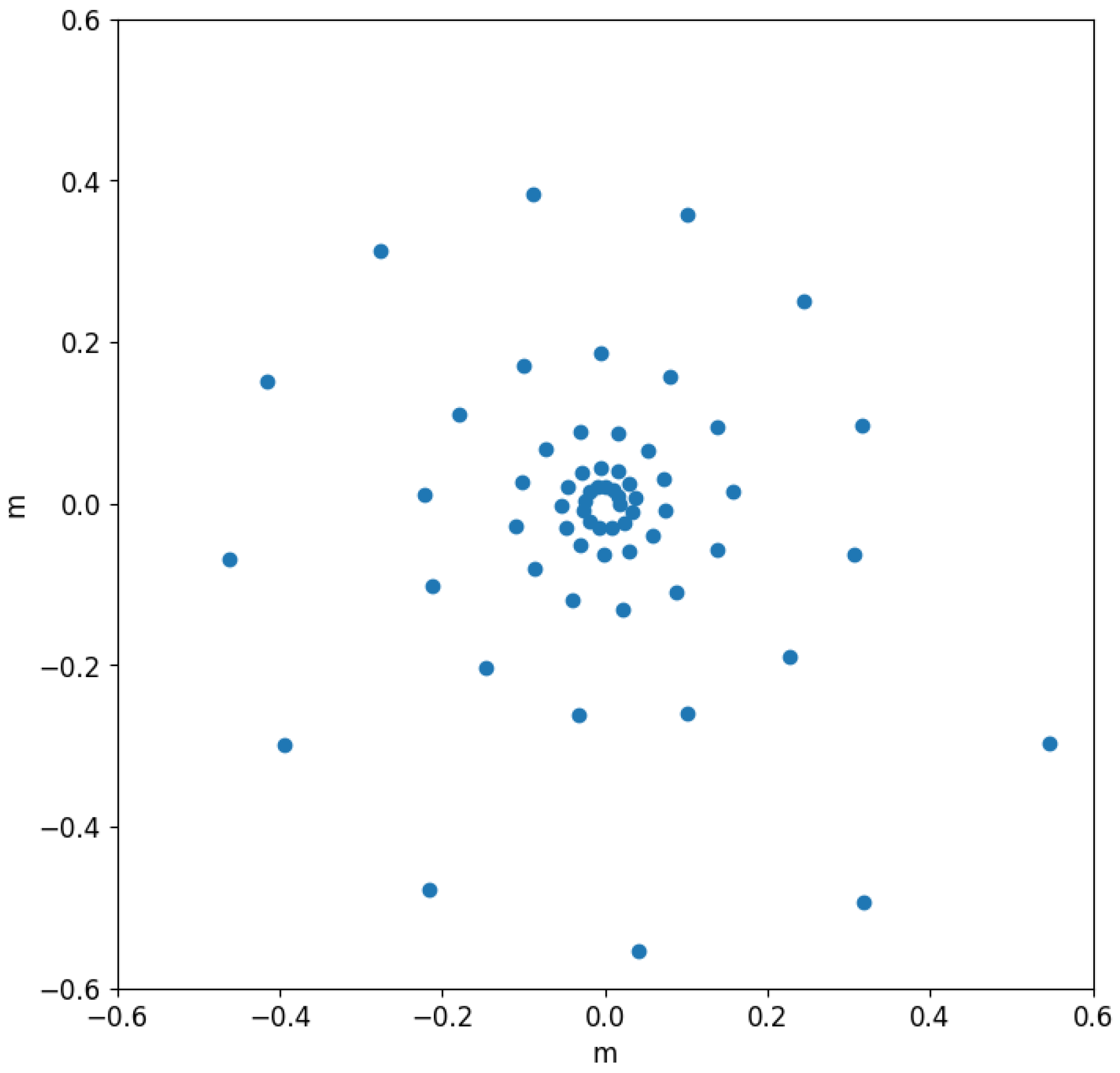
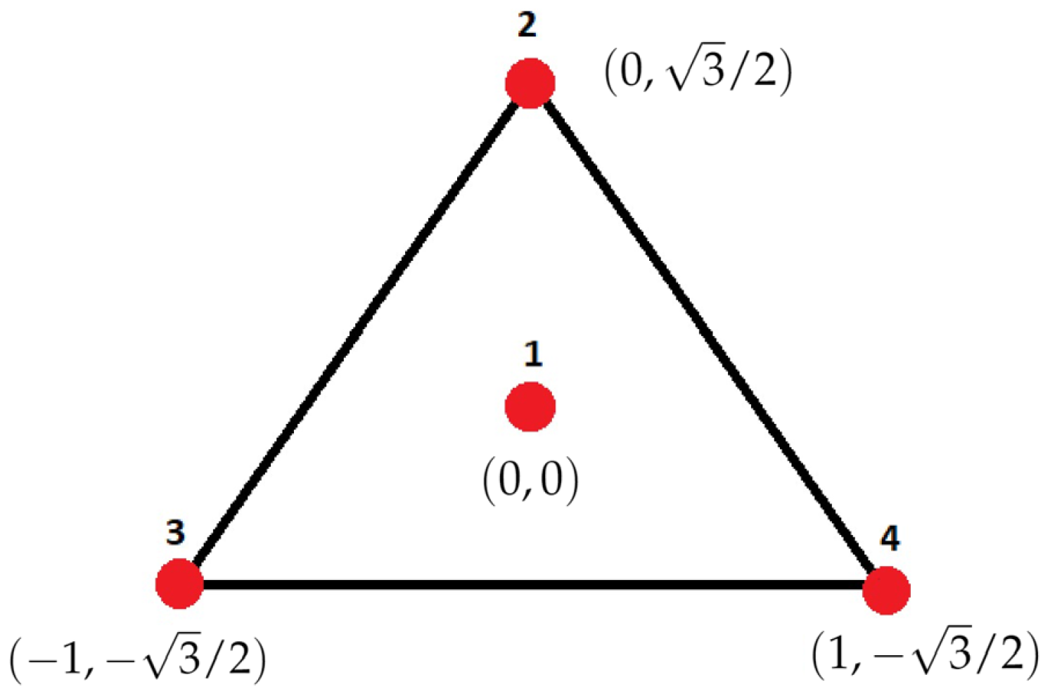
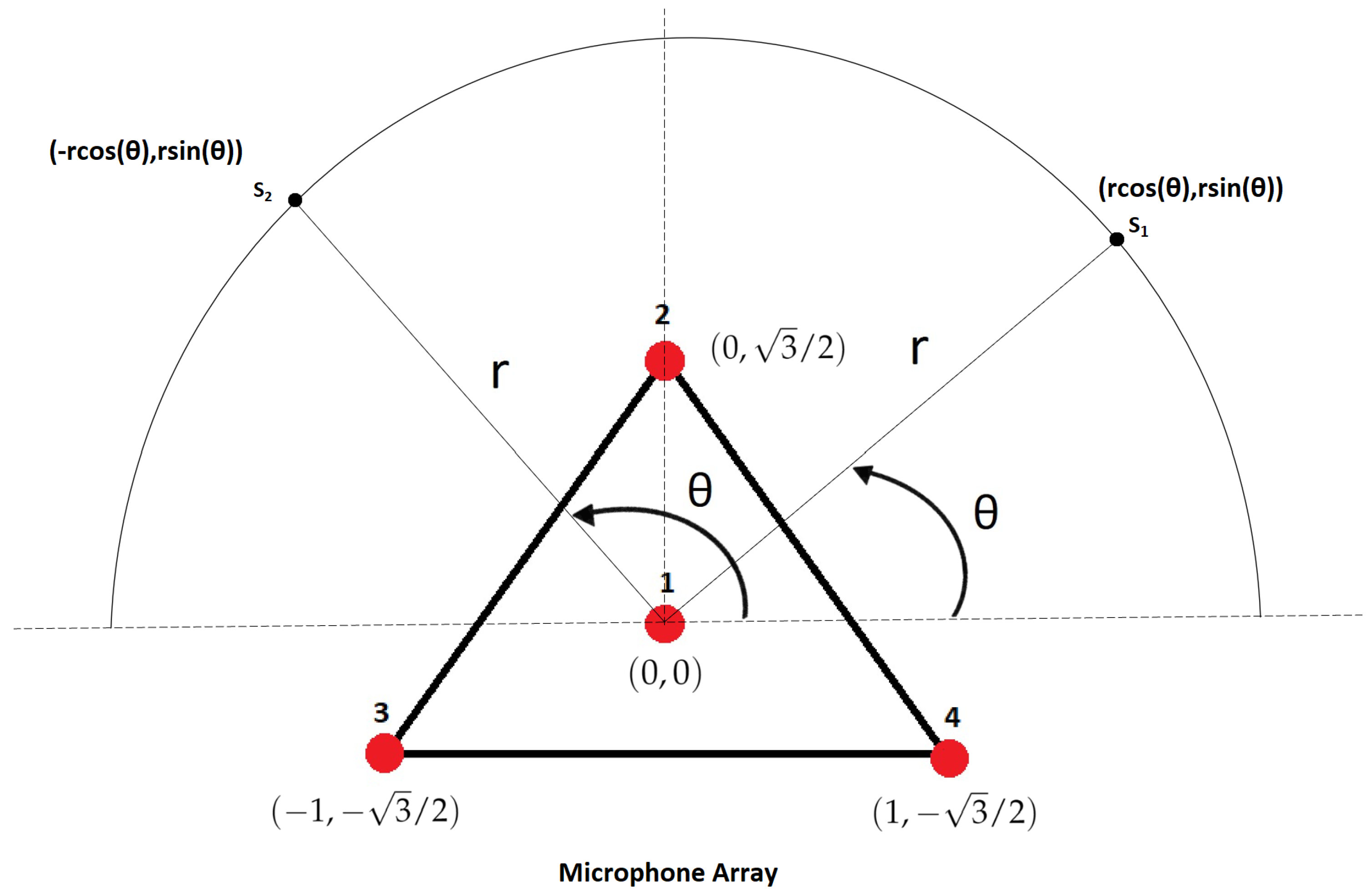
2.1. Microphone Array and Source Simulation

Two types of microphone arrays and sources are simulated. The first type of array, used for case 1, is a 64-microphone array in the shape of a logarithmic spiral. A spiral is naturally irregular and has unique inter-microphone spacing, which is needed to avoid spatial aliasing, thus making it a popular architecture for microphone arrays [31]. The specific type of logarithmic spiral used in this paper is called the Arcondoulis spiral, which performs well over a range of frequencies. The equation of the spiral is $r=a{e}^{b\theta }$, wherein the parameters a and b are set as $a=0.018$ and $b=0.002$ to obtain the microphone array as shown in Figure 4, similar to the array used by Xu et al. [18].

Using a large number of microphones may not always be economically viable nor is it necessary to capture low-frequency content, thus we also simulated a more minimalistic array. The microphone array used for cases 2 and 3 is a four-microphone array, as shown in Figure 5. The design is inspired by the triangular array used by Shams et al. [11]. The addition of a fourth microphone introduces variation in inter-microphone spacing and provides more data and a better-sized input feature to work with. The chosen array depends on whether the case is modeled as a regression or classification task. Case 1 is modeled as a regression problem to accurately predict the location of the sources. Due to its complexity, the array with more microphones is chosen. Cases 2 and 3 are classification tasks that involve estimating the DoA of the signal. They are relatively less complex and thus use the four-microphone array.

We simulated two types of sources with different levels of complexity. Source 1 (S1) (Equation (1)) is an analytically-defined monopole that oscillates at a fixed frequency, f. $P_s\left(m\right)$ (Equation (1)) shows the complex acoustic pressure due to a monopole, s, as detected by a microphone, m, located at a distance $r_s$ from the source. Here, Q is the complex source strength, and $c_0$ is the speed of sound in the air, both assumed to be constant. S1 exhibits geometric decay through distance-based attenuation of the complex pressure signal. It is computationally inexpensive and allows us to test models rapidly.

$$\begin{array}{c}\hfill P_s\left(m\right)=Q{\displaystyle \frac{e^{-j2\pi f{r}_s/c_o}}{4\pi |r_s|}}\end{array}$$

(1)

The second type of source, source 2 (S2) (Equation (2)), is also an analytical source: a time-domain sinusoidal plane wave of amplitude A, frequency f, and phase difference $\varphi$. The phase difference for one microphone with respect to another is given in terms of the time delay ($\Delta t$) in the signal received by the pair of microphones. The plane wave signal is defined at the microphone location, which is fixed, and thus varies sinusoidally with time. The signal is polluted with noise that can be correlated, uncorrelated noise, or a combination of both:

$$\begin{array}{cc}\hfill & P\left(t\right)=Asin(2\pi ft+\varphi )+\mathit{Noise}\hfill \end{array}$$

(2)

where $\varphi =2\pi f\Delta t$. Being a plane wave, S2 does not undergo any geometric or viscous decay. Unlike S1, which is strictly defined in the frequency domain, S2 can be used for both time- and frequency-domain processing.

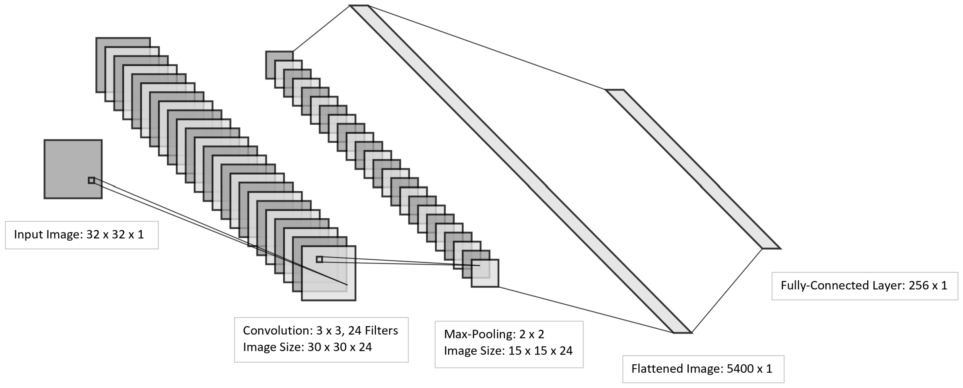
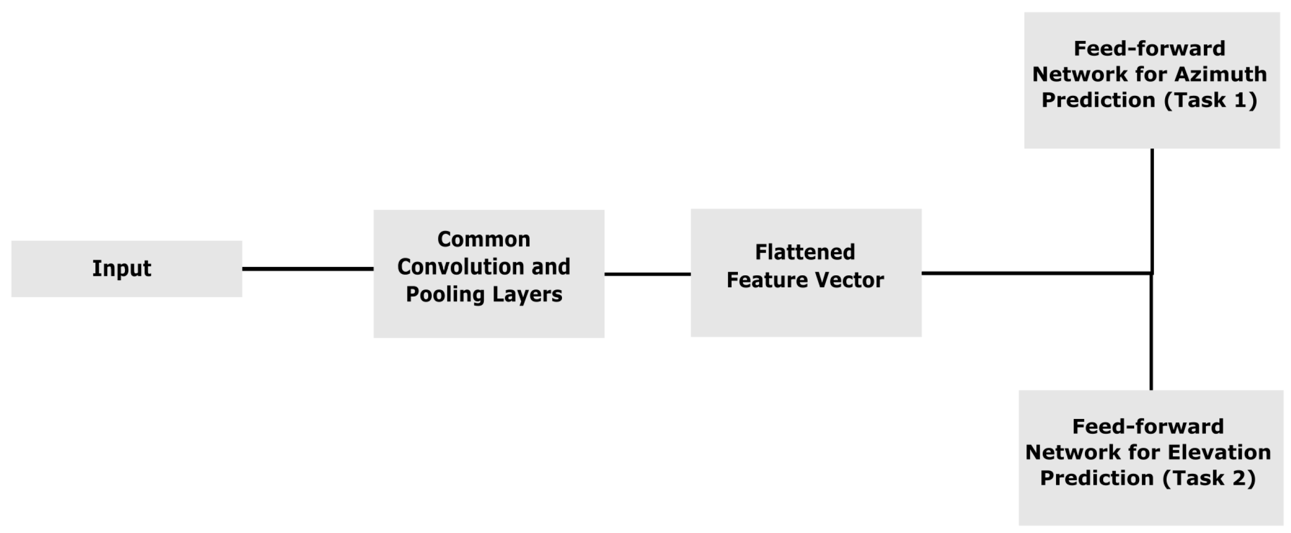
2.2. Convolutional Neural Network

A shallow convolutional neural network (CNN) similar to the generic network shown in Figure 6 is adopted for all cases in this paper. Figure 6 shows the working of a CNN through convolution and pooling operations performed on a $32\times 32\times 1$ image. The stride values for the convolution and pooling layers are 1 and 2, respectively. Once the image is fed to the CNN, the convolution layer applies a series of filters to help the network capture the various characteristics of the image. The image size thus changes after the convolution operation. For an image of dimensions $I\times I$, filter width $F\times F$, zero-padding P, and stride S, the output dimensions of the image are $\left[{\displaystyle \frac{(I-F+2P)}{S}}+1\right]\times \left[{\displaystyle \frac{(I-F+2P)}{S}}+1\right]$ [32]. This is followed by a pooling layer that downsamples the image, thereby reducing its size while preserving the dominant features. The dimensions of an $I\times I$ image after a $F\times F$ max-pooling filter operation are $\left[{\displaystyle \frac{(I-F)}{S}}+1\right]\times \left[{\displaystyle \frac{(I-F)}{S}}+1\right]$. The resulting image is flattened to a vector and fed to a fully connected layer as part of a regular feed-forward network. The loss and activation functions in the final layer are chosen depending on the nature of the case, i.e., whether it is a regression problem or a classification problem. The CNN compares its prediction with the ground truth, calculates the loss/error, and adjusts its learnable parameters to minimize the loss.

3. Test Case Setups

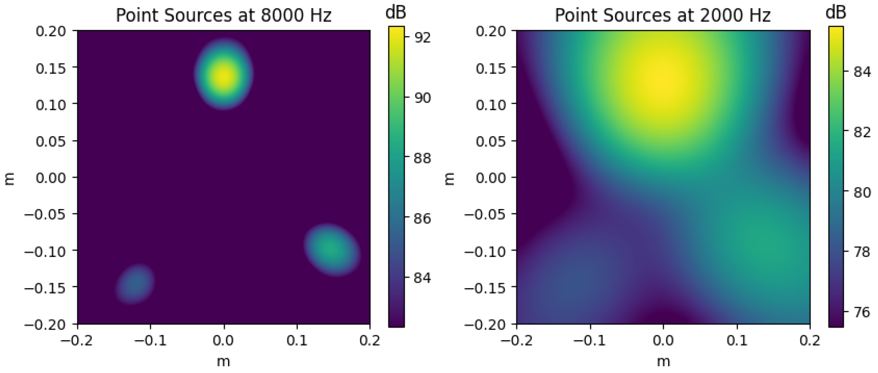
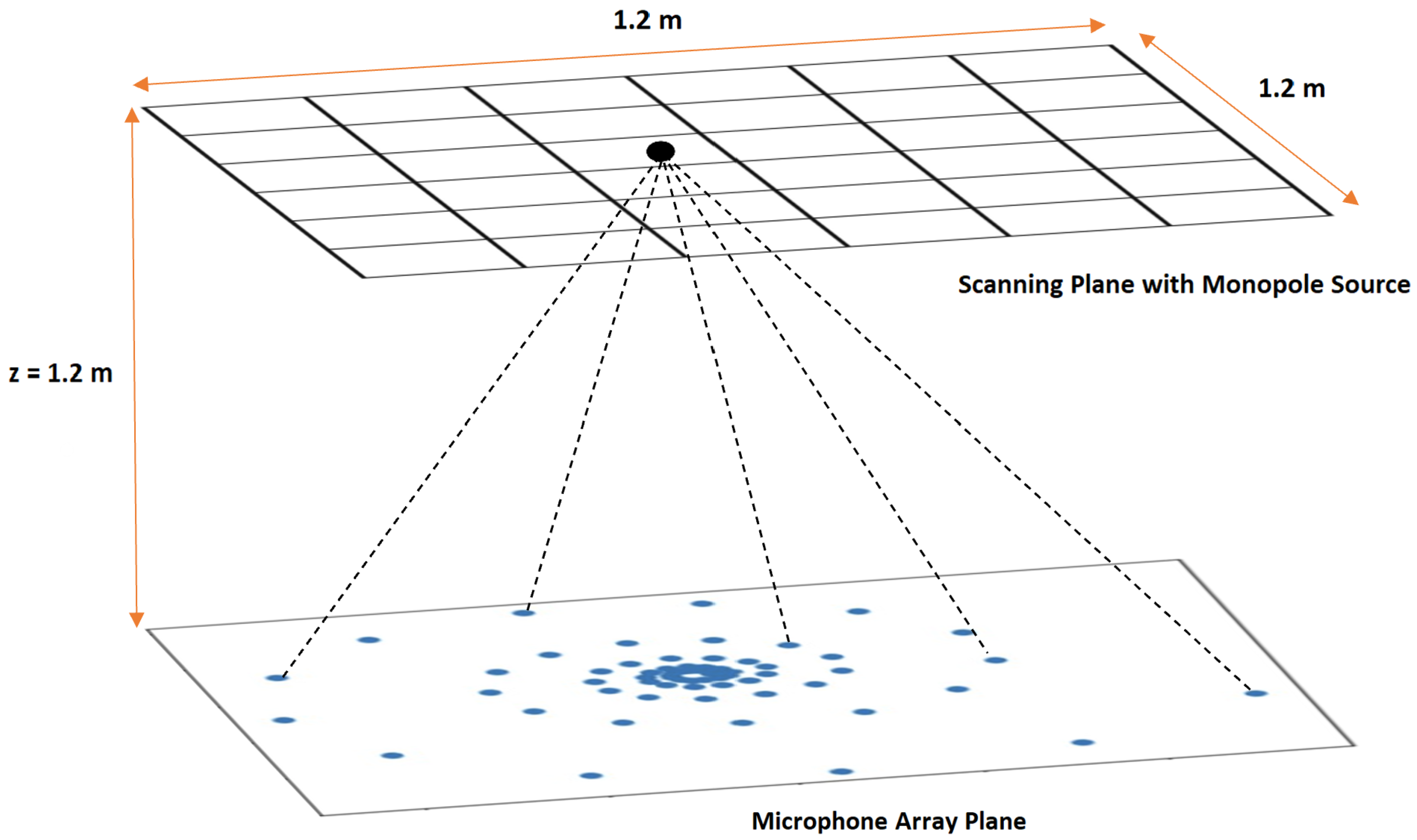
3.1. Case 1: Stationary Source Localization on a Scanning Plane

This case takes inspiration from the work by Xu et al. [18], Ma and Liu [27]. Xu et al. [18], in particular, carried out source localization on a scanning plane parallel to the microphone array plane for a wide frequency range of 200 to 20,000 Hz, using a deep neural network called DenseNet-201. They were able to show the superiority of DenseNet-201 over other classic acoustic imaging methods. However, DenseNet needed a significant amount of simulated data, memory, and processing power to train. In this paper, we focused on ASL at two frequencies in the low-frequency range (100 Hz and 300 Hz) using limited training data and a shallow CNN to prove that ASL is possible using a computationally less expensive approach. The setup is shown in Figure 7.

We used a scanning plane of dimensions 1.2 m × 1.2 m. The scanning plane was located $1.2$ m above the array plane containing the 64-microphone logarithmic spiral array, as described in the previous section. To generate the training dataset, S monopole sources (S1, Equation (1)) with unit source strength were randomly distributed throughout the $N\times N$ scanning grid. The acoustic pressure of all sources was calculated at all the microphones (M) to form the combined pressure vector, P, given as:

$$\begin{array}{c}\hfill P=\left[\sum _{s=1}^S{P}_s\left(1\right),\sum _{s=1}^S{P}_s\left(2\right),\sum _{s=1}^S{P}_s\left(3\right),\dots ,\sum _{s=1}^S{P}_s\left(M\right)\right]\end{array}$$

(3)

Vector P, in turn, was used to obtain the cross-spectral matrix (CSM) as:

$$\begin{array}{c}\hfill \mathrm{CSM}=P{P}^H\end{array}$$

(4)

where $P^H$ is the conjugate transpose of P. The dimensions of the CSM are $M\times M$, which in this case is $64\times 64$. The CSM represents the power distribution over frequency, and we used the real part of it as an input feature to the CNN. The CSM here serves a different purpose than what it traditionally serves in signal processing. In the context of deep learning, the CSM is an image-like input feature that encapsulates the acoustic pressure information needed to train our CNN. The CNN was trained against the ground truth, i.e., the source distribution from which the CSM was derived, to predict the strength and location of the sources. For the ground truth, the $N\times N$ scanning grid was converted to a $N^2\times 1$ binary vector in which the elements corresponding to the sources were assigned the value 1 (equal to the source strength), and the elements without a source were assigned the value 0. We defined the output layer as a dense layer with $N^2$ nodes without an activation function, thus treating this as a regression problem. We use the Rectified Linear Unit (ReLU) activation function everywhere throughout the network. The network prediction was a vector of output layer dimensions ($N^2\times 1$) that was compared against the ground truth vector to calculate the loss. The loss function used was the mean squared error (MSE), defined as:

$$\begin{array}{c}\hfill MSE={\displaystyle \frac{{\sum }_{i=1}^n{(y_{pred}-y_{gt})}^2}{n}}\end{array}$$

(5)

where, $y_{pred}$ is the predicted vector given by the network, $y_{gt}$ is the ground truth vector, and n is the length of the two vectors, which in this case is $N^2$. The optimizer used was ADAM [33] with the default values of the hyperparameters. Details of the CNN and the training process are given in Section 4.

3.2. Case 2: Two-Dimensional ASL on the Horizon

This case used a classification approach to determine the direction of arrival (DoA) of the acoustic signal from a source located on the horizon. The four-microphone array was used for this case and the azimuth angle ($\theta$) had to be determined. The range of possible values of $\theta$ (0–180°) was discretized into N classes. The output of the network is the probability distribution of all the classes, and the class with the highest probability is the estimated DoA. The setup is shown in Figure 8.

Since this case uses a classification approach, the final dense layer of the network had the softmax activation function, which normalized the output of the network to give the probability distribution over N classes. ReLU activation was used everywhere else. ADAM was used as the optimizer while the loss function was cross-entropy, which is the standard loss function for classification problems [34]. We used both types of sources in this case, the monopole and the sinusoidal plane wave signal, and they have been discussed separately.

3.2.1. Case 2 (i): Monopole (S1)

To generate the training set, a monopole with unit source strength was placed at a real, random value of $\theta$ (in the range of $\theta$) from the center of the four-microphone array and at a fixed radial distance r (=10 m). The cross-spectral matrix was calculated with the same procedure as in case 1 and its real part was used as an input to a CNN. The value of $\theta$ falls into a certain class and the index of this class was the ground truth against which the network was trained.

3.2.2. Case 2 (ii): Sinusoidal Plane Wave (S2)

A sinusoidal plane wave signal (Equation (2)) was generated from a random direction (real, random value of $\theta$) and fixed r (=10 m) from the origin. The signal was polluted with white Gaussian noise. The amplitude of the pressure signal and the white noise were equal and set to 10 Pa. We applied the generalized cross-correlation (GCC) algorithm to all microphone pairs to generate an input feature. GCC is a time delay of arrival (TDOA) approach and is known to be robust to noise and reverberation. The GCC vector between two signals $r_1\left(t\right)$ and $r_2\left(t\right)$ is defined as the inverse Fourier transform (IFFT) of the cross-power spectrum [35]:

$$\begin{array}{c}\hfill \mathrm{GCC}=\mathrm{IFFT}(R_1\odot R_2^{*})\end{array}$$

where, $R_1$ and $R_2$ are the STFT vectors for $r_1$ and $r_2$, ⊙ represents element-wise multiplication, and * represents the complex conjugate.

Figure 9 shows a sample GCC pattern obtained using a pair of microphone signals polluted with uncorrelated noise. It can be seen that, while the signals are distorted, the GCC pattern is still very evident. The entire GCC vector was not used as input. For each microphone pair, there are a certain number of correlation coefficients near the center that contain useful information. These coefficients were extracted from the GCC feature map to be used as input to the CNN. The calculation for the number of coefficients is as follows. The maximum possible time delay ($\tau$) between two microphones for the four-microphone array shown in Figure 5 is given by the distance between two microphones (2 m) and the speed of sound (343 m/s) as $\tau =2/343=5.83$ ms. For a sampling frequency of 16,000 Hz, the maximum delay in samples is n = 16,000$\tau \approx 93$. So it is only the first 93 coefficients from the center of the GCC that contain useful information for each microphone pair. The first 93 GCC coefficients from the GCC of all microphone pairs (6) were concatenated to form a vector of size ($558\times 1$) and then reshaped into a matrix of dimensions ($31\times 18$). This reshaped matrix was used as input to the CNN. Of course, the vector of GCC coefficients can be directly fed to a multi-layer perceptron (MLP); however, a CNN is generally more powerful and accurate for classification problems. The CNN also has fewer learnable parameters compared with MLP, which reduces the risk of overfitting.

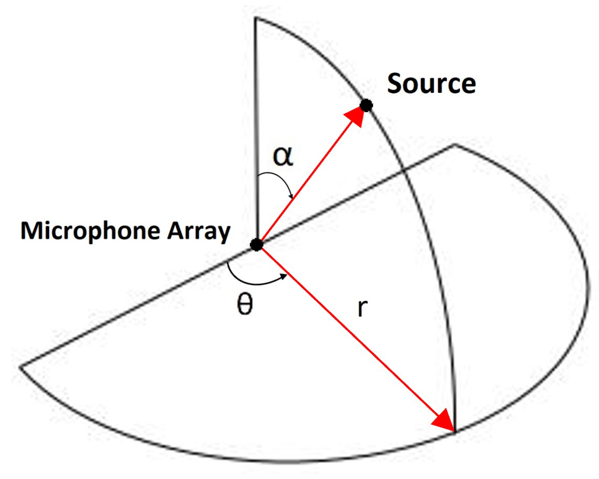
3.3. Case 3: Three-Dimensional ASL

This case is an extension of case 2. Similar to case 2, we used the four-microphone array and the two sources (cases 3 (i) for S1 and 3 (ii) for S2) with a classification approach for this case. The ranges of the azimuth angle, $\theta$, and the elevation angle, $\alpha$, were discretized into $N_1$ and $N_2$ classes, respectively. The setup is shown in Figure 10. We placed the source (S1 and S2 in separate sub-cases) at real, random values of $\theta$ and $\alpha$ and fixed r (=10 m) and used the real part of the resulting CSM to train the CNN. However, instead of using a conventional CNN, we used a multi-task CNN in which the separate tasks of determining $\theta$ and $\alpha$ were performed simultaneously by a single model. This is made possible because both tasks rely on the same input feature (CSM for S1 and GCC for S2). Separate networks for $\theta$ and $\alpha$ are an option (like case 2); however, it is not very efficient as individual datasets have to be generated and each network has to be trained separately. A multi-task network improves data efficiency and reduces training time and the chances of overfitting significantly as the model has to generalize over multiple tasks. Figure 11 shows the block diagram of the multi-task CNN used. This is an example of hard-parameter sharing, wherein the tasks share hidden layers while having task-specific output layers [36]. For both output branches ($\theta$ and $\alpha$), the activation function in the last layer was Softmax, and ReLU activation was used everywhere else. The optimizer and the loss function were ADAM and cross-entropy respectively, for both branches.

All CNN models in this paper were built using the deep learning frameworks Keras and Tensorflow, the details of which are shown in

Table 1. Summary of the convolutional neural network architecture used in all the cases.

Cases	Conv. Layers, Dimension	Max-Pool Layers, Dimension	Dense Layers (Nodes), Output Dimension
1	3, ($3\times 3$), Filters: 32, 64, 64	2, ($2\times 2$)	4 (128), Output: 144
2 (i): S1	2, ($2\times 2$), Filters: 128, 64	None	1 (128), Output: N
2 (ii): S2	3, ($2\times 2$), Filters: 128, 64, 64	2, ($2\times 2$)	1 (128), Output: N
3 (i): S1	2, ($2\times 2$), Filters: 128, 64	None	($\theta$): 1 (128), $N_1$ ($\alpha$): 1 (128), $N_2$
3 (ii): S2	2, ($2\times 2$), Filters: 128, 64, 64	2, ($2\times 2$)	($\theta$): 1 (128), $N_1$ ($\alpha$): 1 (128), $N_2$

. The training for all the cases was carried out on Google Colaboratory.

4. Results

Table 1 gives the details of the CNN models used in all three cases.

4.1. Case 1

For case 1, the model was trained to detect six monopole sources that were spread across a 12 × 12 scanning grid plane by randomly assigning coordinates. The results are presented and compared for source frequencies of 100 Hz and 300 Hz. Xu et al. [18], who also presented results for six monopole source localization using DenseNet, generated a batch of 512 training samples and 1000 validation samples for each epoch and ran the model for almost 3000 epochs. This means the training was carried out with more than 4.5 million samples. In contrast, our shallow CNN model trained for 600 epochs on 50,000 training samples. The training data are 0.00045% of the total number of possible samples $\left({\displaystyle \genfrac{}{}{0pt}{}{144}{6}}\right)$, which is in the order of ≈${10}^{10}$, thus exemplifying the limited nature of the data. The CNN also had a significantly smaller number of learnable parameters (≈1 million) compared with DenseNet (≈20 million).

The details of the CNN model are given in Table 1. The learning rate for the optimizer was fine-tuned to 0.0001. This case took approximately 100 min to train. The obtained results were post-processed to highlight the strongest sources (predicted source strengths of 0.3 and higher) and allow us to derive qualitative and quantitative trends. Figure 12 and Figure 13 show two source configurations as predicted by the model for monopole sources at 300 Hz. Figure 14 and Figure 15 show similar results for monopole sources at 100 Hz. The red dots represent the ground truth source configuration. These results are followed by

Table 2. Source detection statistics for 1000 test samples. The frequency-dependence of model performance is evident—the model was able to detect more sources when they were oscillating at a higher frequency (300 Hz).

Sources Detected	300 Hz	100 Hz
6	9	1
5	70	10
4	272	39
3	397	142
2	210	344
1	42	348
0	0	116
Total	1000	1000

, which gives the source detection statistics at the two source frequencies for 1000 test samples.

Discussion

As mentioned, Xu et al. [18] used a batch of 512 training and 1000 validation samples each epoch while running the model for around 3000 epochs, the total number of samples thus amounting to ≈4.5 million. We limited our training data and epochs to 50,000 samples (≈$1\%$ of Xu et al. [18]) and 600 epochs, respectively, and sought to maximize the performance of the model under these constraints. While Xu et al. [18]’s DNN naturally showed superior performance given the vast computational resources employed, we found that, at a relatively higher source frequency of 300 Hz (Figure 12 and Figure 13), our model was able to capture the source distribution reasonably well with a limited dataset. The model showed good resolution, less spreading, and was able to detect sparse sources. The limit of the model’s performance was identified as 100 Hz since the results at 100 Hz source frequency and below (Figure 14 and Figure 15) with the same amount of training were relatively poor. The model struggled to locate the sources when they were sparsely located (Figure 14) and tended to perform better when they were located in clusters. The increase in spreading is evident from Figure 15 but is still much less than beamforming, wherein the poor resolution renders the results unusable at low frequencies. To resolve low-frequency sources using beamforming, the size of the scanning plane and the distance between the sources would have to be much more than the size of the plane used in this case. The CNN was able to resolve low-frequency sources on the current plane, thus highlighting its superior resolution and detection capabilities. Table 2 reaffirms statistically the frequency-dependent performance of the model. For a source frequency of 300 Hz, the model was able to detect the majority of the sources (four or more) in 35.1% samples (351 out of 1000 samples), and at least half of the sources (three or more) in 74.8% samples (748 out of 1000 samples). At 100 Hz source frequency, the percentages drop to 5% for detecting the majority of the sources (50 out of 1000 samples) and 19.2% for detecting at least half of the sources (192 out of 1000 samples). To obtain better results at 100 Hz and lower frequencies, we have to go beyond the set network architecture and training limits and increase the number of layers/training data samples/epochs. The effectiveness of the shallow CNN in terms of giving promising results with very limited data compared with Xu et al. [18]’s DNN makes it an avenue worth exploring further.

4.2. Case 2

In cases 2 and 3, which are classification-type problems, the performance was measured in terms of the prediction accuracy of the correct class (and thus the DoA) given by the model. In this case, the model predicted the class of $\theta$. The training was carried out using 50,000 training samples and 200 epochs with a fine-tuned learning rate of 0.0001. Since the source can be placed at any real value of $\theta$ between $0^{°}$ and ${180}^{°}$, the training set of 50,000 samples is very limited as the total number of possible cases is infinite. The results for the two types of sources used in case 2 are given in

Table 3. Accuracy values are for a test set of 10,000 samples for the monopole source. The sharp decline in accuracy for $N=180$ is a limitation of small-sized input.

Classes (N)	Class Size	Accuracy ($\mathit{\theta }$, 100 Hz)	Accuracy ($\mathit{\theta }$, 300 Hz)
20	9°	≈91%	≈95%
30	6°	≈89%	≈92%
45	4°	≈81%	≈91%
60	3°	≈69%	≈87%
90	2°	≈52%	≈77%
180	1°	≈23%	≈57%

and

Table 4. Accuracy values for a test set of 10,000 samples for a sinusoidal plane wave source. The accuracy (for 100 Hz and 300 Hz) is higher and the drop-off in model performance as N increases is gradual as compared with the monopole source, thus highlighting the superiority of GCC as an input feature in this case.

Classes (N)	Class Size	Accuracy ($\mathit{\theta }$, 10 Hz)	Accuracy ($\mathit{\theta }$, 100 Hz)	Accuracy ($\mathit{\theta }$, 300 Hz)
20	9°	≈84%	≈97%	≈98%
30	6°	≈76%	≈96%	≈97%
45	4°	≈63%	≈95%	≈96%
60	3°	≈52%	≈93%	≈95%
90	2°	≈40%	≈89%	≈93%
180	1°	≈20%	≈79%	≈86%

.

4.2.1. Case 2 (i): Monopole (S1)

We used a monopole source at 100 Hz and 300 Hz to evaluate the model’s performance under the set training constraints. The source was at a radial distance of 10 m (r = 10 m) from the center of the four-microphone array. Since the dimensions of the cross-spectral matrix (CSM) were small ($4\times 4$ for the four-microphone array), only two convolutional layers, without pooling layers, were used in the CNN (Table 1). The variation in accuracy of $\theta$ with the number of classes N for both source frequencies is shown in Table 3.

4.2.2. Case 2 (i): Sinusoidal Plane Wave (S2)

For this source, the drop in model performance was not as drastic as the monopole, which allowed us to test for source frequencies well into the infrasound range. Results are provided for a sinusoidal plane wave source polluted with uncorrelated noise at 10 Hz (infrasound), 100 Hz, and 300 Hz. The distance of the source from the array was 10 m ($r=10$ m); however, the distance does not matter in this case as the amplitude does not undergo any decay and remains constant. The vector formed by concatenating the extracted portions from the GCC vectors of the microphone pairs ($558\times 1$) was reshaped into a matrix ($31\times 18$) and fed to the CNN. The larger size of the image allowed us to apply more convolution and pooling layers. Table 4 shows the prediction accuracy of the model and its dependence on the number of classes.

4.2.3. Discussion

For the monopole source, the prediction accuracy of the model for both source frequencies was very high when the number of classes was less (20), and decreased gradually as the number of classes increased. Between the two source frequencies, the model performed better at the higher frequency. The small size of the input image (CSM) significantly reduced the network size and the parameters to be optimized, hence the model trained very quickly. At the same time, a small input reduced the scope of learning as we were very limited in the number of convolution and pooling layers that we could apply. A consequence of this is the drop in performance as the problem becomes more complex. Fewer convolution layers means that the network cannot learn deeper and more abstract features of a complex problem, resulting in potentially overfitting and a decrease in the accuracy of prediction. This can be seen in Table 3. While the model can give good results in this case, when the number of classes N is small, the drop-off in performance is stark as N increases. This is a clear limitation of the CSM as an input feature with few microphones.

In the case of the sinusoidal plane wave source (Table 4), the GCC map allowed us to obtain an appropriately sized input feature. At the same time, selectively picking the portion of the GCC feature map containing the essential information helped keep the input size in check to save computational time and resources.

Comparing the accuracy values for source frequencies 100 Hz and 300 Hz in Table 4 with those obtained for the monopole source (Table 3), it is evident that the model displays a superior performance with the GCC input feature, which is again down to the difference in the input size. The model can thus learn much better with GCC as the input. This highlights the advantage of using a time-domain input feature (GCC) as opposed to a frequency-domain feature (CSM) for detecting very low source frequencies when the number of microphones is limited. For the infrasound source, the accuracy for smaller class sizes can be improved with more training. An accuracy value greater than 60% for 45 classes for an infrasound source in the presence of noise shows the robustness and reliability of GCC as an input feature.

4.3. Case 3

As this case is more challenging than case 2, the number of training samples was increased to 80,000, keeping the number of epochs at 200 and the learning rate at 0.0001. The learning rate was set to 0.0001. The resolution or class size was kept the same for $\theta$ and $\alpha$, resulting in different numbers of classes, $N_1$ and $N_2$, respectively. The performance of the model was measured in terms of the prediction accuracy of the correct class for $\theta$ and $\alpha$. For this case, we provide representative results at a single source frequency as the trends in the results will be similar to the results in case 2.

4.3.1. Case 3 (i): Monopole (S1)

Representative results are provided for a monopole source oscillating at 100 Hz. The real part of the CSM (dimensions $4\times 4$) was used as an input to the multi-task CNN. The prediction accuracy of the model is shown in

Table 5. Prediction accuracy for $\theta$ and $\alpha$ in three-dimensional ASL with a monopole source at 100 Hz for 10,000 samples. There is no negative transfer since the accuracy values for $\theta$ and $\alpha$ decrease at a similar rate.

Class Size	${\mathit{N}}_1$ ($\mathit{\theta }$)	Accuracy ($\mathit{\theta }$)	${\mathit{N}}_2$ ($\mathit{\alpha }$)	Accuracy ($\mathit{\alpha }$)
10°	18	≈93%	9	≈91%
5°	36	≈84%	18	≈79%
3°	60	≈69%	30	≈58%
2°	90	≈56%	45	≈52%
1°	180	≈29%	90	≈36%

.

4.3.2. Case 3 (ii): Sinusoidal Plane Wave (S2)

Representative results are provided for a sinusoidal plane wave source at 10 Hz. The GCC coefficient matrix of size $(31\times 18)$ (same as case 2 (ii)) was used as an input to the multi-task CNN. The prediction accuracy of the model is shown in

Table 6. Prediction accuracy for $\theta$ and $\alpha$ in three-dimensional ASL with a sinusoidal plane wave source at 10 Hz for 10,000 samples. Negative transfer is evident as the accuracy of $\theta$ prediction declines rapidly compared with $\alpha$.

Class Size	${\mathit{N}}_1$ ($\mathit{\theta }$)	Accuracy ($\mathit{\theta }$)	${\mathit{N}}_2$ ($\mathit{\alpha }$)	Accuracy ($\mathit{\alpha }$)
10°	18	≈79%	9	≈99%
5°	36	≈58%	18	≈99%
3°	60	≈41%	30	≈97%
2°	90	≈26%	45	≈96%
1°	180	≈13%	90	≈91%

.

4.3.3. Discussion

The multi-task CNN utilizes the same input feature for performing two related tasks—classifying the azimuth angle, $\theta$, and the elevation angle, $\alpha$. A commonly encountered problem in multi-task learning is “negative transfer”, wherein one or more tasks can dominate the training/learning process and hurt the performance of other tasks. The tasks whose performance is hampered tend to perform better in a single-task model compared with a multi-task model [37]. Both tasks are learned reasonably well in the case of a monopole source (Table 5) but a clear case of negative transfer is observed for the sinusoidal plane wave source (Table 6). The prediction of $\alpha$ dominates the training, which is expected as it is the easier of the two tasks ($N_2<N_1$). However, the prediction accuracy values for $\theta$ are less than what were obtained when a single-task model was used for predicting $\theta$ in case 2(ii). A suggested way to overcome negative transfer is to weigh the individual losses from the two tasks appropriately such that they are on the same scale [37].

5. Conclusions

We developed three benchmark cases for low- and very-low-frequency passive acoustic source localization using deep learning. The limitations of conventional beamforming necessitated the use of a deep learning-based approach. The cases used a shallow CNN with limited training data and sought to optimize the performance at low source frequencies under the training constraints. We obtained promising qualitative and quantitative results, and it can be concluded that the benchmark cases collectively prove the viability of deep learning-based approaches for low- and very-low-frequency ASL. At the same time, the results provide insight into the network and training parameters that can be changed to further expand the scope of these cases and obtain better results. The size of the input feature is also an aspect to be considered. Smaller input sizes would be reduced by the network to the point that learning from them would become very difficult as the problem becomes more and more complex. We would like to mention that, while obtaining good results with shallow networks and limited data is feasible, with the appropriate resources, deeper networks like ResNets and DenseNets can be trained to give better results; however, the dataset must be commensurate with the size of the network otherwise the network will tend to overfit the data and generalize poorly. Studies employing ResNet-50 used between 200–800 million training samples to prevent overfitting.

References

1. Peyvandi, H.; Farrokhrooz, M.; Roufarshbaf, H.; Park, S.J. SONAR systems and underwater signal processing: Classic and modern approaches. In SONAR Systems; IntechOpen: London, UK, 2011; pp. 173–206. [Google Scholar]
2. Carter, G. Time delay estimation for passive sonar signal processing. IEEE Trans. Acoust. Speech Signal Process. 1981, 29, 463–470. [Google Scholar] [CrossRef]
3. Fernandes, J.d.C.V.; de Moura Junior, N.N.; de Seixas, J.M. Deep learning models for passive sonar signal classification of military data. Remote Sens. 2022, 14, 2648. [Google Scholar] [CrossRef]
4. Tosi, P.; Sbarra, P.; De Rubeis, V. Earthquake sound perception. Geophys. Res. Lett. 2012, 39, L24301. [Google Scholar] [CrossRef]
5. Hill, D.P.; Fischer, F.G.; Lahr, K.M.; Coakley, J.M. Earthquake sounds generated by body-wave ground motion. Bull. Seismol. Soc. Am. 1976, 66, 1159–1172. [Google Scholar]
6. Sylvander, M.; Ponsolles, C.; Benahmed, S.; Fels, J.F. Seismoacoustic recordings of small earthquakes in the Pyrenees: Experimental results. Bull. Seismol. Soc. Am. 2007, 97, 294–304. [Google Scholar] [CrossRef]
7. Bocanegra, J.A.; Borelli, D.; Gaggero, T.; Rizzuto, E.; Schenone, C. A novel approach to port noise characterization using an acoustic camera. Sci. Total Environ. 2022, 808, 151903. [Google Scholar] [CrossRef]
8. Booth, E.; Humphreys, W. Tracking and characterization of aircraft wakes using acoustic and lidar measurements. In Proceedings of the 11th AIAA/CEAS Aeroacoustics Conference, Monterey, CA, USA, 23–25 May 2005; p. 2964. [Google Scholar]
9. Joshi, A.; Rahman, M.M.; Hickey, J.P. Recent Advances in Passive Acoustic Localization Methods via Aircraft and Wake Vortex Aeroacoustics. Fluids 2022, 7, 218. [Google Scholar] [CrossRef]
10. Schönhals, S.; Steen, M.; Hecker, P. Towards wake vortex safety and capacity increase: The integrated fusion approach and its demands on prediction models and detection sensors. Proc. Inst. Mech. Eng. Part G J. Aerosp. Eng. 2013, 227, 199–208. [Google Scholar] [CrossRef]
11. Shams, Q.A.; Zuckerwar, A.J.; Burkett, C.G.; Weistroffer, G.R.; Hugo, D.R. Experimental investigation into infrasonic emissions from atmospheric turbulence. J. Acoust. Soc. Am. 2013, 133, 1269–1280. [Google Scholar] [CrossRef]
12. Watson, L.M.; Iezzi, A.M.; Toney, L.; Maher, S.P.; Fee, D.; McKee, K.; Ortiz, H.D.; Matoza, R.S.; Gestrich, J.E.; Bishop, J.W.; et al. Volcano infrasound: Progress and future directions. Bull. Volcanol. 2022, 84, 44. [Google Scholar] [CrossRef]
13. Chiariotti, P.; Martarelli, M.; Castellini, P. Acoustic beamforming for noise source localization–Reviews, methodology and applications. Mech. Syst. Signal Process. 2019, 120, 422–448. [Google Scholar] [CrossRef]
14. de Santana, L. Fundamentals of Acoustic Beamforming; NATO Educ. Notes EN-AVT; NATO Science and Technology Organization: Brussels, Belgium, 2017; Volume 4. [Google Scholar]
15. Gombots, S.; Nowak, J.J.; Kaltenbacher, M. Sound source localization–state of the art and new inverse scheme. Elektrotech. Infor. e & i 2021, 138, 229–243. [Google Scholar]
16. Rayleigh, F.R.S. XXXI. Investigations in optics, with special reference to the spectroscope. Lond. Edinb. Dublin Philos. Mag. J. Sci. 1879, 8, 261–274. [Google Scholar] [CrossRef]
17. Brooks, T.F.; Humphreys, W.M. A deconvolution approach for the mapping of acoustic sources (DAMAS) determined from phased microphone arrays. J. Sound Vib. 2006, 294, 856–879. [Google Scholar] [CrossRef]
18. Xu, P.; Arcondoulis, E.J.; Liu, Y. Acoustic source imaging using densely connected convolutional networks. Mech. Syst. Signal Process. 2021, 151, 107370. [Google Scholar] [CrossRef]
19. Sarradj, E.; Herold, G. A Python framework for microphone array data processing. Appl. Acoust. 2017, 116, 50–58. [Google Scholar] [CrossRef]
20. Bianco, M.J.; Gerstoft, P.; Traer, J.; Ozanich, E.; Roch, M.A.; Gannot, S.; Deledalle, C.A. Machine learning in acoustics: Theory and applications. J. Acoust. Soc. Am. 2019, 146, 3590–3628. [Google Scholar] [CrossRef]
21. Grumiaux, P.A.; Kitić, S.; Girin, L.; Guérin, A. A survey of sound source localization with deep learning methods. J. Acoust. Soc. Am. 2022, 152, 107–151. [Google Scholar] [CrossRef]
22. Yalta, N.; Nakadai, K.; Ogata, T. Sound source localization using deep learning models. J. Robot. Mechatronics 2017, 29, 37–48. [Google Scholar] [CrossRef]
23. Vera-Diaz, J.M.; Pizarro, D.; Macias-Guarasa, J. Towards end-to-end acoustic localization using deep learning: From audio signals to source position coordinates. Sensors 2018, 18, 3418. [Google Scholar] [CrossRef]
24. O’Shea, K.; Nash, R. An introduction to convolutional neural networks. arXiv 2015, arXiv:1511.08458. [Google Scholar]
25. Chakrabarty, S.; Habets, E.A. Broadband DOA estimation using convolutional neural networks trained with noise signals. In Proceedings of the 2017 IEEE Workshop on Applications of Signal Processing to Audio and Acoustics (WASPAA), New Paltz, NY, USA, 15–18 October 2017; pp. 136–140. [Google Scholar]
26. Xiao, X.; Zhao, S.; Zhong, X.; Jones, D.L.; Chng, E.S.; Li, H. A learning-based approach to direction of arrival estimation in noisy and reverberant environments. In Proceedings of the 2015 IEEE International Conference on Acoustics, Speech and Signal Processing (ICASSP), South Brisbane, QLD, Australia, 19–24 April 2015; pp. 2814–2818. [Google Scholar]
27. Ma, W.; Liu, X. Phased microphone array for sound source localization with deep learning. Aerosp. Syst. 2019, 2, 71–81. [Google Scholar] [CrossRef]
28. Huang, G.; Liu, Z.; Van Der Maaten, L.; Weinberger, K.Q. Densely connected convolutional networks. In Proceedings of the IEEE Conference on Computer Vision and Pattern Recognition, Honolulu, HI, USA, 21–26 July 2017; pp. 4700–4708. [Google Scholar]
29. Niu, H.; Gong, Z.; Ozanich, E.; Gerstoft, P.; Wang, H.; Li, Z. Deep learning for ocean acoustic source localization using one sensor. arXiv 2019, arXiv:1903.12319. [Google Scholar]
30. He, K.; Zhang, X.; Ren, S.; Sun, J. Deep residual learning for image recognition. In Proceedings of the IEEE Conference on Computer Vision and Pattern Recognition, Las Vegas, NV, USA, 27–30 June 2016; pp. 770–778. [Google Scholar]
31. Prime, Z.; Doolan, C. A comparison of popular beamforming arrays. In Proceedings of the Australian Acoustical Society AAS2013 Victor Harbor, Victor Harbor, Australia, 17–20 November 2013; Volume 1, p. 5. [Google Scholar]
32. Albawi, S.; Mohammed, T.A.; Al-Zawi, S. Understanding of a convolutional neural network. In Proceedings of the 2017 International Conference on Engineering and Technology (ICET), Antalya, Turkey, 21–23 August 2017; pp. 1–6. [Google Scholar]
33. Kingma, D.P.; Ba, J. Adam: A method for stochastic optimization. arXiv 2014, arXiv:1412.6980. [Google Scholar]
34. Ho, Y.; Wookey, S. The real-world-weight cross-entropy loss function: Modeling the costs of mislabeling. IEEE Access 2019, 8, 4806–4813. [Google Scholar] [CrossRef]
35. Varzandeh, R.; Adiloğlu, K.; Doclo, S.; Hohmann, V. Exploiting periodicity features for joint detection and DOA estimation of speech sources using convolutional neural networks. In Proceedings of the ICASSP 2020—2020 IEEE International Conference on Acoustics, Speech and Signal Processing (ICASSP), Barcelona, Spain, 4–8 May 2020; pp. 566–570. [Google Scholar]
36. Amyar, A.; Modzelewski, R.; Li, H.; Ruan, S. Multi-task deep learning based CT imaging analysis for COVID-19 pneumonia: Classification and segmentation. Comput. Biol. Med. 2020, 126, 104037. [Google Scholar] [CrossRef]
37. Lakkapragada, A.; Sleiman, E.; Surabhi, S.; Wall, D.P. Mitigating negative transfer in multi-task learning with exponential moving average loss weighting strategies (student abstract). In Proceedings of the AAAI Conference on Artificial Intelligence, Washington, DC, USA, 7–14 February 2023; Volume 37, pp. 16246–16247. [Google Scholar]
Figure 1. Comparison of beamforming result for point sources (located at (0, 0.14, 0.3), (0.15, −0.1, 0.3), and (−0.12, −0.15, 0.3)) emitting white noise signals over 1/3 octave bands with center frequencies of 8000 Hz and 2000 Hz, obtained using the open-source beamforming framework developed by Sarradj and Herold [19].
Applsci 14 09893 g001
Figure 2. Flow of data in the method. This structure is followed by all the test cases developed in this paper.
Applsci 14 09893 g002
Figure 3. Summary of the test cases. All the cases use the framework shown in Figure 2.
Applsci 14 09893 g003
Figure 4. A 64-channel, simulated, logarithmic spiral-shaped microphone array.
Applsci 14 09893 g004
Figure 5. Four microphone array. All coordinates are in meters. The three outer microphones form an equilateral triangle while the fourth microphone is at the midpoint of the altitude.
Applsci 14 09893 g005
Figure 6. An example showing a convolutional neural network and the impact of convolution and pooling layers on the image size and information transfer.
Applsci 14 09893 g006
Figure 7. Case 1: Acoustic source localization on a scanning plane. The scanning plane is discretized into an N × N grid of uniform resolution. The finer the grid size is, the higher is the computational cost.
Applsci 14 09893 g007
Figure 8. Case 2: Two-dimensional ASL on the horizon. Two possible source configurations S 1 and S 2 are shown. θ < 90 ° for S 1 while θ > 90 ° for S 2 . r = 10 . The source coordinates for these two positions are ( r cos θ , r sin θ ) and ( r cos θ , r sin θ ) , respectively.
Applsci 14 09893 g008
Figure 9. GCC pattern for a pair of microphone signals polluted with uncorrelated noise. The GCC feature map is symmetric about the origin. Therefore the useful correlation coefficients can be picked from either side of the origin.
Applsci 14 09893 g009
Figure 10. Case 3: Three-dimensional ASL. The four-microphone is shown as a point. The localization domain is a quarter sphere ( 0 ° θ 180 ° , 0 ° α 90 ° , r = 10 ). The coordinates of the source are ( r sin ( α ) cos ( θ ) , r sin ( α ) sin ( θ ) , r cos ( α ) ) .
Applsci 14 09893 g010
Figure 11. A multi-task CNN used for three-dimensional ASL. The main branch performed the convolution and pooling operations on the input feature. The two output branches peeled off the main branch using the flattened feature vector as the input to give separate predictions for θ and α .
Applsci 14 09893 g011
Figure 12. Source configuration 1 (300 Hz). These are representative results at this source frequency. The legend is in Pascals (Pa), representing source strength.
Applsci 14 09893 g012
Figure 13. Source configuration 2 (300 Hz).
Applsci 14 09893 g013
Figure 14. Sparse sources (100 Hz). The model struggles at lower frequencies when the concentration of sources is less.
Applsci 14 09893 g014
Figure 15. Clustered sources (100 Hz). The model performs relatively better when low-frequency sources are highly concentrated.
Applsci 14 09893 g015