Comparison Between InterCriteria and Correlation Analyses over sEMG Data from Arm Movements in the Horizontal Plane

Abstract

InterCriteria analysis (ICrA) and two kinds of correlation analyses, Pearson (PCA) and Spearman (SCA), were applied to surface electromyography (sEMG) signals obtained from human arm movements in the horizontal plane. Ten healthy participants performed ten movements, eight of which were cyclic. Each cyclic movement (CM) consisted of flexion and extension phases with equal duration (10 s, 6 s, 2 s, and 1 s) and two 5 s rest poses between them. The CMs were performed with and without an added load of 0.5 kg on the wrists of the participants. The sEMG signals from six different muscles or separate muscle heads (m. deltoideus pars clavicularis, m. deltoideus pars spinata, m. brachialis, m. anconeus, m. biceps brachii, and m. triceps brachii long head) were recorded and used to compare the results of the ICrA, PCA, and SCA. All three methods found identical consonance pairs for the flexion and extension CM phases. Additionally, PCA detected two more consonance pairs in the extension phases. In this investigation, ICrA, PCA, and SCA were proven to be reliable tools when applied separately or in combination for sEMG data. These three methods are appropriate for researching arm movements in the horizontal plane and experimental protocol revision.

1. Introduction

Decision making in healthcare and biomedicine is a complex and hard-to-solve task. The process is associated with different restrictions and often requires multiple compromises. Recently developed by Atanassov et al., InterCriteria analysis (ICrA) [1] has been proven in different papers as a promising tool for estimating biological data that support successful decision-making processes. Until now, this approach has been used for solving real-world tasks such as in medicine [2,3,4], kinesiology [5,6], and sports [7], as well as in ecology [8,9], economics [10,11], artificial intelligence [12,13,14], etc. The novelty of the ICrA in comparison to other well-established methods like Pearson’s and Spearman’s correlation analyses is mentioned in Traneva and Tranev, 2021, and Atanassov et al., 2014 [1,15]. ICrA is based only on “<, >, =” comparisons between object scores against the investigated criteria instead of their numerical values. Thus, the calculations involved become faster than those with other methods for correlation analysis (CA). ICrA can be applied to both clear data and incomplete and fuzzy data. ICrA evaluates the degree of correspondence, not correspondence, and the degree of “uncertainty” between the criteria.

Applying only one approach is sometimes not enough to solve a particular problem. This is why several papers use CA along with ICrA. For example, Todinova et al. [16] use ICrA and Pearson’s CA (PCA) to define the relations between calorimetric and statistical parameters derived from blood plasma proteome thermograms of patients with colorectal cancer. In this research, both approaches are distinguished as helpful tools for in-depth analyses of calorimetric data sets. Also, Todinova et al. show that ICrA and PCA complement each other. In eight cases, ICrA exceeds the PCA, and for the other eight, PCA surpasses the ICrA. Krumova et al. [17] test the same decision-making methods along with Spearman’s CA (SCA) for calorimetric and biochemical parameters obtained from the serum proteome of patients suffering from multiple myeloma (MM). In this work, the authors report strong similarities between results from ICrA and SCA that help to determine the interrelations between calorimetric and biochemical data for MM. Vassilev et al. [18] verify two new ICrA modifications using real data from prostate carcinoma patients. The outcomes from the two modifications of the ICrA, classical ICrA, and the widely used PCA are similar. The methods find closeness between the same criteria, with almost analogous values. Antonov [7] also aims to establish the correlations and directions of dependencies between model indicators of the basic and specialized speeds of twenty young hockey players by applying ICrA and PCA. The author reports that PCA, traditionally used in sports science, gives correlations and dependencies confirmed or rejected by ICrA.

ICrA was used for the first time over surface electromyography (sEMG) signals in [5,6]. Electromyography (EMG) is a widely used technique for detecting and analyzing biological signals [19]. Two types of electrodes can be used—needle (invasive) and surface electrodes (noninvasive). EMG measures muscle responses from an action potential generated in the central nervous system. It is transmitted electrochemically through the nerve fibers and stimulates multiple skeletal muscle fibers [19]. EMG in dynamic conditions gives information on muscle intensity and velocity, which reveal the forces exerted over the human joints [20,21]. Once acquired, EMG helps to understand the behavior of the human body under normal and pathological conditions. This knowledge is most applicable in sports science and rehabilitation and for diagnosing different neuro-muscular diseases, estimating the forces developed by the muscles, and controlling prosthetic devices [22,23]. Part of recovery medicine includes robots, exoskeletons, orthosis, etc., where EMG signals are used for intention prediction for movement and its realization [24]. In addition, the interaction between sEMG and fluid-driven innovations opens fields for control that enable the realization of complex and more motion-precise robotic systems with adaptable structures [25,26]. In the analysis of EMG signals, various computational methods are used, depending on the aim, such as variance analysis, Fisher’s least square differences posthoc test [27], principal component analysis, and convolutional neural network [28], InterCriteria analysis [5,6], and correlation analysis [29,30,31], as well as different computational methods for data augmentation [32].

SCA and PCA are widely applied in upper arm EMG research. Aoyama and Kohno, 2020, studied the hand dexterity motor skills among thirty-eight neurologically healthy participants by assessing the temporal and quantitative variabilities in their muscle activity [33]. They apply Spearman’s rank CA to find the relationship between the time of task performance (ball rotation) and the coefficient of variation of the EMG on-phase duration. The next correlation is searching between the ball rotation time and coefficient of variation of the EMG on-phase area over thirty trials for all participants. Other authors uses Spearman’s rank correlation to assess the paretic muscles of thirty-two patients in the chronic stroke stage [29]. They evaluate the relationship between the Fugl-Meyer assessment scores for the upper arm and the percentage of the facilitation of forearm EMG activity. Another work examined arm chronic plegia in twenty-four patients [30]. Spearman’s rank correlation and Mann–Whitney’s U-test are used for the following assessed quantities: upper extremity and spinal cord motor and functional independence, capabilities of the upper extremity, muscle strength of the elbow flexors and extensors, and EMG of right m. biceps brachii and m. triceps brachii.

Some studies use Pearson’s correlation method during EMG examinations. Nougeria-Neto et al. [27] investigate the muscle fatigue of m. biceps brachii during submaximal isometric contractions, using EMG and mechanomyography. Ten healthy men perform the required tasks for the elbow. Different statistical analyses over four signal segments for each contraction are applied. Also, Pearson’s CA is applied over similar physiological events to search for strong correlations. Other authors use Pearson’s CA to investigate the signal-to-noise ratio in EMG signals that are artificially contaminated [31]. Their results show that lower Pearson’s correlation coefficients are associated with low signal-to-noise values.

Conducting biomedical research to obtain EMG signals poses several challenges to investigators. Some scientists aim to study healthy individuals, while others focus on people with specific movement disorders. Knowledge of normal human kinetics can help to understand the pathological processes occurring due to trauma and injury. The main task of biomedical research is to create a sufficiently broad and informative protocol that does not burden the subject. It should involve motor tasks that are easy to perform, repeatable, and accessible with the abilities of research subjects who have different motor cultures. However, a detailed explanation and several practice movements are required before the real experimental trial to ensure the movements are right. In our experimental protocol, along with the specific movements, there is another difficulty—participants should perform tasks with a specific duration. This requires more attention, concentration, and training. Increased attention leads to mental fatigue. This means that shortening the time for the entire examination will preserve the participant’s condition. In addition to mental fatigue, a long duration of exercise causes muscle fatigue to build up. Fatigue changes the biomechanical characteristics of the muscle. These, in turn, change the interpretation of results, which is critical for biomedical studies. In addition, fatigue also reflects the participant’s condition. Sometimes, prolonged motor activity and maintaining poses can lead to inconvenience, discomfort, or even pain. Emotions (confusion, embarrassment, feelings of stress, etc.) can also be affected [34]. These sensations are more pronounced in disordered people due to their diseases. A basic principle in conducting research with people is their humane treatment.

The human factor also includes the interests of the researchers who perform such experiments. The principle of fatigue during an experiment also concerns them. Post-processing of the data would be easier if a higher percentage of these data had useful EMG signals, without artifacts and the need to apply additional filtration. All this is reflected in the time invested.

From the point of view of the equipment used, especially the electrodes, the prolonged electrode–skin connection could loosen. From here, the signal quality and the recorded useful signal decrease as an analysis quantity. For a deep study, a large number of useful signals are needed. This presupposes the availability of human resources and a solid database. This, in turn, means investing a large amount of finances and human resources. For example, the European Union spent 8.4 billion in 2023 on health research [35].

Therefore, a well-planned protocol, tight during its execution, with few losses of useful signals and preserved informativeness, is essential for conducting biomedical research.

Neither ICrA nor correlation analyses have been used in horizontal arm movement investigations until now. The purpose of the paper is applying ICrA, PCA, and SCA for detecting the correlations between the active phases of elbow flexion and extension during horizontal plane movements in the presence of two variables—speed and weight. The obtained outcomes will be compared and, in addition, a suggestion for the revision of the experimental protocol will be provided.

2. Materials and Methods

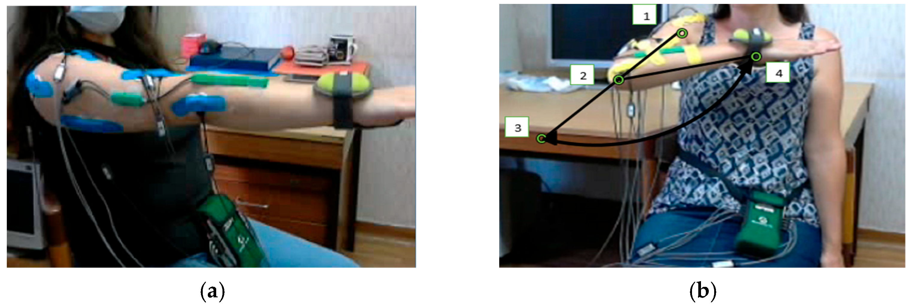
2.1. Experimental Protocol

An experimental study was conducted with fifteen volunteers. The data of only four women and six men were retained for consideration here. Although the smaller sample size complicates summarizing the findings, may not properly represent the target group, and limits the generalizability for a larger set of volunteers, the other five participants were excluded from further consideration. The reasons for exclusion were various - the existence of numerous artifacts in the raw sEMG signal, the inability to perform the movement in the required tact, and inaccurate positioning of the limbs. Commonly, sEMG artifacts can be caused by the following factors: improper electrode placement, power line interference, cross-talk, noise originating from devices in the surrounding area, physiological artifacts coming from the heartbeat, breathing movements, sweating, static electricity charge, electrodes, cables, and skin movement. To reduce all these possible artifact appearances, we strictly stuck to the Seniam protocol for skin preparation and electrode placement [36]; used the battery mode of computer operation to avoid 50 Hz contamination; recorded big, easy to find surface muscles to avoid cross-talk; switched off any electrical devices, as well as not using an internet connection; investigated the right arm muscles so no heart rate was registered; avoided synthetic materials; and used Butterworth filters to reduce artifacts of the shaking of the skin, subcutaneous tissue, and muscles.

All the participants were in a good general condition and had no related musculoskeletal or neuronal complaints. The subjects were thoroughly informed about the upcoming procedure and provided their informed consent. They were then asked to complete a series of eighteen motor tasks (MTs)–calm position, evoking maximal isometric contractions, eight cyclic movements (CMs) in the sagittal plane, and eight CMs in the horizontal plane. The Scientific Council of the Institute of Biophysics and Biomedical Engineering approved the investigation.

Until now, two articles have been published detailing the first part of the motion protocol performed in the sagittal plane [5,6]. This article focuses on movements performed in the horizontal plane.

The sEMG signals were registered by the circle electrodes “Skintact-premier” F-301 Ag/AgCl and the Telemyo 2400G2 system of Noraxon Inc. (Scottsdale, AZ, USA). As the SENIAM protocol recommends [36], the electrodes were placed over precisely defined areas of the previously chosen surface muscles. The skin underwent preparation aiming for better contact with the electrode and obtaining a good output signal. If necessary, the skin area was shaved and treated with alcohol. Electrode gel was then applied, and the electrodes were placed over the following muscles: m. deltoideus pars clavicularis (DELcla), m. deltoideus pars spinata (DELspi), m. brachialis (BRA), m. anconeus (ANC), m. biceps brachii (BIC), and m. triceps brachii long head (TRI). The angle at the elbow joint was also measured with a 2D goniometer, again produced by Noraxon Inc. The goniometer was calibrated for each person before the start of the experimental series.

The experimental series was explained and demonstrated to the participants in detail. Before the start of each recording, the participant performed as many repetitions of the movement as necessary to complete the required time interval of one minute, which was conducted with video and sEMG data recordings.

Here, we will discuss only the MTs performed in the horizontal plane and the tasks used further for sEMG signal normalization.

Each participant sat on a stable chair without armrests. The spine was kept straight, and their gaze was directed forward. The arms were freely relaxed next to the body, and the feet were firmly placed on the floor. All MTs were performed with the dominant arm of the person—the right one.

• MT 1: Calm position. The subject was sitting on a chair. He took the position described above and kept it for one minute. This record aimed to follow the reliability of all the signals of the six muscles and the angle.
• MT 2: Evoking of maximal isometric contractions. The examiner passively moved the subject’s upper limb into six different starting positions. A contraction began in the musculature from these positions. The subject opposed the examiner’s controlled resistance, applied in the distal part of the bones. As a result, there was a maximum rise in muscle tension without allowing movement in the joints. Thus, instead of isotonic, the muscle contraction became isometric.

A set of identical movements followed. To prepare for them, the participant brought their right arm straight forward (90° shoulder flexion) before the one-minute recording began. The palm was facing down, as shown in Figure 1. From this position, four alternating phases were performed in sequence.

-

The first phase was elbow flexion—flexion was limited to the point when the thumb touched the opposite shoulder.

-

The second phase was a posture, i.e., the final flexed position was retained.

-

The third phase was elbow extension—the arm moved from the flexed position until the arm was extended straight ahead.

-

The fourth phase was again a pose—the final extended position was held.

All flexion and extension phases were equal and continued for 10 s, 6 s, 2 s, or 1 s. The poses were held for 5 s.

An ergonomic weight was placed on the wrist of the hand (Figure 1b). The experimental protocol continued with the sequence of motor tasks 3, 4, 5, and 6. The difference was in the additional weight added in motor tasks 7, 8, 9, and 10.

• MT 3: Flexions and extensions in the horizontal plane—active phases lasting 10 s, denoted in the paper as fH10 and eH10.
• MT 4: Flexions and extensions in the horizontal plane—active phases lasting 6 s, denoted here as fH6 and eH6.
• MT 5: Flexions and extensions in the horizontal plane—active phases lasting 2 s, denoted here as fH2 and eH2.
• MT 6: Flexions and extensions in the horizontal plane—active phases lasting 1 s, denoted here as fH1 and eH1.
• MT LOAD 7: Flexions and extensions in the horizontal plane with the attached weight. The active phases lasted 10 s (denoted in this paper as eH10w and eH10w).
• MT LOAD 8: Flexions and extensions in the horizontal plane with the attached weight. The active phases lasted 6 s (eH6w and eH6w).
• MT LOAD 9: Flexions and extensions in the horizontal plane with the attached weight. The active phases lasted 2 s (eH2w and eH2w).
• MT LOAD 10: Flexions and extensions in the horizontal plane with the attached weight. The active phases lasted 1 s (eH1w and eH1w).

Each experimental trial was stored in a separate text file, which contained information on time, the sEMGs of the six muscles, and the elbow flexion/extension angle.

Filtration was used for MT 1 and MT 2 (Butterworth high-pass filter, 4th order, cut-off frequency of 20 Hz; Butterworth low-pass filter, 4th order, cut-off frequency of 250 Hz) [37]. The filtered data were inspected for artifacts. For MT 2, the signal was further rectified, and time intervals without artifacts were chosen. For these intervals, the maximal EMG values were calculated. They were used for the normalization coefficients.

For motor tasks 3, 4, 5, 6, 7, 8, 9, and 10, filtration (Butterworth high-pass filter, 4th order, cut-off frequency of 20 Hz; Butterworth low-pass filter, 4th order, cut-off frequency of 250 Hz) was used, and the data were normalized to the calculated coefficients. These four intervals for each movement were rectified and smoothed (20 samples). The area under the obtained curves was calculated and divided into the respective time intervals. The obtained values were further analyzed by ICrA, PCA, and SCA.

2.2. ICrA Analysis

InterCriteria analysis combines index matrices (IMs) and intuitionistic fuzzy sets (IFS) for establishing the dependencies (positive or negative consonance) along with the dissonances between the considered criteria [1]. For the initial ICrA application, it is necessary to prepare data sets of multiple objects measured against different criteria, presented in the form of an index matrix (IM) as follows:

	Obj1	…	Objk	…	Objn
Cr1	eCr1,Obj1	…	eCr1,Objk	…	eCr1,Objn
…	…	…	…	…	…
Cri	eCri,Obj1	…	eCri,Objk	…	eCri,Objn
…	…	…	…	…	…
Crm	eCrm,Obj1	…	eCrm,Objk	…	eCrm,Objn

In the initial IM Cr₁ … Cr_m denotes criteria; Obj₁ … Obj_n represents objects; and e_Cr1,Obj1 … e_Crm,Objn are elements, respectively. IM elements are commensurated by relation R, so that for each i, j, k is defined R(e_Crk, _Obji, e_Crk, _Objj).

Let $N_{k,l}^{\mu }$ and $N_{k,l}^{\upsilon }$ be the numbers of cases in which R(e_Crk, _Obji, e_Crk, _Objj) and R(e_Crl, _Obji, e_Crl, _Objj) and, respectively, R(e_Crk, _Obji, e_Crk, _Objj) and $\overline{R}$(e_Crl, _Obji, e_Crl, _Objj) are simultaneously satisfied. $\overline{R}$ is the dual relation of $R$, so if $R$ is satisfied, $\overline{R}$ is not satisfied, and vice versa.

Then, we obtain the following:

$$N_{k,l}^{\mu }+N_{k,l}^{\upsilon } \le {\displaystyle \frac{n(n-1)}{2}}$$

(1)

From Equation (1), we obtain two numbers for each k, l, (1 ≤ k < l ≤ m) and for n ≥ 2 as follows:

$${\mu }_{Crk,Crl}=2{\displaystyle \frac{N_{k,l}^{\mu }}{n(n-1)}}, {\upsilon }_{Crk,Crl}=2{\displaystyle \frac{N_{k,l}^{\upsilon }}{n(n-1)}}$$

(2)

where ${\mu }_{Crk,Crl}, {\upsilon }_{Crk,Crl}$ is an intuitionistic fuzzy pair (IFP) that presents intuitionistically fuzzy evaluations of the relations established between Cr_k and Cr_l.

Thus, the final IM, which contains the relationships between the criteria, is obtained in the following form:

	Cr1	…	Cri	…	Crm
Cr1	〈1, 0〉	…	${\mu }_{Cr1,Cri},{\upsilon }_{Cr1,Cri}$	…	${\mu }_{Cr1,Crm},{\upsilon }_{Cr1,Crm}$
…	…	…	…	…	…
Cri	${\mu }_{Cri,Cr1},{\upsilon }_{Cri,Cr1}$	…	〈1, 0〉	…	${\mu }_{Cri,Crm},{\upsilon }_{Cri,Crm}$
…	…	…	…	…	…
Crm	${\mu }_{Crm,Cr1},{\upsilon }_{Crm,Cr1}$	…	${\mu }_{Crm,Cri},{\upsilon }_{Crm,Cri}$	…	〈1, 0〉

The final IM sets the degrees of correspondence and non-correspondence between the criteria Cr₁, …, Cr_m. Also, the degree of uncertainty is calculated. ICrA correlation dependencies have intuitionistic fuzzy pairs form with values between 0 and 1. The algorithm determines the degrees of correlation between the criteria, known as positive or negative consonance and dissonance, depending on the threshold values α and β (0 ≤ α ≤ 1, 0 ≤ β ≤ 1, and α + β ≤ 1) for μ and ν. The two criteria Cr_k and Cr_l are in positive consonance (PC) when ${\mu }_{Crk,Crl}$ > α and ${\upsilon }_{Crk,Crl}$ < β, or the µ value is in the interval (0.75, 1.00]. Negative consonance (NC) is detected when ${\mu }_{Crk,Crl}$ < β and ${\upsilon }_{Crk,Crl}$ > α, or the µ value is in the interval [0.00, 0.25]. Dissonance appears in the other cases, when the µ value is in the interval (0.25, 0.75]. According to [38,39], the threshold values are α = 0.75 and β = 0.25.

In greater detail, according to [1,38], PC can be considered as strong (µ ∈ (0.95, 1.00]), only positive (µ ∈ (0.85, 0.95]), and weak (µ ∈ (0.75, 0.85]). The same is valid for NC and dissonance. There is strong (µ ∈ (0.15, 0.25]), only negative (µ ∈ (0.05, 0.15]) and weak (µ ∈ [0.00, 0.05]) NC, as well as strong (µ ∈ (0.43, 0.57]), only dissonance (µ ∈ (0.57, 0.67] and µ ∈ (0.33, 0.43]), and weak (µ ∈ (0.67, 0.75] and µ ∈ (0.25, 0.33]) dissonance.

For all ICrA calculations in the paper, ICrAData software, version 2.5, is used with the most common µ-biased algorithm, where α = 0.75 and β = 0.25 by default [39]. The ICrAData software is freely available at: http://intercriteria.net/software/ (accessed on 29 May 2024)

2.3. Correlation Analyses of Pearson and Spearman

Correlation analysis quantitatively describes the strength of correlational dependencies through statistical indicators called correlation coefficients that carry this information [40]. Correlation coefficients can take values between −1 and 1. The absolute value of the coefficient provides information for the strength of the dependence between two variables, X and Y, and also, the sign of the correlation coefficient provides information for the direction of dependences. A positive number indicates positive relations between the variables, i.e., if one variable increases, the other is expected to also increase. A negative coefficient indicates negative relations between the variables. If one variable increases, the other is expected to decrease.

The value of the correlation coefficient (r) determines the strength of the correlation. According to [41], when r = 0, there is no correlation. When r = 1, there is a perfect (so-called functional) correlation. When the absolute value of the correlation coefficient r is between the following:

• 0.00 and 0.09, there is a negligible correlation;
• 0.10 and 0.39, there is a weak correlation;
• 0.40 and 0.69, there is a significant correlation;
• 0.70 and 0.89, there is a strong correlation;
• 0.90 and 1.00, there is a very strong correlation.

Pearson’s simple linear correlation coefficient is calculated by the following formula:

$$r={\displaystyle \frac{P}{SxSy}}$$

(3)

where P is the moment of the products. Sx is the deviation of the variable X. Sy is the corresponding standard deviation of the variable Y. P is calculated by the following formula:

$$P={\displaystyle \frac{\sum XY}{n-1}}-{\displaystyle \frac{\sum X\sum Y}{n(n-1)}}$$

(4)

where ∑X is the sum of the values of X, ∑Y is the sum of the values of Y, ∑XY is the sum of the X and Y products, and n is the sample size.

Spearman’s rank correlation coefficient is calculated using the following formula:

$$r_s=1-{\displaystyle \frac{6\sum d^2}{n(n^2-1)}}$$

(5)

where d is the difference in the rank numbers of X and Y and n is the sample size.

The two CAs were implemented over the sEMG data using the capabilities provided by Microsoft Excel (v. 2023).

3. Results

Surface EMG signals from the six muscles or muscle heads, obtained from ten healthy subjects, are used in this paper to compare the results of ICrA, PCA, and SCA. The sEMG data for participants one and ten (P1 and P10) are presented in Figure 2. The sEMG data for the rest of the volunteers will not be shown here to avoid the repetition of similar figures.

The sEMG data for Delcla, Delspi, BIC, TRI, ANC, and BRA for the flexion and extension phases with different durations with or without an added load were processed by ICrA, PCA, and SPA. Two IMs consisting of the criteria and objects were created for each participant (from P1 to P10). Eight flexion or extension phases were the criteria. The calculated areas under the obtained curves of the EMG signals for the six muscles or muscle heads were the objects. The results in the form of heat maps for twenty-eight flexion or extension phases’ pairs after ICrA application are given in

Table 1. Results obtained by ICrA for eight flexion phases for all participants.

Flexion	P1	P2	P3	P4	P5	P6	P7	P8	P9	P10
fH10–fH6	0.93	0.47	1.00	1.00	1.00	1.00	0.93	1.00	0.87	0.80
fH10–fH2	0.93	0.40	0.73	0.93	0.93	0.93	0.93	0.93	0.47	0.67
fH10–fH1	0.93	0.33	0.67	0.93	1.00	0.93	0.87	0.93	0.80	0.80
fH10–fH10w	0.93	0.27	0.73	1.00	0.93	0.93	0.87	1.00	0.83	0.67
fH10–fH6w	0.93	0.33	0.73	0.87	1.00	1.00	0.87	0.93	0.53	0.60
fH10–fH2w	0.93	0.40	0.73	0.87	1.00	0.93	0.87	0.93	0.80	0.67
fH10–fH1w	0.87	0.40	0.60	0.80	1.00	0.93	0.87	0.93	0.93	0.80
fH6–fH2	1.00	0.93	0.73	0.93	0.93	0.93	0.87	0.93	0.60	0.87
fH6–fH1	1.00	0.87	0.67	0.93	1.00	0.93	0.80	0.93	0.93	0.87
fH6–fH10w	1.00	0.80	0.73	1.00	0.93	0.93	0.80	1.00	0.67	0.60
fH6–fH6w	1.00	0.87	0.73	0.87	1.00	1.00	0.80	0.93	0.67	0.53
fH6–fH2w	1.00	0.80	0.73	0.87	1.00	0.93	0.80	0.93	0.93	0.60
fH6–fH1w	0.93	0.67	0.60	0.80	1.00	0.93	0.80	0.93	0.93	0.73
fH2–fH1	1.00	0.93	0.80	1.00	0.93	1.00	0.93	1.00	0.53	0.87
fH2–fH10w	1.00	0.87	1.00	0.93	0.87	0.87	0.93	0.93	0.93	0.60
fH2–fH6w	1.00	0.80	1.00	0.93	0.93	0.93	0.93	1.00	0.93	0.67
fH2–fH2w	1.00	0.87	1.00	0.80	0.93	1.00	0.93	1.00	0.67	0.60
fH2–fH1w	0.93	0.73	0.87	0.87	0.93	1.00	0.93	1.00	0.53	0.73
fH1–fH10w	1.00	0.93	0.80	0.93	0.93	0.87	1.00	0.93	0.60	0.73
fH1–fH6w	1.00	0.87	0.80	0.93	1.00	0.93	0.87	1.00	0.60	0.67
fH1–fH2w	1.00	0.93	0.80	0.80	1.00	1.00	0.87	1.00	0.87	0.73
fH1–fH1w	0.93	0.80	0.93	0.87	1.00	1.00	1.00	1.00	0.87	0.87
fH10w–fH6w	1.00	0.93	1.00	0.87	0.93	0.93	0.87	0.93	0.87	0.93
fH10w–fH2w	1.00	0.87	1.00	0.87	0.93	0.87	0.87	0.93	0.60	1.00
fH10w–fH1w	0.93	0.73	0.87	0.80	0.93	0.87	1.00	0.93	0.60	0.87
fH6w–fH2w	1.00	0.80	1.00	0.87	1.00	0.93	1.00	1.00	0.73	0.93
fH6w–fH1w	0.93	0.67	0.87	0.93	1.00	0.93	0.87	1.00	0.60	0.80
fH2w–fH1w	0.93	0.87	0.87	0.80	1.00	1.00	0.87	1.00	0.87	0.87
	strong positive consonance							strong dissonance
	positive consonance							dissonance
	weak positive consonance							weak dissonance
	pair in positive consonance

and

Table 2. Results obtained by ICrA for eight extension phases for all participants.

Extension	P1	P2	P3	P4	P5	P6	P7	P8	P9	P10
eH10–eH6	1.00	0.87	1.00	1.00	0.93	1.00	0.93	0.93	0.87	1.00
eH10–eH2	0.93	0.87	0.73	1.00	1.00	1.00	1.00	0.93	0.60	0.87
eH10–eH1	0.93	0.47	0.73	1.00	1.00	1.00	0.87	0.93	0.80	0.93
eH10–eH10w	0.80	0.73	0.73	1.00	0.93	1.00	0.87	1.00	1.00	0.80
eH10–eH6w	1.00	0.80	0.73	0.93	0.93	1.00	0.87	0.93	0.60	0.73
eH10–eH2w	1.00	0.67	0.73	1.00	0.93	0.93	1.00	0.87	0.93	0.87
eH10–eH1w	0.93	0.60	0.73	0.87	0.87	1.00	0.93	0.93	0.93	0.93
eH6–eH2	0.93	0.87	0.73	1.00	0.93	1.00	0.93	1.00	0.60	0.87
eH6–eH1	0.93	0.60	0.73	1.00	0.93	1.00	0.93	1.00	0.80	0.93
eH6–eH10w	0.80	0.87	0.73	1.00	0.87	1.00	0.93	0.93	0.87	0.80
eH6–eH6w	1.00	0.80	0.73	0.93	0.87	1.00	0.93	0.87	0.73	0.73
eH6–eH2w	1.00	0.80	0.73	1.00	0.87	0.93	0.93	0.93	0.93	0.87
eH6–eH1w	0.93	0.73	0.73	0.87	0.80	1.00	0.87	1.00	0.93	0.93
eH2–eH1	1.00	0.60	1.00	1.00	1.00	1.00	0.87	1.00	0.67	0.93
eH2–eH10w	0.73	0.73	1.00	1.00	0.93	1.00	0.87	0.93	0.60	0.67
eH2–eH6w	0.93	0.80	1.00	0.93	0.93	1.00	0.87	0.87	0.73	0.60
eH2–eH2w	0.93	0.80	1.00	1.00	0.93	0.93	1.00	0.93	0.67	0.87
eH2–eH1w	0.87	0.73	1.00	0.87	0.87	1.00	0.93	1.00	0.67	0.93
eH1–eH10w	0.73	0.73	1.00	1.00	0.93	1.00	0.87	0.93	0.80	0.73
eH1–eH6w	0.93	0.67	1.00	0.93	0.93	1.00	0.87	0.87	0.67	0.67
eH1–eH2w	0.93	0.80	1.00	1.00	0.93	0.93	0.87	0.93	0.87	0.93
eH1–eH1w	0.87	0.87	1.00	0.87	0.87	1.00	0.80	1.00	0.87	1.00
eH10w–eH6w	0.80	0.93	1.00	0.93	0.87	1.00	1.00	0.93	0.60	0.93
eH10w–eH2w	0.80	0.93	1.00	1.00	0.87	0.93	0.87	0.87	0.93	0.67
eH10w–eH1w	0.73	0.87	1.00	0.87	0.93	1.00	0.80	0.93	0.93	0.73
eH6w–eH2w	1.00	0.87	1.00	0.93	1.00	0.93	0.87	0.80	0.67	0.73
eH6w–eH1w	0.93	0.80	1.00	0.80	0.93	1.00	0.80	0.87	0.67	0.67
eH2w–eH1w	0.93	0.93	1.00	0.87	0.93	0.93	0.93	0.93	1.00	0.93
	strong positive consonance							strong dissonance
	positive consonance							dissonance
	weak positive consonance							weak dissonance
	pair in positive consonance

. The purple colors, from light to dark, denote weak, only positive, and strong positive consonance. The grey colors, from light to dark, are used for weak, only dissonance, and strong dissonance.

According to the results presented in Table 1, a positive consonance (weak, only positive, and strong) was observed for six participants (P1, P4, P5, P6, P7, and P8) for all their twenty-eight flexion phases’ pairs. For the remaining four participants (P2, P3, P9, and P10), ICrA detected dissonances for some of the criteria pairs. The results given in Table 2 show the extension phases’ pairs only in positive consonance (weak, only positive, and strong) for five participants (P4, P5, P6, P7, and P8). Dissonance for some of the criteria pairs was found for the same number of investigated subjects (P1, P2, P3, P9, and P10).

Concerning the eight flexion/extension phases, ICrA found positive consonance between three criteria pairs for the same cyclic movements, namely fH1–fH1w, fH10w–fH6w, and fH2w–fH1w and eH1–eH2w, eH1–eH1w, and eH2w–eH1w. For the first two pairs of flexion and extension, weak, only positive, and strong positive consonance were observed, while for the third pair, only positive and strong positive consonances were detected. The interesting exception here is the pair eH10–eH6, which hit only positive and strong positive consonances for extension movements.

In this article, a positive consonance indicates the existing trends (increasing or decreasing) found in the muscle activity behavior that determine the correlated phase pairs. The dissonance was interpreted with no trends in muscle activity for the phases.

Pearson’s and Spearman’s CAs were also applied for the same data matrices.

The results for twenty-eight flexions and the same number of extension phases’ pairs after using the “CORREL” function for PCA calculations are presented as heat maps in

Table 3. Results obtained by PCA for eight flexion phases for all participants.

Flexion	P1	P2	P3	P4	P5	P6	P7	P8	P9	P10
fH10–fH6	1.00	0.43	0.81	0.98	1.00	1.00	0.99	0.97	0.96	0.74
fH10–fH2	0.99	0.27	0.36	0.99	0.98	0.96	1.00	0.84	−0.07	0.70
fH10–fH1	0.99	−0.02	0.39	0.99	0.99	0.90	0.99	0.66	0.68	0.90
fH10–fH10w	0.99	0.42	0.44	0.95	0.94	0.99	0.98	0.93	0.43	0.36
fH10–fH6w	0.98	0.28	0.44	0.93	0.96	0.90	0.98	0.93	0.60	0.00
fH10–fH2w	0.98	−0.21	0.44	0.78	0.99	0.87	0.99	0.56	0.94	0.42
fH10–fH1w	0.92	−0.16	0.38	0.91	0.99	0.86	0.98	0.66	0.94	0.67
fH6–fH2	1.00	0.97	−0.22	0.99	0.99	0.97	1.00	0.91	−0.08	0.90
fH6–fH1	0.99	0.77	−0.18	0.99	0.99	0.92	0.98	0.77	0.83	0.68
fH6–fH10w	0.99	0.97	−0.16	0.97	0.90	0.99	0.99	0.98	0.41	0.21
fH6–fH6w	0.98	0.96	−0.15	0.95	0.93	0.92	0.99	0.93	0.67	−0.07
fH6–fH2w	0.99	0.59	−0.15	0.81	0.97	0.89	1.00	0.67	0.99	0.38
fH6–fH1w	0.92	0.56	−0.20	0.92	0.97	0.89	0.97	0.78	0.93	0.51
fH2–fH1	0.99	0.88	0.96	0.97	0.98	0.98	0.99	0.96	−0.38	0.76
fH2–fH10w	1.00	0.91	0.97	0.98	0.93	0.98	1.00	0.98	0.87	−0.02
fH2–fH6w	1.00	0.94	1.00	0.98	0.93	0.98	0.99	0.99	0.66	−0.17
fH2–fH2w	1.00	0.69	0.97	0.88	0.97	0.96	1.00	0.91	−0.18	0.21
fH2–fH1w	0.95	0.68	0.96	0.95	0.97	0.95	0.98	0.96	−0.27	0.46
fH1–fH10w	0.98	0.75	0.96	0.95	0.88	0.95	0.98	0.88	0.20	0.43
fH1–fH6w	0.98	0.81	0.96	0.94	0.93	0.99	0.97	0.94	0.40	0.25
fH1–fH2w	0.99	0.92	0.97	0.80	0.97	0.99	0.98	0.99	0.86	0.58
fH1–fH1w	0.93	0.90	1.00	0.95	0.97	0.98	1.00	1.00	0.77	0.84
fH10w–fH6w	1.00	0.99	0.98	0.98	0.96	0.96	1.00	0.98	0.90	0.88
fH10w–fH2w	0.99	0.66	1.00	0.92	0.97	0.93	1.00	0.81	0.30	0.96
fH10w–fH1w	0.96	0.60	0.98	0.94	0.94	0.94	0.98	0.89	0.24	0.83
fH6w–fH2w	1.00	0.73	0.98	0.93	0.99	1.00	1.00	0.88	0.60	0.88
fH6w–fH1w	0.98	0.66	0.96	0.97	0.99	1.00	0.96	0.95	0.43	0.72
fH2w–fH1w	0.96	0.96	0.98	0.86	0.99	1.00	0.97	0.98	0.92	0.93
	perfect correlation							significant correlation
	very strong correlation							weak correlation
	strong correlation							negligible correlation
	pair in strong correlation							no correlation

and

Table 4. Results obtained by PCA for eight extension phases for all participants.

Extension	P1	P2	P3	P4	P5	P6	P7	P8	P9	P10
eH10–eH6	0.99	0.95	0.99	1.00	0.97	0.98	0.99	0.99	0.97	0.97
eH10–eH2	0.85	0.95	0.17	0.98	0.98	0.98	1.00	0.94	0.16	0.92
eH10–eH1	0.77	0.17	0.12	0.99	0.98	0.96	0.98	0.88	0.86	0.92
eH10–eH10w	1.00	0.89	0.17	0.98	0.98	0.99	0.98	0.95	1.00	0.82
eH10–eH6w	1.00	0.78	0.18	0.96	0.99	0.99	0.99	0.90	0.88	0.84
eH10–eH2w	0.81	0.63	0.19	0.89	0.99	0.93	1.00	0.80	0.95	0.85
eH10–eH1w	0.65	0.34	0.23	0.94	0.96	0.99	1.00	0.90	0.94	0.90
eH6–eH2	0.87	0.97	0.08	0.98	0.99	1.00	0.99	0.97	0.19	0.99
eH6–eH1	0.81	0.39	0.04	0.99	0.99	0.99	1.00	0.93	0.94	0.99
eH6–eH10w	0.98	0.97	0.07	0.99	0.92	0.99	1.00	0.94	0.98	0.73
eH6–eH6w	0.99	0.90	0.09	0.97	0.95	0.99	1.00	0.86	0.93	0.74
eH6–eH2w	0.82	0.82	0.01	0.89	0.94	0.97	0.99	0.87	0.99	0.82
eH6–eH1w	0.67	0.60	0.14	0.95	0.90	0.99	0.99	0.95	0.99	0.83
eH2–eH1	0.99	0.35	0.98	0.94	1.00	1.00	0.98	0.98	0.26	1.00
eH2–eH10w	0.80	0.93	0.96	0.97	0.94	0.98	0.98	0.84	0.11	0.66
eH2–eH6w	0.84	0.85	0.97	0.98	0.97	0.98	0.99	0.73	0.54	0.66
eH2–eH2w	0.99	0.75	0.95	0.96	0.95	0.95	1.00	0.90	0.20	0.79
eH2–eH1w	0.94	0.54	0.98	0.89	0.94	0.99	1.00	0.98	0.21	0.77
eH1–eH10w	0.72	0.51	0.99	0.98	0.96	0.97	0.99	0.79	0.87	0.69
eH1–eH6w	0.76	0.61	0.99	0.93	0.96	0.97	0.99	0.65	0.92	0.70
eH1–eH2w	0.98	0.77	0.98	0.83	0.95	0.96	0.99	0.95	0.98	0.83
eH1–eH1w	0.96	0.87	0.99	0.95	0.94	0.98	0.98	0.99	0.98	0.81
eH10w–eH6w	1.00	0.98	1.00	0.98	0.95	1.00	1.00	0.97	0.86	0.99
eH10w–eH2w	0.77	0.91	1.00	0.90	0.97	0.97	0.99	0.81	0.95	0.91
eH10w–eH1w	0.59	0.72	0.97	0.95	0.98	1.00	0.98	0.84	0.95	0.94
eH6w–eH2w	0.81	0.95	1.00	0.96	0.99	0.97	0.99	0.65	0.93	0.93
eH6w–eH1w	0.65	0.79	0.98	0.90	0.96	1.00	0.99	0.71	0.93	0.97
eH2w–eH1w	0.97	0.94	0.97	0.77	0.98	0.96	1.00	0.96	1.00	0.98
	perfect correlation							significant correlation
	very strong correlation							weak correlation
	strong correlation							negligible correlation
	pair in strong correlation							no correlation

. The purple colors from dark to light show perfect, very strong, and strong correlations. The gray colors from dark to light denote significant, weak, negligible, and no correlations, respectively.

As can be seen from Table 3 and Table 4, the PCA found strong, very strong, and perfect dependencies for five participants (P1, P4, P5, P6, and P7) when flexion is discussed, and for four participants (P4, P5, P6, and P7) when extension is in focus. Some values showed a smaller than strong dependence for the other five (P2, P3, P8, P9, and P10) and six participants (P1, P2, P3, P8, P9, and P10) for the flexion and extension phases. There were some flexion criteria pairs with negative dependences according to the PCA. These pairs were as follows: fH10–fH1, fH10–fH2w, and fH10–fH1w for P2; fH10–fH2, fH6–fH2, fH2–fH1, fH2–fH2w, and fH2–fH1w for P9; and fH6–fH6w, fH2–fH10w, and fH2–fH6w for P10. The PCA found three flexion phases’ pairs (fH1–fH1w, fH10w–fH6w, and fH2w–fH1w) and six extension phases’ pairs (eH10–eH6 eH1–eH2w, eH1–eH1w, eH10w–eH6w, eH10w–eH2w, and eH2w–eH1w) with strong, very strong, and perfect correlations.

Next, Spearman’s rank CA was applied to obtain the correlation values between the observed criteria. The data were ranked, and after that, the “CORREL” function embedded in Excel was used. The SCA results for the twenty-eight flexion and twenty-eight extension phases’ pairs are summarized as heat maps in

Table 5. Results obtained by SCA for eight flexion phases for all participants.

Flexion	P1	P2	P3	P4	P5	P6	P7	P8	P9	P10
fH10–fH6	0.94	−0.20	1.00	1.00	1.00	1.00	0.94	1.00	0.83	0.77
fH10–fH2	0.94	−0.26	0.43	0.94	0.94	0.94	0.94	0.94	−0.09	0.43
fH10–fH1	0.94	−0.37	0.31	0.94	1.00	0.94	0.83	0.94	0.77	0.77
fH10–fH10w	0.94	−0.43	0.43	1.00	0.94	0.94	0.83	1.00	−0.03	0.31
fH10–fH6w	0.94	−0.37	0.43	0.89	1.00	1.00	0.89	0.94	0.20	0.09
fH10–fH2w	0.94	−0.31	0.43	0.83	1.00	0.94	0.89	0.94	0.77	0.31
fH10–fH1w	0.89	−0.31	0.09	0.71	1.00	0.94	0.83	0.94	0.94	0.66
fH6–fH2	1.00	0.94	0.43	0.94	0.94	0.94	0.83	0.94	0.09	0.83
fH6–fH1	1.00	0.83	0.31	0.94	1.00	0.94	0.66	0.94	0.94	0.89
fH6–fH10w	1.00	0.77	0.43	1.00	0.94	0.94	0.66	1.00	0.14	0.31
fH6–fH6w	1.00	0.83	0.43	0.89	1.00	1.00	0.77	0.94	0.37	0.20
fH6–fH2w	1.00	0.66	0.43	0.83	1.00	0.94	0.77	0.94	0.94	0.31
fH6–fH1w	0.94	0.37	0.09	0.71	1.00	0.94	0.66	0.94	0.94	0.54
fH2–fH1	1.00	0.94	0.77	1.00	0.94	1.00	0.94	1.00	0.03	0.89
fH2–fH10w	1.00	0.83	1.00	0.94	0.89	0.89	0.94	0.94	0.94	0.43
fH2–fH6w	1.00	0.77	1.00	0.94	0.94	0.94	0.94	1.00	0.94	0.49
fH2–fH2w	1.00	0.83	1.00	0.71	0.94	1.00	0.94	1.00	0.14	0.43
fH2–fH1w	0.94	0.60	0.83	0.83	0.94	1.00	0.94	1.00	−0.03	0.60
fH1–fH10w	1.00	0.94	0.77	0.94	0.94	0.89	1.00	0.94	0.09	0.54
fH1–fH6w	1.00	0.83	0.77	0.94	1.00	0.94	0.89	1.00	0.26	0.49
fH1–fH2w	1.00	0.94	0.77	0.71	1.00	1.00	0.89	1.00	0.89	0.54
fH1–fH1w	0.94	0.71	0.94	0.83	1.00	1.00	1.00	1.00	0.89	0.83
fH10w–fH6w	1.00	0.94	1.00	0.89	0.94	0.94	0.89	0.94	0.89	0.94
fH10w–fH2w	1.00	0.89	1.00	0.83	0.94	0.89	0.89	0.94	0.09	1.00
fH10w–fH1w	0.94	0.60	0.83	0.71	0.94	0.89	1.00	0.94	0.09	0.83
fH6w–fH2w	1.00	0.71	1.00	0.83	1.00	0.94	1.00	1.00	0.43	0.94
fH6w–fH1w	0.94	0.37	0.83	0.94	1.00	0.94	0.89	1.00	0.26	0.77
fH2w–fH1w	0.94	0.89	0.83	0.77	1.00	1.00	0.89	1.00	0.83	0.83
	perfect correlation							significant correlation
	very strong correlation							weak correlation
	strong correlation							negligible correlation
	pair in strong correlation

and

Table 6. Results obtained by SCA for eight extension phases for all participants.

Extension	P1	P2	P3	P4	P5	P6	P7	P8	P9	P10
eH10–eH6	1.00	0.83	1.00	1.00	0.94	1.00	0.94	0.94	0.89	1.00
eH10–eH2	0.94	0.83	0.43	1.00	1.00	1.00	1.00	0.94	0.09	0.89
eH10–eH1	0.94	−0.14	0.43	1.00	1.00	1.00	0.89	0.94	0.77	0.94
eH10–eH10w	0.77	0.60	0.43	1.00	0.94	1.00	0.89	1.00	1.00	0.77
eH10–eH6w	1.00	0.71	0.43	0.94	0.94	1.00	0.89	0.94	0.43	0.66
eH10–eH2w	1.00	0.49	0.43	1.00	0.94	0.94	1.00	0.83	0.94	0.83
eH10–eH1w	0.94	0.26	0.43	0.83	0.89	1.00	0.94	0.94	0.94	0.94
eH6–eH2	0.94	0.89	0.43	1.00	0.94	1.00	0.94	1.00	0.09	0.89
eH6–eH1	0.94	0.31	0.43	1.00	0.94	1.00	0.94	1.00	0.66	0.94
eH6–eH10w	0.77	0.83	0.43	1.00	0.89	1.00	0.94	0.94	0.89	0.77
eH6–eH6w	1.00	0.77	0.43	0.94	0.83	1.00	0.94	0.83	0.60	0.66
eH6–eH2w	1.00	0.77	0.43	1.00	0.83	0.94	0.94	0.94	0.94	0.83
eH6–eH1w	0.94	0.66	0.43	0.83	0.77	1.00	0.89	1.00	0.94	0.94
eH2–eH1	1.00	0.31	1.00	1.00	1.00	1.00	0.89	1.00	0.31	0.94
eH2–eH10w	0.60	0.71	1.00	1.00	0.94	1.00	0.89	0.94	0.09	0.49
eH2–eH6w	0.94	0.77	1.00	0.94	0.94	1.00	0.89	0.83	0.66	0.37
eH2–eH2w	0.94	0.77	1.00	1.00	0.94	0.94	1.00	0.94	0.14	0.83
eH2–eH1w	0.89	0.60	1.00	0.83	0.89	1.00	0.94	1.00	0.14	0.94
eH1–eH10w	0.60	0.60	1.00	1.00	0.94	1.00	0.89	0.94	0.77	0.66
eH1–eH6w	0.94	0.43	1.00	0.94	0.94	1.00	0.89	0.83	0.49	0.60
eH1–eH2w	0.94	0.77	1.00	1.00	0.94	0.94	0.89	0.94	0.83	0.94
eH1–eH1w	0.89	0.83	1.00	0.83	0.89	1.00	0.77	1.00	0.83	1.00
eH10w–eH6w	0.77	0.94	1.00	0.94	0.89	1.00	1.00	0.94	0.43	0.94
eH10w–eH2w	0.77	0.94	1.00	1.00	0.89	0.94	0.89	0.83	0.94	0.60
eH10w–eH1w	0.60	0.89	1.00	0.83	0.94	1.00	0.77	0.94	0.94	0.66
eH6w–eH2w	1.00	0.89	1.00	0.94	1.00	0.94	0.89	0.77	0.49	0.66
eH6w–eH1w	0.94	0.77	1.00	0.66	0.94	1.00	0.77	0.83	0.49	0.60
eH2w–eH1w	0.94	0.94	1.00	0.83	0.94	0.94	0.94	0.94	1.00	0.94
	perfect correlation							significant correlation
	very strong correlation							weak correlation
	strong correlation							negligible correlation
	pair in strong correlation

, where perfect, very strong, and strong correlations are marked as dark, rose, and light purple, while the grayscale from dark to light denotes significant, weak, and negligible correlations.

It is obvious from Table 5 and Table 6 that, during flexion and extension movements for six (P1, P4, P5, P6, P7, and P8) and four participants (P5, P6, P7, and P8), there were only significant correlations for the twenty-eight phases’ pairs. Different correlations with low values were detected during flexion for four participants (P2, P3, P9, and P10) and during extension for six participants (P1, P2, P3, P4, P9, and P10). SCA detected some pairs of criteria with negative signs of the value for flexion phases. These pairs were fH10–fH6, fH10–fH2, fH10–fH1, fH10–fH10w, fH10–fH6w, fH10–fH2w, and fH10–fH1w for P2 and fH10–fH2, and fH2–fH1w for P9. Also, for P2, there was one pair, namely eH10–eH1, with negative dependence concerning extension. SCA found strong, very strong, and perfect correlations for the pairs fH1–fH1w, fH10w–fH6w, and fH2w–fH1w and eH10–eH6, eH1–eH2w, eH1–eH1w, and eH2w–eH1w.

4. Discussion

First, here, we will focus on the pairs of criteria in consonance dependence according to the three applied analyses in this investigation. The criteria pairs in consonance detected by ICrA, PCA, and SCA for the phases of flexion and extension are summarized in

Table 7. Detected by ICrA, PCA, and SCA criteria pairs in consonance.

ICrA		Pearson’s CA		Spearman’s CA
Flexion	Extension	Flexion	Extension	Flexion	Extension
fH1–fH1w fH10w–fH6w fH2w–fH1w	eH10–eH6 eH1–eH2w eH1–eH1w eH2w–eH1w	fH1–fH1w fH10w–fH6w fH2w–fH1w	eH10–eH6 eH1–eH2w eH1–eH1w eH10w–eH6w eH10w–eH2w eH2w–eH1w	fH1–fH1w fH10w–fH6w fH2w–fH1w	eH10–eH6 eH1–eH2w eH1–eH1w eH2w–eH1w

.

As can be seen from Table 7, ICrA and SCA found the same correlation pairs for flexion and extension phases. The PCA results were identical to those of ICrA and SCA when considering flexion pairs. PCA found two additional pairs in significant correlation for extension phases (eH10w–eH6w and eH10w–eH2w). Most relations in positive consonance were found for the phases of extension. Probably, this phase needs more muscle interactions to be performed precisely. It is hypothesized that the greater number of interactions during extension is a result of the neuromuscular mechanisms that increase joint stiffness to achieve better stabilization and kinetic control [42,43].

As expected, the three methods found a correlation between the flexion phases performed for 1 s with and without added weight (fH1–fH1w). The other two dependencies found by all three methods were only between flexion phases with different execution durations, in which a weight was placed. As can be seen from Table 7, the correlation pairs were between flexion phases with very close duration, 10 s and 6 s (fH10w–fH6w) and 2 s and 1 s (fH2w–fH1w).

Also, all three methods detected four identical correlation dependencies between extension phases. Three of them followed the logic described above. The correlation pairs were eH10–eH6, eH1–eH1w, and eH2w–eH1w. An unexpected correlation was found for the pair eH1–eH2w (weight existence). Furthermore, PCA detected one more unexpected correlation pair, namely eH10w–eH2w (too different velocities). These exceptions can be explained, since it is known that these approaches can find known as well as unknown relations.

All detected pairs in consonance for the flexion and extension phases were between relatively fast (fH2, eH2; fH2w, eH2w; fH1, eH1; and fH1w, eH1w) or relatively slow (fH10, eH10; fH10w, eH10w; fH6, eH6; and fH6w, eH6w) performed phases. There was only one exception, eH10w–eH2w, discovered for the extension phases by Pearson’s CA. It seems that the added weight of 0.5 kg did not influence the investigated correlations very much.

Based on the found correlations for the flexion and extension phases from the same cyclic MT, the researcher can omit some tasks from the experimental protocol. For the participants, it is more sparing to perform easier movements rather than harder movements, or shorter instead of longer ones [6,44]. Following the previously discussed specifics of the movements in the experimental protocol (EP), two kinds of optimized EP and the full EP are presented in

Table 8. Full and two kinds of optimized experimental protocols.

Full EP	Runtime [min]	I Optimized EP	Runtime [min]	II Optimized EP	Runtime [min]
MT 1	1	MT 1	1	MT 1	1
MT 2	1	MT 2	1	MT 2	1
MT 3	1	MT 3	1	MT 3	1
MT 4	1	MT 4	1	MT 4	1
MT 5	1	MT 5	1	MT 5	1
MT 6	1	MT 6	1	-	-
MT LOAD 7	1	MT LOAD 7	1	MT LOAD 7	1
MT LOAD 8	1	MT LOAD 8	1	MT LOAD 8	1
MT LOAD 9	1	MT LOAD 9	1	-	-
MT LOAD 10	1	-	-	MT LOAD 10	1
Total runtime, [min]	10	Total runtime, [min]	9	Total runtime, [min]	8

.

The first optimized EP is obtained after several decisions considering the results obtained from the three decision-making methods. When focusing on fH1–fH1w and eH1–eH1w, we can easily see that the consonance pairs include flexion and extension phases with equal durations, but one phase is performed with an added load. Hence, it is logical for fH1w and eH1w, respectively, as harder-to-perform tasks, to be excluded from the EP. These phases are parts of the MT LOAD 10 that will be omitted from the EP. Thus, the decision of which movement phase to remain from fH2w–fH1w and eH2w–eH1w becomes easier. In our case, fH2w and eH2w, as parts of MT LOAD 9, will be saved in the EP, while fH1w and eH1w will be removed.

If the analyses started from the consonance pairs fH2w–fH1w and eH2w–eH1w, it is obvious that the researcher must choose between the slower phase and the faster one, but with an added load. Since Park et al. [44] showed that, for participants, it is difficult to perform smooth rhythmic movements very slowly, fH1w could be preferred instead of fH2w. Hence, fH2w and eH2w from MT LOAD9 will be omitted. Also, from the pairs fH1–fH1w and eH1–eH1w, fH1 and eH1, as parts of MT 6, will be omitted to obtain a second optimized EP.

As shown in Table 8, the first version of the shortened EP takes one minute less than the time of the full EP, while the second optimized EP takes two minutes less. Hence, the procedure can save between 10% and 20% of the full EP execution time, but the saved time is more because the explaining and training time is not included here.

The outcomes of ICrA, PCA, and SCA were compared for each participant to examine the performances of the three approaches from another point of view. The identical results obtained by ICrA, PCA, and SCA for the twenty-eight flexion and twenty-eight extension phases are summarized in Figure 3.

The similarities in the results obtained by ICrA, PCA, and SCA for 56 correlation pairs (28 for flexion and 28 for extension) for each participant are discussed further. As can be seen from Figure 3, all mentioned methods calculated similar results (consonance or dissonance, respectively) for a major part of the correlation pairs. The most similarities (28 from possible 28) were found for P1, P4, P5, and P6, when flexion is in focus, while for extension, these participants were P5, P6, and P7. The least similarities between the results of the three algorithms were found for P2 and P8 (only 24) and P3 (only 16) for flexion and extension, respectively.

When the differences in the results of the three algorithms are discussed, the ICrA and SCA outcomes matched 34 correlation pairs (12 for flexion and 22 for extension). The matching results for PCA and SCA were found for sixteen correlation pairs, while for ICrA and PCA, they were only five. Again, it can be concluded that ICrA and SCA are more similar in evaluating results in comparison to ICrA and PCA, and PCA and SCA.

These theoretical results can be applied most successfully in rehabilitation and sports practice, where the degree of muscle loading is of great importance in the recovery and training stage. When looking for the degree of loading of a muscle group (for example, submaximal, maximal, etc.) in a certain practice, it will be possible to use variations of the movement with different speeds and weights, making the movement different while achieving the same efficiency. Furthermore, the experimental protocol can be optimized to reduce physical and psychological fatigue in the subjects involved when biomedical studies are conducted.

5. Conclusions

In this paper, the results from ICrA, PCA, and SCA over sEMG data from elbow movements in the horizontal plane are obtained and compared. The three approaches found similar correlation pairs in consonance for the flexion and extension phases of the cyclic movements. ICrA and SCA produced matching results in terms of the number and type of the detected consonance dependencies. PCA confirmed the results obtained by ICrA and SCA and found two additional consonance pairs for the extension phases. Based on the obtained outcomes, two shorter optimized experimental protocols were proposed.

The three methods are reliable and suitable for, separately or in combination, application in sEMG studies of upper limb movements in the horizontal plane. This investigation can be applied successfully in sports training and rehabilitation practice.

References

- Atanassov, K.; Mavrov, D.; Atanassova, V. Intercriteria Decision Making: A New Approach for Multicriteria Decision Making. Based on Index Matrices and Intuitionistic Fuzzy Sets. Issues Intuitionistic Fuzzy Sets Gen. Nets 2014, 11, 1–8. [Google Scholar]
- D’Avella, A.; Portone, A.; Fernandez, L.; Lacquaniti, F. Control of Fast-Reaching Movements by Muscle Synergy Combinations. J. Neurosci. 2006, 26, 7791–7810. [Google Scholar] [CrossRef] [PubMed]
- Buchanan, T.S.; Rovai, G.P.; Rymer, W.Z. Strategies for muscle activation during isometric torque generation at the human elbow. J. Neurophysiol. 1989, 62, 1201–1212. [Google Scholar] [CrossRef]
- Jamison, J.C.; Caldwell, G.E. Muscle synergies and isometric torque production: Influence of supination and pronation level on elbow flexion. J. Neurophysiol. 1993, 70, 947–960. [Google Scholar] [CrossRef]
- Angelova, S.; Angelova, M.; Raikova, R. Estimating Surface EMG Activity of Human Upper Arm Muscles Using InterCriteria Analysis. Math. Comput. Appl. 2024, 29, 8. [Google Scholar] [CrossRef]
- Angelova, M.; Angelova, S.; Raikova, R. How to Optimize the Experimental Protocol for Surface EMG Signal Measurements Using the InterCriteria Decision-Making Approach. Appl. Sci. 2024, 14, 5436. [Google Scholar] [CrossRef]
- Antonov, A. Dependencies between Model Indicators of the Basic and the Specialized Speed in Hockey Players Aged 13–14. Trak. J. Sci. 2020, 18, 647–657. [Google Scholar] [CrossRef]
- Ilkova, T.; Petrov, M. InterCriteria Analysis For Evaluation of The Pollution of The Struma River in The Bulgarian Section. Notes IFSs 2016, 22, 120–130. [Google Scholar]
- Georgieva, V.; Angelova, N.; Roeva, O.; Pencheva, T. Intercriteria Analysis of Wastewater Treatment Quality. J. Int. Sci. Publ. Ecol. Saf. 2016, 10, 365–376. [Google Scholar]
- Danailova-Veleva, S.; Doukovska, L.; Vassilev, P. InterCriteria Analysis of the Global Competitiveness Report for the Financial System EU Countries. In Proceedings of the 2022 IEEE 11th International Conference on Intelligent Systems (IS), Warsaw, Poland, 12–14 October 2022; pp. 1–5. [Google Scholar]
- Danailova-Veleva, S.; Doukovska, L.; Dukovski, A. InterCriteria Analysis of the Supervisory Statistic Data for Selected 8 EU Countries During the Period 2020–2021. In Lecture Notes in Networks and Systems; Springer: Cham, Switzerland, 2023; Volume 793, pp. 129–137. [Google Scholar]
- Angelova, M. InterCriteria Analysis of Control Parameters Relations in Artificial Bee Colony Algorithm. WSEAS Trans. Math. 2019, 18, 123–128. [Google Scholar]
- Fidanova, S.; Roeva, O.; Luque, G.; Paprzycki, M. InterCriteria analysis of different hybrid ant colony optimization algorithms for workforce planning. In Recent Advances in Computational Optimization. Studies in Computational Intelligence; Fidanova, S., Ed.; Springer: Berlin/Heidelberg, Germany, 2020; Volume 838, pp. 61–81. [Google Scholar]
- Mucherino, A.; Fidanova, S.; Ganzha, M. Ant Colony Optimization with environment changes: An application to GPS surveying. In Proceedings of the 2015 Federated Conference on Computer Science and Information Systems (FedCSIS), Lodz, Poland, 13–16 September 2015; Volume 5, pp. 495–500. [Google Scholar]
- Traneva, V.; Tranev, S. The InteCriteria Analysis (ICrA)—An Innovative Tool for Optimization the Evaluation of Human resources. Bulg. El. Sc. J. Econ. Manag. 2021, 1, 82–89. Available online: https://spisanie-su.eu (accessed on 10 October 2024). (In Bulgarian).
- Todinova, S.; Mavrov, D.; Krumova, S.; Marinov, P.; Atanassova, V.; Atanassov, K.; Taneva, S. Blood Plasma Thermograms Dataset Analysis by Means of InterCriteria and Correlation Analyses for the Case of Colorectal Cancer. Int. J. Bioautom. 2016, 20, 115–124. [Google Scholar]
- Krumova, S.; Todinova, S.; Mavrov, D.; Marinov, P.; Atanassova, V.; Atanassov, K.; Taneva, S. Intercriteria Analysis of Calorimetric Data of Blood Serum Proteome. Biochim. Biophys. Acta–Gen. Subj. 2017, 1861, 409–417. [Google Scholar] [CrossRef] [PubMed]
- Vassilev, P.; Todorova, L.; Popov, E.; Georgieva, R.; Slavov, C.; Atanassov, K. Two New Modifications of the InterCriteria Analysis. Comptes Rendus De L’academie Bulg. Des Sci. 2023, 76, 23–34. [Google Scholar] [CrossRef]
- Basmajian, J.V.; De Luca, C.J. Muscles Alive: Their Function Revealed by Electromyography; Williams & Wilkens: Baltimore, MD, USA, 1985. [Google Scholar]
- Enoka, R.M. Neuromechanics of Human Movement, 4th ed.; Human Kinetics: Champaign, IL, USA, 2008. [Google Scholar]
- Farina, D. Interpretation of the surface electromyogram in dynamic contractions. Exerc. Sport Sci. Rev. 2006, 34, 121–127. [Google Scholar] [CrossRef]
- Lamontagne, M. Application of Electromyography in Sport Medicine. In Rehabilitation of Sports Injuries; Puddu, G., Giombini, A., Selvanetti, A., Eds.; Springer: Berlin/Heidelberg, Germany, 2001. [Google Scholar]
- Kotov-Smolenskiy, A.M.; Khizhnikova, A.E.; Klochkov, A.S.; Suponeva, N.A.; Piradov, M.A. Surface EMG: Applicability in the Motion Analysis and Opportunities for Practical Rehabilitation. Hum. Physiol. 2021, 47, 237–247. [Google Scholar] [CrossRef]
- Luzheng, B.; Feleke, A.G.; Guan, C. A review on EMG-based motor intention prediction of continuous human upper limb motion for human-robot collaboration. Biomed. Signal Process. Control 2019, 51, 113–127. [Google Scholar]
- Mao, Z.; Hosoya, M.; Maeda, S. Flexible Electrohydrodynamic Fluid-Driven Valveless Water Pump via Immiscible Interface. Cyborg Bionic Syst. 2024, 5, 91. [Google Scholar] [CrossRef]
- Mao, Z.; Bai, X.; Peng, Y.; Shen, Y. Design, modeling, and characteristics of ring-shaped robot actuated by functional fluid. J. Intell. Mater. Syst. Struct. 2024. [Google Scholar] [CrossRef]
- Nogueira-Neto, G.; Scheeren, E.; Krueger, E.; Nohama, P.; Lúcia, V.; Button, S.N. The Influence of Window Length Analysis on the Time and Frequency Domain of Mechanomyographic and Electromyographic Signals of Submaximal Fatiguing Contractions. Open J. Biophys. 2013, 3, 3. [Google Scholar] [CrossRef]
- Kim, K.T.; Park, S.; Lim, T.H.; Lee, S.J. Upper-Limb Electromyogram Classification of Reaching-to-Grasping Tasks Based on Convolutional Neural Networks for Control of a Prosthetic Hand. Front. Neurosci. 2021, 12, 733359. [Google Scholar] [CrossRef] [PubMed]
- Curado, M.R.; Cossio, E.G.; Broetz, D.; Agostini, M.; Cho, W.; Brasil, F.L.; Yilmaz, O.; Liberati, G.; Lepski, G.; Birbaumer, N.; et al. Residual Upper Arm Motor Function Primes Innervation of Paretic Forearm Muscles in Chronic Stroke After Brain-Machine Interface (BMI) Training. PLoS ONE 2015, 10, e0140161. [Google Scholar] [CrossRef] [PubMed]
- de Vargas Ferreira, V.M.; Varoto, R.; Cacho, Ê.W.A.; Cliquet, A. Relationship Between Function, Strength and Electromyography of Upper Extremities of Persons with Tetraplegia. Spinal Cord. 2012, 50, 28–32. [Google Scholar] [CrossRef] [PubMed]
- Fraser, G.D.; Chan, A.D.C.; Green, J.R.; MacIsaac, D.T. Biosignal Quality Analysis of Surface EMG Using a Correlation Coefficient Test for Normality. Interna-Tional Symposium on Medical Measurements and Applications (MeMeA). In Proceedings of the 2013 IEEE International Symposium on Medical Measurements and Applications (MeMeA), Gatineau, QC, Canada, 4–5 May 2013; pp. 196–200. [Google Scholar]
- Aoyama, T.; Kohno, Y. Temporal and Quantitative Variability in Muscle Electrical Activity De-Creases as Dexterous Hand Motor Skills Are Learned. PLoS ONE 2020, 15, e0236254. [Google Scholar] [CrossRef]
- Caillet, A.H.; Phillips, A.T.M.; Modenese, L.; Farina, D. NeuroMechanics: Electrophysiological and computational methods to accurately estimate the neural drive to muscles in humans in vivo. J. Electromyogr. Kinesiol. 2024, 76, 102873. [Google Scholar] [CrossRef]
- Guidance on Assessing and Minimizing Risk in Human Research, and When They Are Prolonged, the Risk Rises. Available online: https://irb.unm.edu/library/documents/guidance/assessing-and-minimizing-risk-in-human-research.pdf (accessed on 18 March 2024).
- Attracting Life Science Investments in Europe. Fourth Edition. 2023. Available online: https://www.europabio.org/wp-content/uploads/2023/10/Life-Science-Attractiveness-2023-October-22-Final.pdf (accessed on 21 March 2024).
- Available online: http://www.seniam.org/ (accessed on 4 October 2024).
- Martinek, R.; Ladrova, M.; Sidikova, M.; Jaros, R.; Behbehani, K.; Kahankova, R.; Kawala-Sterniuk, A. Advanced Bioelectrical Signal Processing Methods: Past, Present, and Future Approach—Part III: Other Biosignals. Sensors 2021, 21, 6064. [Google Scholar] [CrossRef]
- Atanassov, K.T.; Atanassova, V.K.; Gluhchev, G. InterCriteria analysis: Ideas and problems. Notes Int. Fuzzy Sets 2015, 21, 81–88. [Google Scholar]
- Ikonomov, N.; Vassilev, P.; Roeva, O. ICrAData—Software for InterCriteria analysis. Int. J. Bioautom. 2018, 22, 1–10. [Google Scholar] [CrossRef]
- Available online: https://www.aimj.ir/article_125464.html?lang=en (accessed on 20 August 2024).
- Schober, P.; Boer, C.; Schwarte, L.A. Correlation Coefficients: Appropriate Use and Interpretation. Anesth. Analg. 2018, 126, 1763–1768. [Google Scholar] [CrossRef]
- De Luca, C.J.; Mambrito, B. Voluntary control of motor units in the human antagonist muscles: Coactivation and reciprocal activation. J. Neurophysiol. 1987, 58, 525–542. [Google Scholar] [CrossRef]
- Standring, S. GRAY’S Anatomy: The Anatomical Basis of Clinical Practice, 41st ed.; Elsevier Limited: Amsterdam, The Netherlands, 2016. [Google Scholar]
- Park, S.; Marino, H.; Charles, S.; Sternad, D.; Hogan, N. Moving Slowly is Hard for Humans: Limitations of Dynamic Primitives. J. Neurophysiol. 2017, 118, 69–83. [Google Scholar] [CrossRef]