
Identification of Risk Factors for Bus Operation Based on Bayesian Network


Abstract
1. Introduction
2. Methodology and Dataset
2.1. Methodology
2.2. Dataset
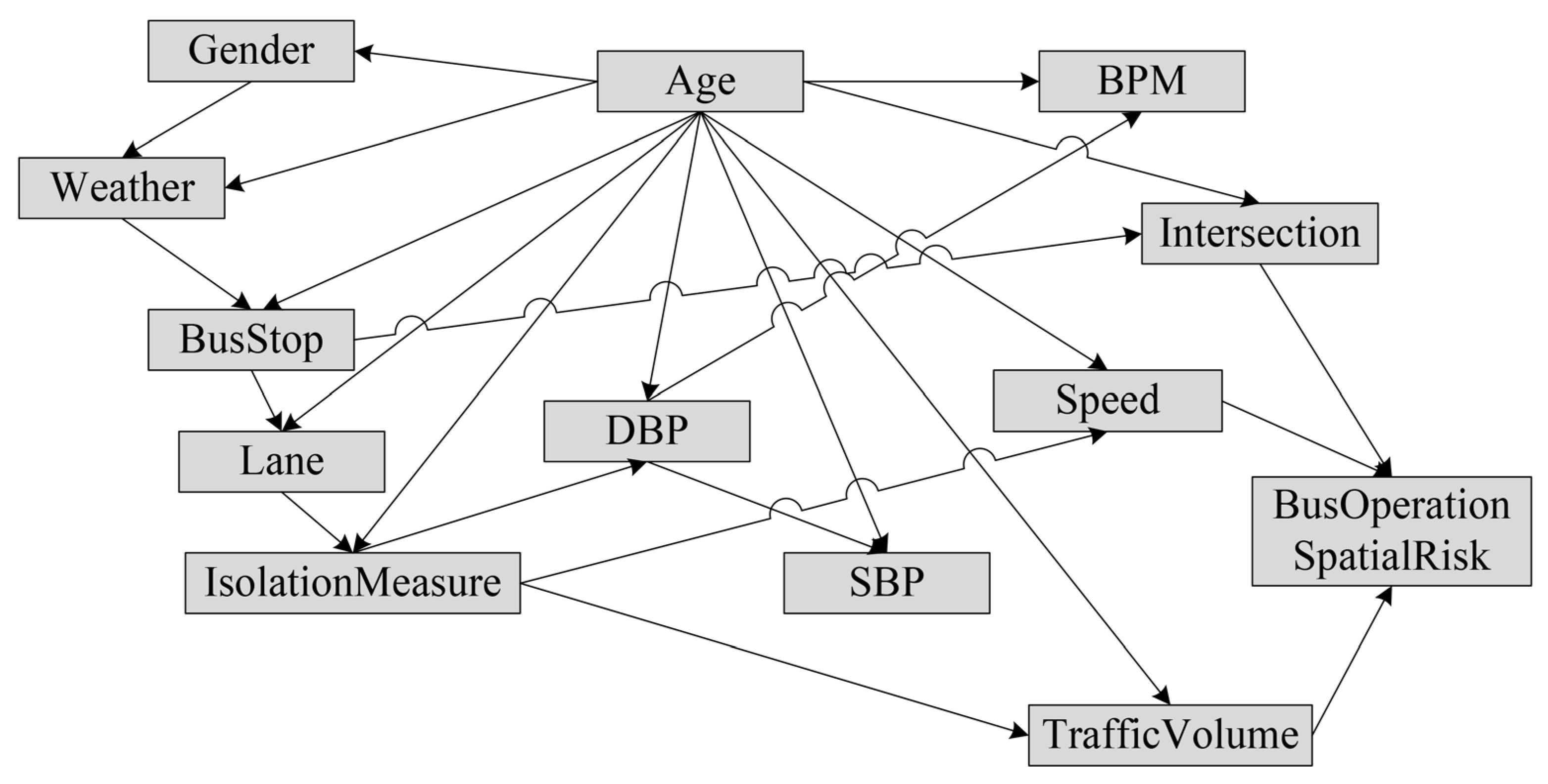
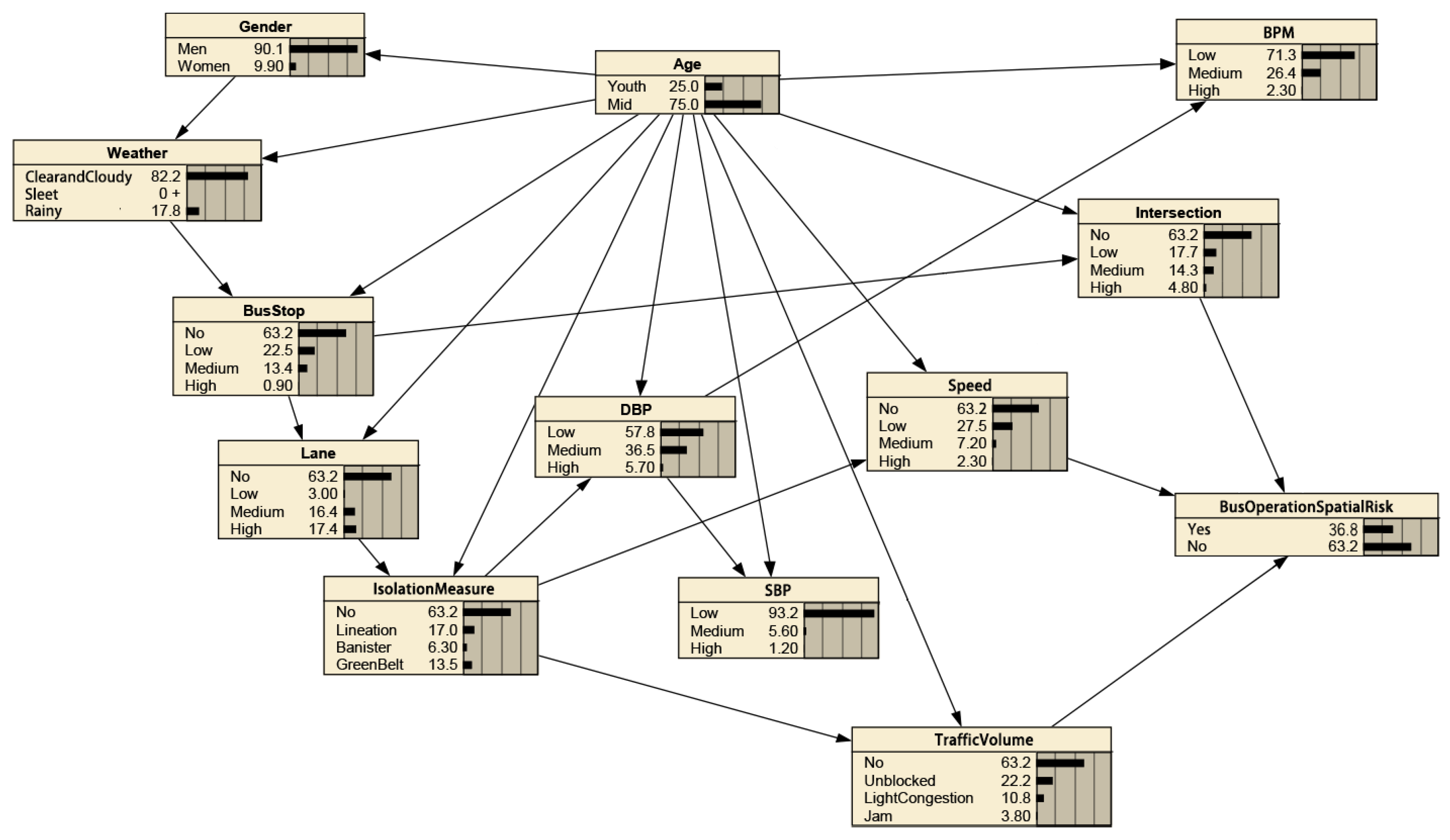
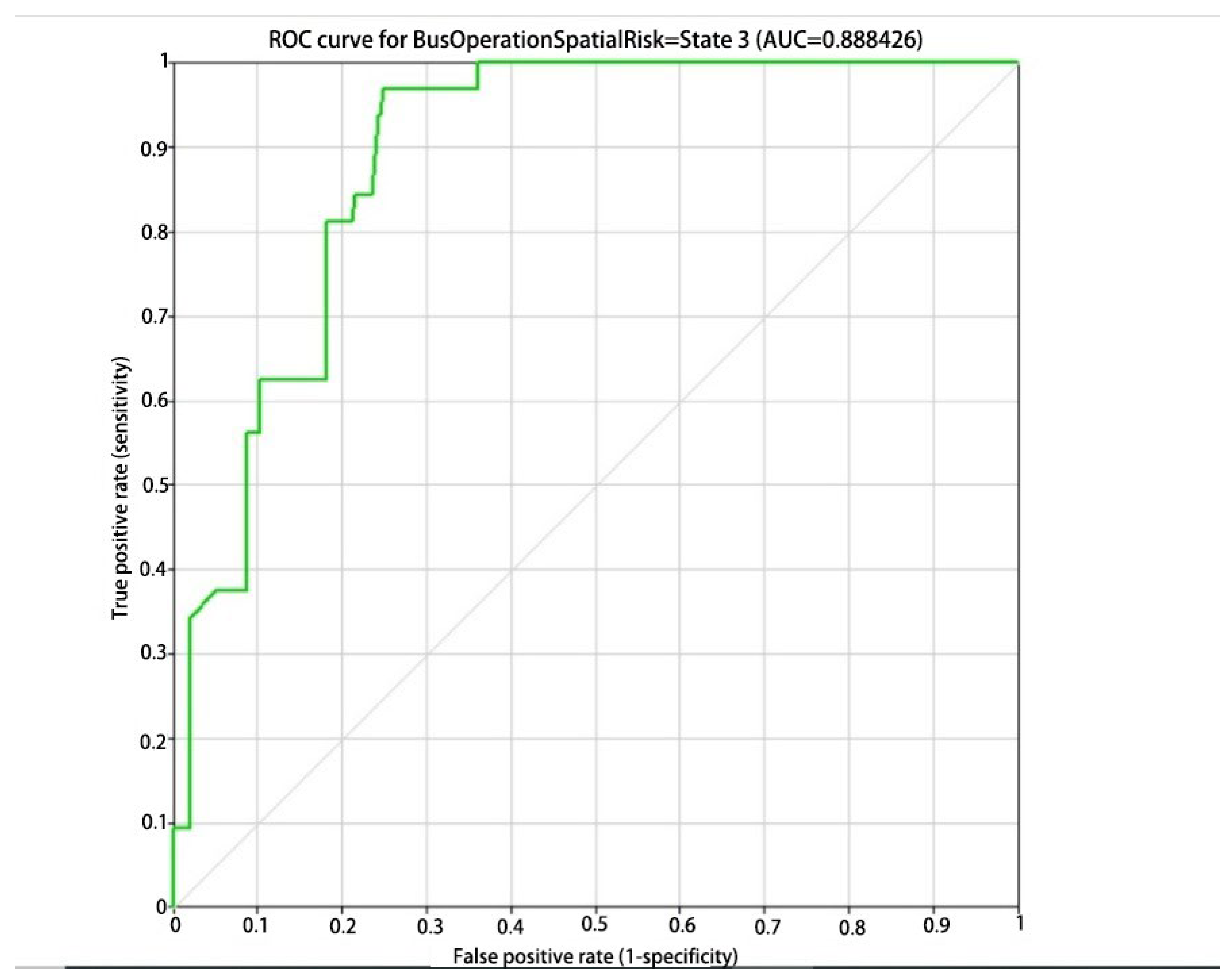
3. Results
4. Discussion
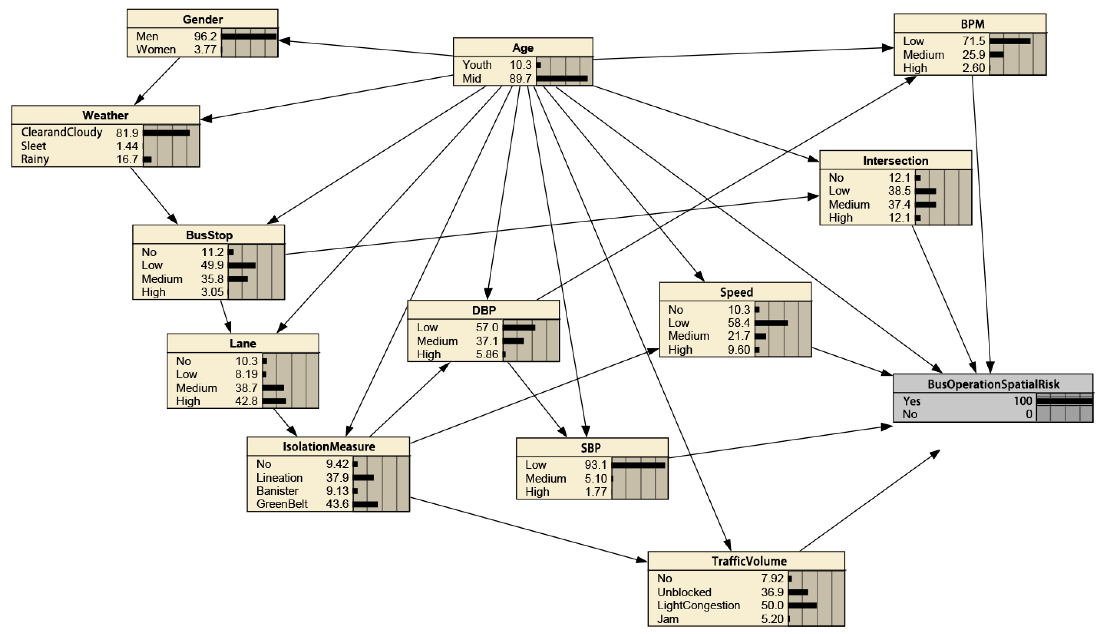
4.1. Backward Reasoning
4.2. Most Probable Explanation
4.3. Sensitivity Analysis
5. Limitations
6. Conclusions
Author Contributions
Funding
Institutional Review Board Statement
Informed Consent Statement
Data Availability Statement
Conflicts of Interest
References
- Inventory of U.S. Greenhouse Gas Emissions and Sinks: 1990–2019. Fed. Regist./FIND 2021, 86, 9339.
- Liu, Z.; Deng, Z.; David, S.J.; Ciais, P. Global carbon emissions in 2023. Nat. Rev. Earth Environ. 2024, 5, 253–254. [Google Scholar] [CrossRef]
- Lah, O. The barriers to low-carbon land-transport and policies to overcome them. Eur. Transp. Res. Rev. 2015, 7, 5. [Google Scholar] [CrossRef]
- Van Fan, Y.; Perry, S.; Klemeš, J.J.; Lee, C.T. A review on air emissions assessment: Transportation. J. Clean. Prod. 2018, 194, 673–684. [Google Scholar] [CrossRef]
- Moktadir, M.A.; Ren, J.Z. Towards green logistics: An innovative decision support model for zero-emission transportation modes development. Transp. Res. Part E 2024, 189, 103648. [Google Scholar] [CrossRef]
- Hassouna, F.M.A.; Assad, M. Towards a Sustainable Public Transportation: Replacing the Conventional Taxis by a Hybrid Taxi Fleet in the West Bank, Palestine. Int. J. Environ. Res. Public Health 2020, 17, 8940. [Google Scholar] [CrossRef]
- Hassouna, F.M.A. Urban Freight Transport Electrification in Westbank, Palestine: Environmental and Economic Benefits. Energies 2022, 15, 4058. [Google Scholar] [CrossRef]
- Fady, M.A. Sustainability assessment of public bus transportation sector in westbank, Palestine. Environ. Res. Commun. 2023, 5, 015001. [Google Scholar]
- Ahangari, H.; Atkinson-Palombo, C.; Garrick, N.W. Assessing the Determinants of Changes in Traffic Fatalities in Developed Countries. Transp. Res. Rec. J. Transp. Res. Board 2015, 2513, 63–71. [Google Scholar] [CrossRef]
- Hassan, H.M.; Al-Faleh, H. Exploring the risk factors associated with the size and severity of roadway crashes in Riyadh. J. Saf. Res. 2013, 47, 67–74. [Google Scholar] [CrossRef]
- Sun, J.; Li, T.N.; Li, F.; Chen, F. Analysis of safety factors for urban expressways considering the effect of congestion in Shanghai, China. Accid. Anal. Prev. 2016, 95, 503–511. [Google Scholar] [CrossRef] [PubMed]
- Sohail, A.; Cheema, M.A.; Ali, M.E.; Toosi, A.N.; Rakha, H.A. Data-driven approaches for road safety: A comprehensive systematic literature review. Saf. Sci. 2022, 158, 105949. [Google Scholar] [CrossRef]
- Aoonrot, C.; Chunho, Y. Developing evaluation framework for intelligent transport system on public transit in Bangkok Metropolitan Regions using fuzzy AHP. Infrastructures 2021, 6, 182. [Google Scholar]
- Kitali, A.E.; Kadeha, C.F.; Kutela, B.; Kidando, E.; Semu, D.D.; Novat, N.; Matyenyi, J.W. Safety evaluation of the first bus rapid transit system in Tanzania. Transp. Res. Rec. J. Transp. Res. Board 2023, 2678, 155–170. [Google Scholar] [CrossRef]
- Luo, S.D.; Leung, A.P.; Qiu, X.Z.; Chan, J.Y.K.; Huang, H.Z. Complementary deep and shallow learning with boosting for public transportation safety. Sensors 2020, 20, 4671. [Google Scholar] [CrossRef]
- Zou, X.; Yue, W.L. A Bayesian Network Approach to Causation Analysis of Road Accidents Using Netica. J. Adv. Transp. 2017, 2017, 2525481. [Google Scholar] [CrossRef]
- Liu, Y.Q.; Wang, X.Y. The Analysis of Driver’s Behavioral Tendency Under Different Emotional States Based on a Bayesian Network. IEEE Trans. Affect. Comput. 2023, 14, 165–177. [Google Scholar] [CrossRef]
- Yang, Z.L.; Yang, Z.S.; Smith, J.; Robert, B.A.P. Risk analysis of bicycle accidents: A Bayesian approach. Reliab. Eng. Syst. Saf. 2021, 209, 107460. [Google Scholar] [CrossRef]
- Ye, F.F.; Yang, L.H.; Wang, Y.M.; Lu, H.T. A data-driven rule-based system for China’s traffic accident prediction by considering the improvement of safety efficiency. Comput. Ind. Eng. 2023, 176, 108924. [Google Scholar] [CrossRef]
- Chen, Y.B.; Zou, Y.J.; Kong, X.Q.; Wu, L.T. Investigating the impact of influential factors on crash types for autonomous vehicles at intersections. J. Transp. Saf. Secur. 2023, 16, 1089–1116. [Google Scholar] [CrossRef]
- Wang, Y.H.; Zhang, J.Y.; Wu, G.S. Bayesian-Based Traffic Safety Evaluation Study for Driverless Infiltration. Appl. Sci. 2023, 13, 12291. [Google Scholar] [CrossRef]
- Jensen, F.V.; Nielsen, T.D. Bayesian Networks and Decision Graphs; Springer Science & Business Media: Berlin/Heidelberg, Germany, 2009. [Google Scholar] [CrossRef]
- Najaf, P.; Thill, J.-C.; Zhang, W.; Fields, M.G. City-level urban form and traffic safety: A structural equation modeling analysis of direct and indirect effects. J. Transp. Geogr. 2018, 69, 257–270. [Google Scholar] [CrossRef]
- Lord, D.; Washington, S.P.; Ivan, J.N. Poisson, Poisson-gamma and zero-inflated regression models of motor vehicle crashes: Balancing statistical fit and theory. Accid. Anal. Prev. 2005, 37, 35–46. [Google Scholar] [CrossRef]
- Martin, J. Relationship between crash rate and hourly traffic flow on interurban motorways. Accid. Anal. Prev. 2002, 34, 619–629. [Google Scholar] [CrossRef]
- Chang, L.Y.; Chen, W.C. Data mining of tree-based models to analyze freeway accident frequency. J. Saf. Res. 2005, 36, 365–375. [Google Scholar] [CrossRef]
- Sullman, M.J.; Meadows, M.L.; Pajo, K.B. Aberrant driving behaviours amongst New Zealand truck drivers. Transp. Res. Part F Traffic Psychol. Behav. 2002, 5, 217–232. [Google Scholar] [CrossRef]
- Kim, J.-K.; Kim, S.; Ulfarsson, G.F.; Porrello, L.A. Bicyclist injury severities in bicyclemotor vehicle accidents. Accid. Anal. Prev. 2007, 39, 238–251. [Google Scholar] [CrossRef]
- Zhao, M.J.; Ji, S.W.; Zhao, Q.R.; Chen, C.; Wei, Z.L. Risk Influencing Factor Analysis of Urban Express Logistics for Public Safety: A Chinese Perspective. Math. Probl. Eng. 2020, 2020, 4571890. [Google Scholar] [CrossRef]
- Chickering, M.D.; Heckerman, D.; Meek, C. Large-sample learning of Bayesian networks is NP-hard. J. Mach. Learn. Res. 2004, 5, 1287–1330. [Google Scholar]
- Sun, L.J.; Lu, Y.; Jin, J.G.; Lee, D.H.; Axhausen, K.W. An integrated Bayesian approach for passenger flow assignment in metro networks. Transp. Res. Part C Emerg. Technol. 2015, 52, 116–131. [Google Scholar] [CrossRef]
- Kim, J.; Wang, G. Diagnosis and prediction of traffic congestion on urban road networks using Bayesian networks. Transp. Res. Rec. J. Transp. Res. Board 2016, 2595, 108–118. [Google Scholar] [CrossRef]
- Wei, T.Z.; Zhu, T.; Bai, H.; Zhao, L.; Wang, X.G. Effects of Driver Gender, Driving Experience, and Visibility on Car-Following Behavior. Transp. Res. Rec. 2024. [Google Scholar] [CrossRef]
- Lyu, N.C.; Duan, Z.C.; Ma, C.X.; Wu, C.Z. Safety margins—A novel approach from risk homeostasis theory for evaluating the impact of advanced driver assistance systems on driving behavior in near-crash events. J. Intell. Transp. Syst. 2021, 25, 93–106. [Google Scholar] [CrossRef]
- Jing, L.L.; Shan, W.; Zhang, Y.Y. Risk preference, risk perception as predictors of risky driving behaviors: The moderating effects of gender, age, and driving experience. J. Transp. Saf. Secur. 2022, 15, 467–492. [Google Scholar] [CrossRef]
- Kim, W.; But, J.; Anorve, V.; Kelly-Baker, T. Examining, U.S. drivers’ characteristics in relation to how frequently they engage in speeding on freeways. Transp. Res. Part F Traffic Psychol. Behav. 2022, 85, 195–208. [Google Scholar] [CrossRef]
- De Vos, B.; Cuenen, A.; Ross, V.; Dirix, H.; Brijs, K.; Brijs, T. The Effectiveness of an Intelligent Speed Assistance System with Real-Time Speeding Interventions for Truck Drivers: A Belgian Simulator Study. Sustainability 2023, 15, 5226. [Google Scholar] [CrossRef]
- Becker, N.; Rust, H.W.; Ulbrich, U. Weather impacts on various types of road crashes: A quantitative analysis using generalized additive models. Eur. Transp. Res. Rev. 2022, 14, 37. [Google Scholar] [CrossRef]
- Li, G.L.; Li, Y.Q.; Craig, B.; Liu, X.Y. Investigating the effect of contextual factors on driving: An experimental study. Transp. Res. Part F Psychol. Behav. 2022, 88, 69–80. [Google Scholar] [CrossRef]


| Independent Variable | Description | Classification | |
|---|---|---|---|
| Driver | Gender | Gender of driver | Men = Men, Women = Women |
| Age | Age of driver | (20, 30] = Youth, (30, 40] = Mid | |
| SBP | Systolic pressure of driver | (100, 115] = Low, (115, 130] = Medium, (130, 145] = High | |
| DBP | Diastolic pressure of driver | (63, 73] = Low, (73, 83] = Medium, (83, 93] = High | |
| BPM | Heart Beats per minute of driver | (59, 75] = Low, (75, 91] = Medium, (91, 107] = High | |
| Vehicle | Speed | Instantaneous speed of bus | (30, 43] = Low, (43, 56] = Medium, (56, 69] = High |
| Road | Lane | Number of road lanes at the time of warning | [1, 2] = Low, (2, 4] = Medium, (4, 8] = High |
| Traffic Volume | Traffic volume at the time of warning | Unblocked = Unblocked, Light congestion = LightCongestion, Jam = Jam | |
| Isolation Measure | Road isolation measures at the time of warning | Lineation = Lineation, Banister = Banister, Green belt = GreenBelt | |
| Bus stop | Number of bus stops on the road at the time of warning | [0, 18] = Low, (18, 36] = Medium, (36, 54] = High | |
| Intersection | Number of road intersections at the time of warning | [0, 8] = Low, (8, 15] = Medium, (15, 22] = High | |
| Environment | Weather | Weather at the time of warning | Sunny or cloudy = ClearandCloudy, Sleet = Sleet, Rainy = Rainy |
| Statistical Indicators | Mean | Std | Min | Max | |
|---|---|---|---|---|---|
| Driver | Age (Years) | 40.5 | 6.06 | 32 | 50 |
| SBP (mmHg) | 118 | 5.73 | 106 | 149 | |
| DBP (mmHg) | 75 | 4.64 | 64 | 94 | |
| BPM (Per minute) | 74 | 7.56 | 57 | 117 | |
| Vehicle | Speed (Km/h) | 39.9 | 8.40 | 30 | 63 |
| Road | Lane | 5 | 1.35 | 1 | 8 |
| Bus stop | 14 | 10.17 | 0 | 53 | |
| Intersection | 8 | 4.38 | 1 | 22 |
| Age (Youth) | Age (Mid) | |
|---|---|---|
| DBP (Low) | 0.466 | 0.656 |
| DBP (Medium) | 0.477 | 0.219 |
| DBP (High) | 0.057 | 0.125 |
| Index | Accuracy | MSE | RMSE | MAE | |
|---|---|---|---|---|---|
| Model | |||||
| BN | 70.0% | 0.416 | 0.645 | 0.335 | |
| RF | 68.6% | 0.449 | 0.670 | 0.355 | |
| SVM | 66.4% | 0.557 | 0.746 | 0.409 | |
| Level | (%) | (%) | (%) | (%) | |
|---|---|---|---|---|---|
| Variable | |||||
| Age | −14.7 | +14.7 | − | − | |
| Gender | +6.1 | −6.13 | − | − | |
| SBP | −52.7 | +30.9 | +14.5 | +7.3 | |
| DPB | −0.1 | −0.5 | +0.57 | − | |
| BPM | −0.8 | +0.6 | +0.16 | − | |
| Speed | +0.2 | −0.5 | +0.3 | − | |
| Lane | −52 | +27.4 | +22.4 | +2.15 | |
| Traffic volume | −52.9 | +5.19 | +22.3 | +25.4 | |
| Isolation measure | −51.3 | +20.8 | +23.1 | +7.3 | |
| Bus stop | −53.78 | +20.9 | +2.83 | +30.1 | |
| Intersections | −55.28 | +14.7 | +39.2 | +1.4 | |
| Weather | −0.3 | +1.44 | −1.1 | − | |
| Variable | MPE |
|---|---|
| Age | 30–40 years |
| Gender | Men |
| SBP | 100–115 mm Hg |
| DPB | 63–73 mm Hg |
| BPM | 59–75 beats/min |
| Speed | 30–43 km/h |
| Lane | 2–4 |
| Traffic volume | Unblocked |
| Isolation measure | Line isolation |
| Bus stop | 0–18 |
| Intersection | 0–8 |
| Weather | Clear and cloudy |
| Node | Mutual Information | Percentage | Variance Credibility |
|---|---|---|---|
| Bus operation spatial risk | 1.329 | 100 | 0.311 |
| Speed | 0.780 | 58.7 | 0.143 |
| Traffic volume | 0.775 | 58.3 | 0.140 |
| Isolation measure | 0.771 | 58 | 0.139 |
| Intersection | 0.769 | 57.9 | 0.139 |
| Bus stop | 0.767 | 57.7 | 0.139 |
| Lane | 0.766 | 57.6 | 0.139 |
| SBP | 0.011 | 0.799 | 0.001 |
| DBP | 0.007 | 0.559 | 0.000 |
| BPM | 0.006 | 0.451 | 0.000 |
| Age | 0.006 | 0.414 | 0.001 |
| Weather | 0.003 | 0.188 | 0.001 |
Disclaimer/Publisher’s Note: The statements, opinions and data contained in all publications are solely those of the individual author(s) and contributor(s) and not of MDPI and/or the editor(s). MDPI and/or the editor(s) disclaim responsibility for any injury to people or property resulting from any ideas, methods, instructions or products referred to in the content. |
© 2024 by the authors. Licensee MDPI, Basel, Switzerland. This article is an open access article distributed under the terms and conditions of the Creative Commons Attribution (CC BY) license (https://creativecommons.org/licenses/by/4.0/).
Share and Cite
Li, H.; Yu, S.; Deng, S.; Ji, T.; Zhang, J.; Mi, J.; Xu, Y.; Liu, L. Identification of Risk Factors for Bus Operation Based on Bayesian Network. Appl. Sci. 2024, 14, 9602. https://doi.org/10.3390/app14209602
Li H, Yu S, Deng S, Ji T, Zhang J, Mi J, Xu Y, Liu L. Identification of Risk Factors for Bus Operation Based on Bayesian Network. Applied Sciences. 2024; 14(20):9602. https://doi.org/10.3390/app14209602
Chicago/Turabian StyleLi, Hongyi, Shijun Yu, Shejun Deng, Tao Ji, Jun Zhang, Jian Mi, Yue Xu, and Lu Liu. 2024. "Identification of Risk Factors for Bus Operation Based on Bayesian Network" Applied Sciences 14, no. 20: 9602. https://doi.org/10.3390/app14209602
APA StyleLi, H., Yu, S., Deng, S., Ji, T., Zhang, J., Mi, J., Xu, Y., & Liu, L. (2024). Identification of Risk Factors for Bus Operation Based on Bayesian Network. Applied Sciences, 14(20), 9602. https://doi.org/10.3390/app14209602