A Loose Integration of High-Rate GNSS and Strong-Motion Records with Variance Compensation Adaptive Kalman Filter for Broadband Co-Seismic Displacements

Abstract

The loose integration system of high-rate GNSS and strong-motion records based on Kalman filtering technology is currently a research focus for capturing broadband co-seismic displacements. To address the problem of time-varying system noise variance in the standard Kalman filter (SKF), a variance compensation adaptive Kalman filter (VC-AKF) was adopted in this study to obtain more accurate high-precision broadband co-seismic displacement and provide reliable data support for seismic scientific research and practical applications. The algorithm continuously updates the system noise variance and calculates the state vector by collecting prediction residuals in real time. To verify the effectiveness and superiority of this method, a numerical simulation and a seismic experiment from the 2017 Ms 7.0 Jiuzhaigou earthquake were carried out for comparative analysis. Based on the simulation results, the precision of the proposed algorithm was 46% higher than that of the SKF. The seismic experiment results indicate that the proposed VC-AKF approach can eliminate the baseline shift of accelerometers and weaken the influence of time-varying system noise variance towards more robust displacement information.

1. Introduction

More than 16 countries worldwide have developed and implemented earthquake early warning (EEW) systems, with some systems already providing warnings to the public, while others are still in testing phases. Japan was a pioneer in the 1960s with the development of the UrEDAS system based on traditional seismology, which was put into operation in 1992 and performed well for small to medium-sized earthquakes. However, the system struggled with accurate magnitude estimation for large earthquakes (Mw > 7.0), as demonstrated during the Mw 9.0 earthquake in 2011, where UrEDAS’s preliminary magnitude estimates were significantly lower than the actual magnitude, leading to delays in defensive measures. Recent research indicates that incorporating GPS stations can substantially enhance the accuracy and timeliness of earthquake warnings for large events.

Co-seismic displacement is a crucial prerequisite for estimating earthquake magnitude. Accurate co-seismic displacement is key to determining focal depth, epicenter location, and magnitude, significantly enhancing the accuracy and timeliness of earthquake early warnings. In traditional earthquake monitoring, the observed values from strong-motion (SM) seismometers are acceleration data, which have the advantage of not being constrained by amplitude in near-field conditions. However, during large earthquakes, these instruments can be affected by ground motion, leading to tilting and rotation, which causes baseline drift [1,2,3]. Therefore, Vladimir Graizer and others found that the displacement calculated by double integration of acceleration includes short-term white noise and long-term disturbances, making it difficult to ensure the reliability of the data. [4,5]. Although many empirical baseline correction methods have been proposed to remove deviations, the processed signals still cannot accurately capture the permanent displacement of the measurement station [6]. And it is difficult to ensure timeliness. For instance, relying on SM (strong motion) measurements, the initial warning during the Mw 9.0 Great East Japan Earthquake on 11 March 2011 was issued a mere 25.8 s post-quake, citing a magnitude of 7.2. This estimate was subsequently revised to 8.1 two minutes later, and it took a further three hours for the magnitude to be refined to Mw 8.8. Compared to the final determination of Mw 9.0 by the Japan Meteorological Agency, the magnitude was significantly underestimated, which consequently led to a delayed deployment of appropriate defensive measures. In contrast, Colombelli et al. used SM sensors and GPS for early warning. The SM sensor detected anomalies 15 s after the quake, while the GPS detected the event after the S-wave arrived, but it estimated the magnitude as Mw 8.9 just two minutes later, showing the reliability and timeliness of using GPS data for magnitude estimation in major earthquakes [7].

In some areas, GPS signals can be obstructed by physical barriers, which affects data quality. Additionally, there may be a brief delay in GPS systems following an earthquake, as it takes time for GPS satellites and receivers to process and transmit data. Global navigation satellite systems (GNSSs), by integrating multiple satellite systems, enhance global coverage and positioning accuracy. They also excel in real-time data processing, providing more timely positioning information, which is particularly important for earthquake monitoring and early warning systems [8,9,10,11]. To address the above issues, high-rate GNSS technology is being employed for monitoring crustal deformation. With the refinement of GNSS-related hardware performance and GNSS observation processing methods, especially for the maturity of single-epoch instantaneous positioning technology, GNSS seismology has gradually extended from long-term continuous static displacement estimation to short-term dynamic motion monitoring [12,13,14]. Consequently, GNSSs have been widely applied in the field of seismic rupture process calculation [15,16,17,18], fault slip model inversion [19,20], rapid magnitude estimation [21,22,23], and real-time earthquake early warning (EEW) [24,25]. In general, SM observations provide acceleration information and have the advantage of capturing unlimited near-field amplitude, allowing for high-frequency monitoring of short-duration intense shaking. This offers extremely important information for earthquake research; however, during strong shaking in large earthquakes, SM can be easily affected by surface motion. Compared with SM, one of the advantages of high-rate GNSSs is measuring ground displacements directly without drifts in an absolute reference frame [26]. Even in cases of (extra)large earthquakes, they can record more accurate displacements to estimate more precise magnitude. However, there are still several constraints and challenges for co-seismic displacement measurements with high-rate GNSSs. (1) During measurement, high-rate GNSSs are insensitive to weak surface deformation and do not pick up the primary seismic wave easily [9]. (2) Restricted by the bandwidth of receivers, high-rate GNSSs cannot achieve a sampling rate comparable to that of SM accelerometers (200 Hz or even 400 Hz) [27,28,29]. Therefore, SM accelerometers and high-rate GNSSs complement each other. By integrating and analyzing them together, it is possible to obtain high-precision positional information and high-sampling-rate broadband co-seismic displacement, thereby improving the accuracy and reliability of earthquake early warning systems.

To maximize the advantages and minimize the weaknesses of SM accelerations and high-rate GNSSs, many methods have been proposed to combine GNSS displacements and SM accelerations at co-located sites. Emore et al. [30] used a numerical inversion approach that considered the baseline shift in SM accelerations to estimate co-seismic displacements with the constraint of GNSS data. Wang et al. [31] used linear trigonometric and time correlation to express the baseline shift in SM accelerations, and obtained the best fit with high-rate GNSS displacements. However, the above techniques were not employed for real-time applications because of their subjective process. Tu et al. [32] derived the baseline shift in SM accelerations by comparing single-frequency GNSS displacements without pre-event trends or acceleration-integrated displacements, whereas the single-frequency GNSS was not suitable for long-term monitoring. At present, Kalman filters and particle filters (PFs) are popular research solutions for retrieving optimal estimates of co-seismic displacements in high-rate GNSS–SM accelerometer integration systems. In complex earthquake monitoring scenarios, such as when seismic waves propagate through different geological layers, the resulting displacement and acceleration can be affected by various nonlinear effects. PFs can be applied to estimate nonlinear dynamic systems. The use of PFs is a Bayesian method of estimating state variables in dynamic systems, particularly when dealing with nonlinearities and non-Gaussian noise. It approximates the posterior probability of the state using random samples (particles). But PFs require a large number of particles for accurate estimates, leading to increased computational and storage demands, especially in high-dimensional systems. The method is also sensitive to the distribution of initial particles, with improper initialization potentially causing biased results. Additionally, the performance of the PF method depends on the choice of parameters, such as the number of particles and resampling strategies [33,34,35,36]. The Kalman filter not only supports real-time applications but also implicitly and automatically corrects baseline shifts in SM data. Smyth and Wu [37] proposed a loose integration method by the standard Kalman filter (SKF) that considered GNSS displacements as observation quantities and SM accelerations as control quantities. Bock et al. [38] adopted the SKF to estimate broadband dynamic co-seismic displacements for shake-table experiments and the 2010 El Mayor–Cucapah earthquake. Shu et al. [39] revised the SKF to obtain integrated waveforms and eliminate the aliasing problem existing in the 1 Hz GNSS signals of GSIS. Song and Xu [40] upgraded the loose integration method with two parallel SKFs to decrease the influence of GNSS colored noise with uneven energy distribution across the frequency spectrum, in contrast to traditional Gaussian white noise. This includes commonly encountered types such as pink noise, blue noise, and red noise. Alternatively, there are also several tight integration methods by Kalman filters that add SM accelerations into the normal equation of GNSS positioning to improve resolving ambiguities [27,41,42,43].

However, the optimality of the Kalman filter solution is determined largely by a priori knowledge of the noise statistics. The use of incorrect a priori knowledge may result in inaccurate estimation or even filter divergence. In GSIS, the observation noise variance from a GNSS is relatively easy to acquire and is comparatively homogeneous over a long period of time. Nevertheless, the system noise variance from SM is prone to nonlinear time variation because of its rotation and tilts, which means it is not suitable to fix to a certain a priori value. Therefore, the Rauch–Tung–Striebel (RTS) smoother and the adaptive Kalman filter (AKF) have been used to solve this problem [44,45]. The RTS smoothing technique estimates the state minimum variance by all the output data in a fixed interval to reduce the effect of the time-varying system noise variance. Although the accuracy of results can be further improved, the RTS smoother is a causal system and requires more computational time and resources. The AKF methods have the benefits of determining and correcting incorrect state vectors and the statistical characteristics of system noise appropriately, which can be generally classified into four methods: Bayesian, maximum likelihood, correlation, and covariance matching. The Bayesian and maximum likelihood methods are based on probability statistics to calculate noise covariance. In the calculation, all data need to be used for multiple iterations, resulting in these methods being relatively cumbersome and inefficient for GSIS [46,47]. The correlation method estimates the steady-state filter gain and the noise covariance from the autocorrelation function of the observation data or the innovation sequence. Because of the requirement of large data windows, the correlation method has high processing load. In addition, it is difficult to guarantee the positive definiteness of matrices, leading to biased results. In contrast, the covariance matching method is a recursive algorithm in real time that calculates a closer approximation to the actual state valuation by estimating the system noise variance vector with its own information [48,49]. Compared with the other AKF methods, the covariance matching method is more compatible with the time-varying characteristics of the system noise in GSIS, and has unique advantages at data fusion for real-time applications and simple computation.

In order to deal with the problem of the time-varying system noise variance from SM, a new AKF approach—variance compensation adaptive Kalman filter (VC-AKF)—is presented in this study to construct the loose integration of high-rate GNSS and SM records. VC-AKF is a covariance matching method that uses predicted residuals to estimate system noise covariance vectors in real time, and then substitutes valuations into the filtering process to correct original system noise covariance. The remaining chapters of this paper are organized as follows. First, the high-rate GNSS and SM loose integration system model is introduced, and the method based on VC-AKF is described particularly. Then, a simulation experiment is used to validate the effectiveness and robustness of the presented VC-AKF, and the 2017 Jiuzhaigou Ms 7.0 earthquake is taken as an application to retrieval the broadband co-seismic waveforms. The main analysis and conclusions are provided at the end.

2. Materials and Methods

2.1. High-Rate GNSS and SM Loose Integration System Functions

During an earthquake, the ground is treated as a continuous dynamics system. High-frequency GNSS provides absolute three-dimensional displacement information and is not affected by tilt or baseline drift. When tilt occurs in SM (strong-motion accelerometers), the data typically exhibit anomalies in the low-frequency range, as the false acceleration caused by the tilt results in displacement drift that persists even after the shaking stops. GNSS data do not have this kind of low-frequency drift. Therefore, this paper integrates GNSS data to effectively mitigate the impact of tilt effects in SM data on measurement results. The algorithm presented in this paper takes into account and avoids the issue of baseline deviation caused by the tilt and rotation of the SM sensor, which can make it difficult for the integrated displacement data to accurately reflect the true surface displacement. Moreover, once accurate surface displacements in the three directions have been obtained, displacements in other directions can be derived through appropriate angular projections. Due to the mutual independence of each, the state of motions can be defined by the following first-order linear differential equation:

$$x\left(t+1\right)=Ax\left(t\right)+Ba\left(t\right)+C\alpha \left(t\right)$$

(1)

$$x\left(t\right)=\left[\begin{array}{c}d\left(t\right)\\ v\left(t\right)\end{array}\right],A=\left[\begin{array}{cc}0& 1\\ 0& 0\end{array}\right],B=\left[\begin{array}{c}0\\ 1\end{array}\right],C=\left[\begin{array}{c}0\\ 1\end{array}\right]$$

(2)

where the state vector $x\left(t\right)$ consists of the displacement $d\left(t\right)$ and the velocity $v\left(t\right)$. $a\left(t\right)$ is the acceleration. $\alpha \left(t\right)$ is the system noise with distribution $\alpha \left(t\right)\sim \left(0,Q\right)$. The system noise stochastic model is expressed as:

$$Q=\left[\begin{array}{cc}0& 0\\ 0& q\end{array}\right]$$

(3)

In this study, if the above first-order linear differential equation is discretized, its state equation coefficient matrix will be changed. Therefore, it is assumed that the discrete data sampling interval is $\tau$, the discrete GNSS displacement is $z$, and the SM acceleration is $a$. Then, the discrete state equation and observation equation at epoch $k$ can be established as:

$$x_k=A^S{x}_{k-1}+B^S{a}_{k-1}+{\alpha }_{k-1}$$

(4)

and:

$$z_k=H_k{x}_k+{\beta }_k$$

(5)

where $k=1,2,3,\dots ,N^{+}$. The SM acceleration $a_{k-1}$ is regarded as a constant in the equal time sampling interval. $H_k$ is a designed matrix describing the relationship between observations and state vectors. The system noise ${\alpha }_{k-1}$. and the GNSS displacement noise ${\beta }_k$ with a distribution ${\beta }_k\sim \left(0,R\right)$ are observation noises. In Equation (4), the noise derives only from the SM acceleration time series, and thereby the system noise variance matrix is given as follows:

$$Q=\left[\begin{array}{cc}q{\tau }_a^3/3& q{\tau }_a^2/2\\ q{\tau }_a^2/2& q{\tau }_a\end{array}\right]$$

(6)

and the coefficient matrix can be described as:

$$A^S=\left[\begin{array}{cc}1& {\tau }_a\\ 0& 1\end{array}\right],B^S=\left[\begin{array}{c}{\tau }_a^2/2\\ {\tau }_a\end{array}\right]$$

(7)

where $q$ is a priori system noise variance. ${\tau }_a$ is the sampling interval of SM.

In Equation (5), the displacement observations are mainly GNSS displacement time series, and the observation noise variance matrix can be determined as:

$$R={\displaystyle \frac{r}{{\tau }_d}}$$

(8)

where $r$ and ${\tau }_d$ are the variance and sampling interval of GNSS displacements, respectively.

According to Equations (4)–(8), the loose integration system of high-rate GNSS and SM can be established by the SKF.

2.2. Variance Compensation Adaptive Kalman Filter for High-Rate GNSS and SM Loose Integration

The variance compensation method is a recursive algorithm in real time that calculates a closer approximation to the actual state valuation by estimating the system noise variance vector with its own information [48]. According to the analysis of the loose integration, the state one-step prediction equation can be assumed as:

$${\widehat{x}}_k^{-}=A{\widehat{x}}_{k-1}^{-}+B{\alpha }_{k-1}$$

(9)

where the hat notation “ˆ” represents the estimated value of the state vector. The right superscript “ˉ” represents the prior value of the state vector before the update step. Define the corresponding predicted state covariance matrix as:

$$P_k^{-}=A{P}_{k-1}{A}^T+Q$$

(10)

and the filtering gain matrix as:

$$G_k=P_k^{-}{H}^T{[H{P}_k^{-}{H}^T+R]}^{-1}$$

(11)

Then, the state optimal estimation can be written as:

$${\widehat{x}}_k={\widehat{x}}_k^{-}+G_k[z_k-H{\widehat{x}}_k^{-}]$$

(12)

where ${\widehat{x}}_k$ is the filter value, and $z_k-H{\widehat{x}}_k^{-}$ is the forecast residual value. Consequently, the corresponding predicted state covariance matrix is redefined as:

$$P_k=(I-G_{k}H)P_k^{-}$$

(13)

Following Hu et al. [50], the prediction residual is presented as:

$$V_k=z_k-{\widehat{z}}_k$$

(14)

where $z_k$ is the observation vector at epoch $k$, and ${\widehat{z}}_k$ is the best predicted value at epoch $k$. According to Equations (5) and (14), let:

$$E=V_k^T{V}_k-tr(HA{P}_k{A}^T{H}^T)-tr(R)$$

(15)

The estimate of $Q$ can be denoted as:

$$\left\{\begin{array}{l}Q={(O^{T}O)}^{-1}{O}^{T}E\hfill \\ O=HAC\hfill \end{array}\right.$$

(16)

From Equations (15) and (16), VC-AKF can further optimize the loose integration of high-rate GNSS and SM, which not only has the ability to estimate the system noise covariance matrix $Q$ in real time but also can appropriately increase the weight of better-quality GNSS data in the loose integration system when the SM baseline drifts severely. The detailed steps of VC-AKF for high-rate GNSS and SM loose integration can be described as follows.

• Take high-rate GNSS time series displacement and SM time series acceleration as input data.
• Determine the initial value of the VC-AKF model, including: initial state vector $x_0=0$ and its covariance matrix $P_0=I$ and the system noise matrix $Q_0$.
• Build the VC-AKF model according to Equations (4)–(16).
• Calculate the one-step prediction value ${\widehat{x}}_k^{-}$, predicted covariance value $P_k^{-}$ and gain matrix $G_k$.
• Implement the VC-AKF model, calculate and correct the system noise covariance matrix $Q$.
• Return to (4), recursive calculations.
• Obtain the filtered value ${\widehat{x}}_k$ and the covariance matrix $P_k$ after each calculation.

3. Experiments and Results

As previously mentioned, co-seismic displacement reflects the ground displacement during an earthquake and is a key parameter for estimating the earthquake’s magnitude. Co-seismic displacement provides a measure of fault slip, which is directly related to the magnitude. Therefore, accurately obtaining the co-seismic displacement caused by an earthquake can more directly help infer the magnitude. High-frequency GNSS provides absolute three-dimensional displacement information that is not affected by tilt or baseline drift. This makes it a reliable reference for accelerometer data, especially during and after an earthquake, as GNSS displacement data can maintain high accuracy and stability. SM (strong-motion) accelerometers, with their high temporal resolution, can capture high-frequency components of the shaking, including rapid acceleration changes. Since the time resolution of GNSS is relatively low, it may lack sufficient high-frequency information, making SM a good complement to GNSS in capturing high-frequency components. Therefore, this paper integrates GNSS displacement monitoring data with SM instrument acceleration monitoring data to obtain a wideband co-seismic displacement with both high-precision surface displacement information and high sampling rate. To evaluate the performance of the presented VC-AKF in the loose integration system of displacements and accelerations, the simulation experiment and practical seismic application are conducted as follows.

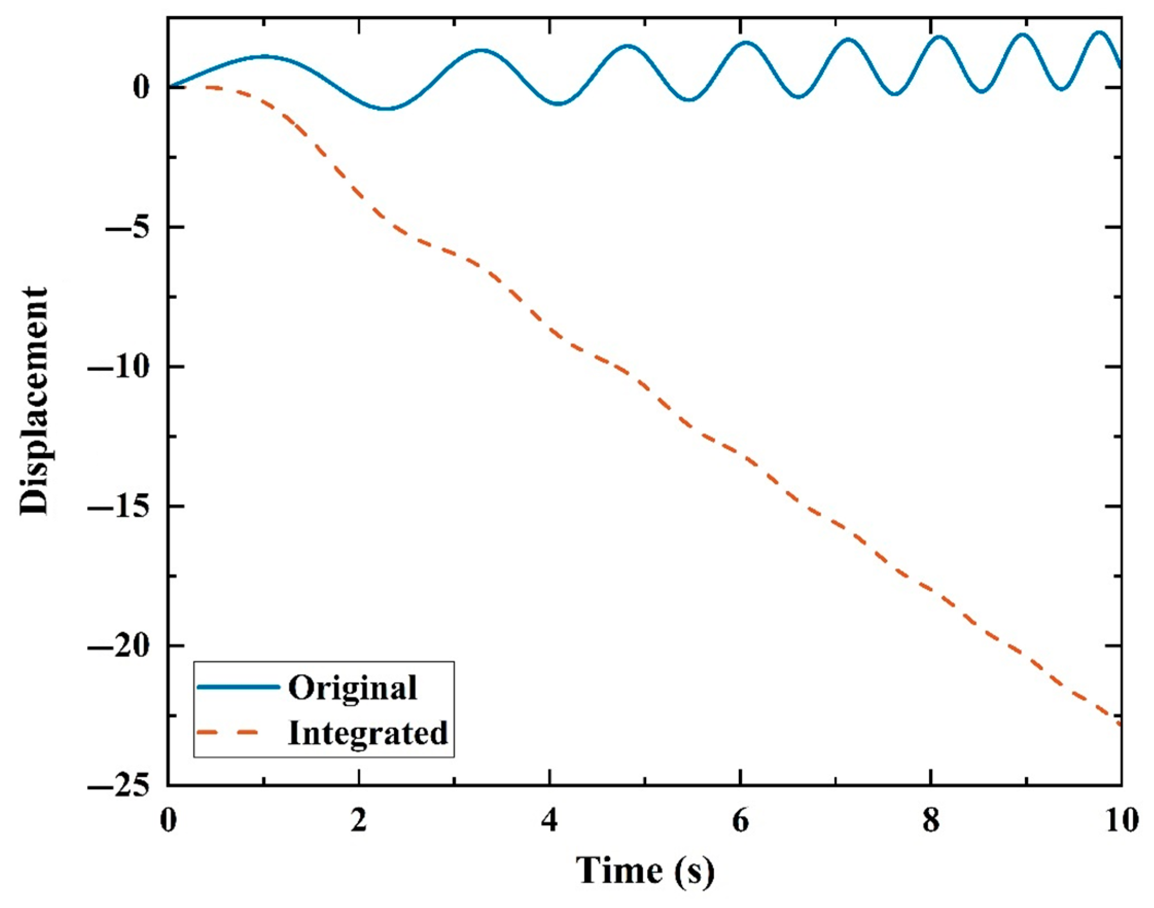
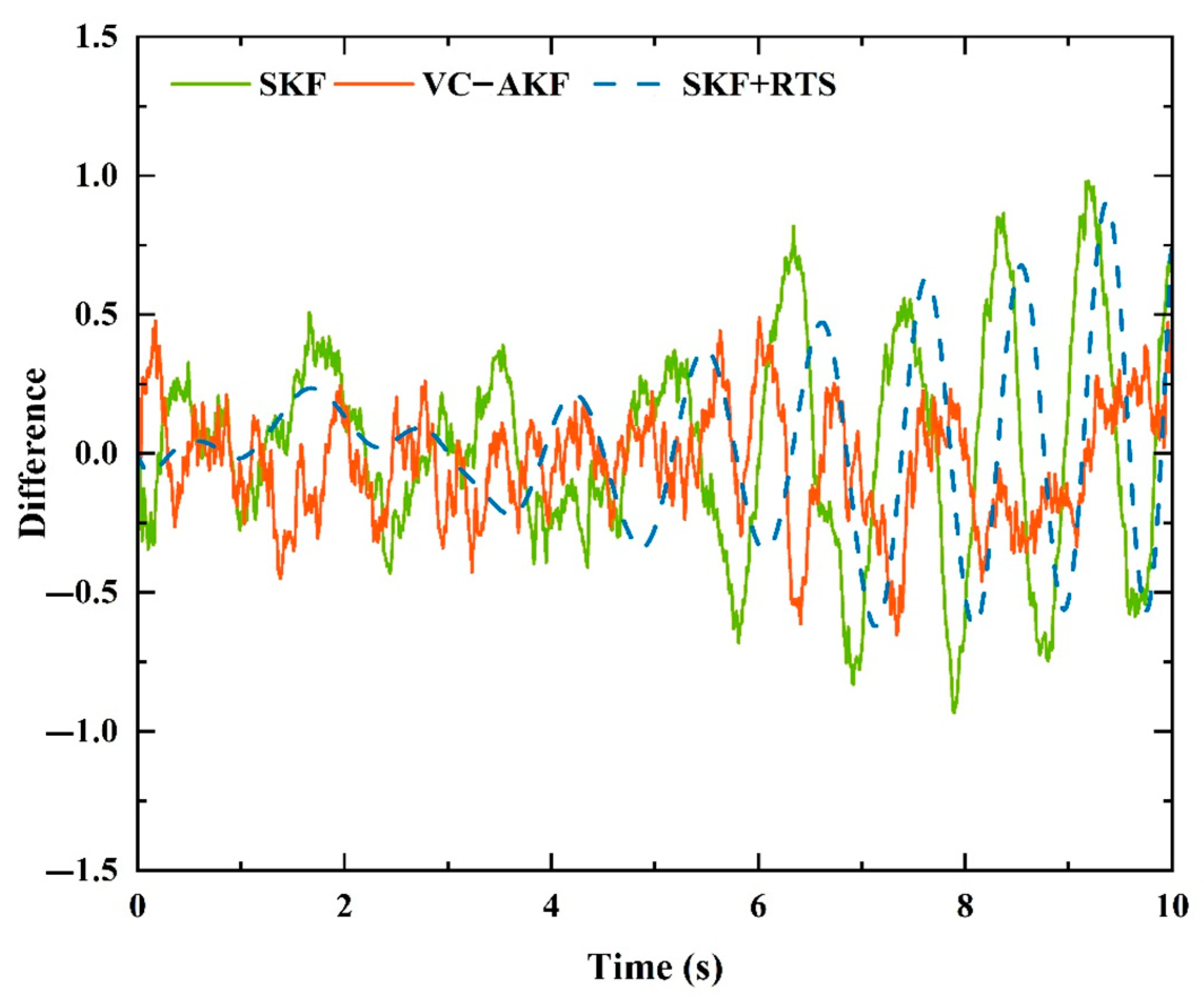
3.1. Simulation Experiment

In this study, the swept sinusoidal signal is adopted to validate the accuracy of the presented VC-AKF, as it can determine whether the proposed method is susceptible to changes in the frequency content of the signal [39]. Assume that the displacement is a sinusoidal swept signal with linear drift, of which time series are as follows:

$$x\left(t\right)=\sin \left[\left(at+b\right)t\right]+ct$$

(17)

where $a=\pi /9,b=2\pi /5,c=0.1$. The time series of the corresponding velocity and acceleration can be obtained by the following formulas:

$$\dot{x}\left(t\right)=\left(2at+b\right)\cos \left[\left(at+b\right)t\right]+c$$

(18)

$$\ddot{x}\left(t\right)=2a\cos \left[\left(at+b\right)t\right]-{\left(2at+b\right)}^2\sin \left[\left(at+b\right)t\right]$$

(19)

As previously mentioned, the data monitored by SM are generally acceleration information. To obtain co-seismic displacement, a double integration is required. Under the presence of linear drift, it may be challenging to accurately recover the actual ground displacement by performing double integration on acceleration data. The impact of linear drift is present in the acceleration information, but after double integration, this linear drift information will be lost. As shown in Equations (17)–(19), the original displacement contains linear drift information, but after obtaining the acceleration information through a second differential, the linear drift information has disappeared. Therefore, in theory, when displacement is obtained by a double integration from acceleration, the linear drift information will also be difficult to recover. To intuitively illustrate this phenomenon, this paper presents a simulated simple linear drift experiment to express that the integration of acceleration information will be difficult to restore the actual displacement. The experimental results are shown in Figure 1. The original displacement time series from the sinusoidal frequency sweep signal and acceleration-derived displacement time series from the acceleration integral are shown in the solid blue line and orange dashed line, respectively. It can be seen that the linear drift in displacements is not recognized by accelerometers after differentiation, which means the linear drift of the original signal cannot be recovered by accelerations after secondary integration. This leads to the loss of linear drift information and makes it difficult to accurately recover the actual ground displacement. To address this issue, this paper proposes combining SM data with high-frequency GNSS data.

Thus, the high-rate GNSS displacement and SM acceleration loose integration will be conducted in this study to acquire displacement with both high-precision and high sampling rate. As this is the simulated experiment, to consider the multi-rate estimation case, it is assumed that the displacement sampling rate is 100 Hz and the acceleration sampling rate is 1000 Hz. In practice, such a high sampling rate is normally unnecessary for most seismic applications. However, it does provide a good data source for mathematical models that require large amounts of data for iterative calculations and capture very-high-frequency sudden response changes. A separate white noise is added to the original displacement and acceleration signals, i.e., $SNR=5$. Initialize the constant noise statistical properties as $q=1,R=0.1$. Since the exact time series of displacements are given, the results can be analyzed by errors from the original signal.

Figure 2 indicates errors of the SKF, VC-AKF, and SKF with RTS smoothing (SKF + RTS). As shown in

Table 1. Root mean square error (RMSE) of displacements by the standard Kalman filter (SKF), variance compensation adaptive Kalman filter (VC-AKF), and standard Kalman filter with Rauch–Tung–Striebel smoothing (SKF + RTS).

Model	RMSE
SKF	0.379
VC-AKF	0.205
SKF + RTS	0.294

, the root mean square error (RMSE) is used as a statistical metric to measure the filter accuracy. The smaller the RMSE, the better the filter effect. Figure 2 and Table 1 highlight the following. (1) The influence of the system’s prior noise covariance parameter on the multi-rate Kalman filter cannot be neglected. As the iterations of the algorithm continuously increase, the SKF results become worse from 5.7 s. Conversely, VC-AKF can effectively overcome problems of filtering divergence and accuracy degradation in SKF. The derived displacements are improved by 46% compared with SKF, which verifies the effectiveness and superiority of the presented VC-AKF approach in this study. (2) SKF + RTS can decrease the errors carried by filtering initial values and increase the estimation precision of the SKF. After smoothing, the accuracy of displacements is improved by 22%, which is less than that of VC-AKF. Moreover, SKF + RTS is incapable of modifying the filter divergence, which indicates that it cannot completely solve the problem of system noise variance variation.

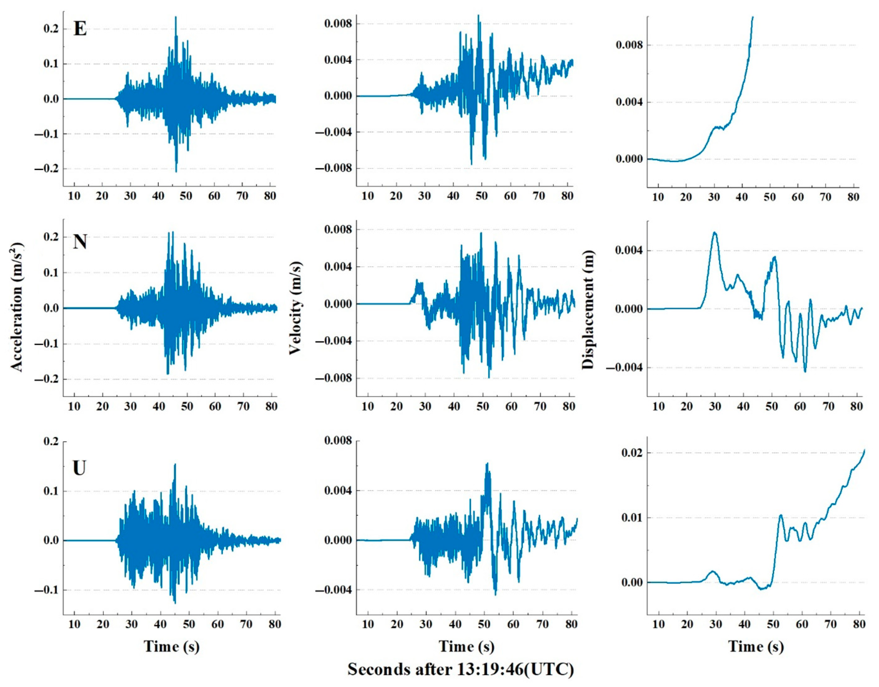
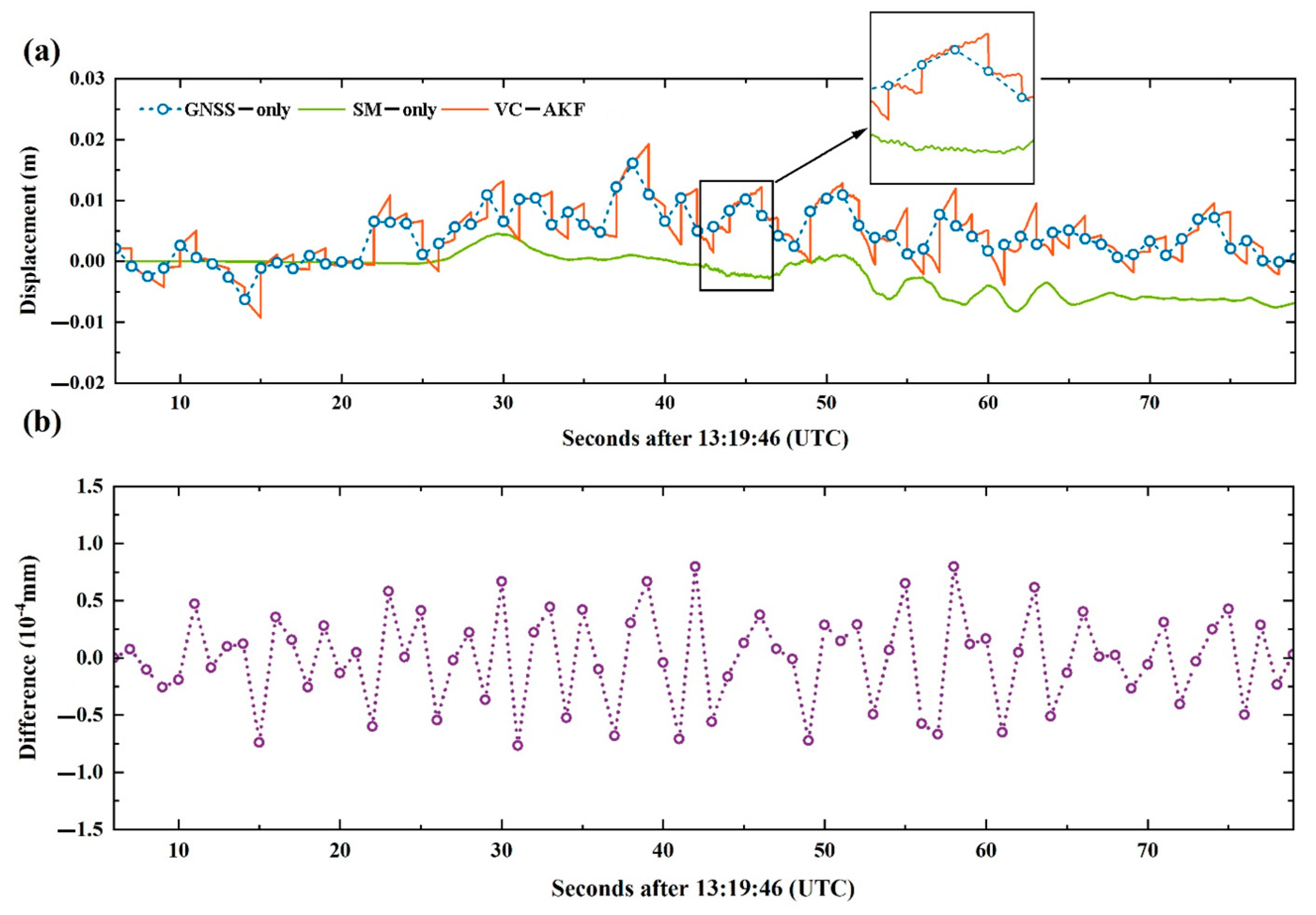
3.2. Application in the 2017 Ms 7.0 Jiuzhaigou Earthquake

The 2017 Ms7.0 Jiuzhaigou earthquake occurred in Sichuan Province of China at 3:19:46 (UTC) on August 8. The epicenter was at 33.20° N, 103.82° E, and the focal depth was about 20 km. After the main shock, a large number of aftershocks occurred successively in the epicenter area, some of which reached a magnitude of 4.0. This earthquake became another magnitude 7.0 earthquake in the eastern part of the Bayan Har block after the 2013 Lushan Ms 7.0 earthquake. In the near-field area of the Jiuzhaigou earthquake, these motions were successfully recorded by several 1 Hz high-rate GNSS observation stations of the GNSS data product service platform of the China Earthquake Administration, and several 200 Hz SM accelerometer observation stations of the China Earthquake Networks Center, National Earthquake Data Center. These seismic monitoring networks provide a large amount of available data to validate the effectiveness and robustness of the proposed method for broadband co-seismic deformation.

To monitor the crustal co-seismic deformation by integrating GNSS and SM data, GSMX and 62MXT are selected as GNSS/SM co-located stations for analysis. The high-rate GNSS and SM station information is shown in

Table 2. Information of high-rate GNSS and strong-motion co-located stations.

Station	Latitude (°)	Longitude (°)	Epicentral Distance (km)	Station Spacing (km)
GSMX	34.43	104.02	137.92	3.80
62MXT	34.40	104.00	134.38

. During the experiment, the data processing time is from 13:19:52 to 13:21:07 (UTC) on 8 August 2017 with a total of 75 s. The observation process is simulated in real time, and the final displacement results are converted into north–south, east–west, and upward directions.

For SM, baseline shifts can be broadly categorized into two groups: baseline shift before the event and baseline shift caused by the event [2]. Theoretically, the acceleration observations should be close to zero before the earthquake wave arrives. However, due to the initial bias caused by unadjusted instruments and ambient temperature changes, the recorded value is nonzero before the event. The resulting error (i.e., initial baseline value) would lead to the integral displacement drift severely if it is not corrected before the event. Therefore, in this study, the first 10 s of basic accelerations are used to estimate the initial baseline value, which is subtracted from the subsequent recordings to remove the baseline shift before the event. Figure 3 shows the acceleration, velocity, and co-seismic displacement time series of 62MXT stations after prior baseline correction during the earthquake in north–south, east–west, and upward directions.

In Figure 3, the velocity is supposed to gradually recover to near zero after the violent shake, but there is some deviation in the actual result due to the ground inclination and rotation. On the other hand, the integral displacement should be fixed at a certain value, but in the second half of the displacement time series, severe drifts occur. From the above analysis, it can be concluded that the original SM acceleration observations not only have the baseline shift before the event, but also contain the baseline shift caused by the event. Therefore, aiming to correct the baseline shift during the earthquake, high-rate GNSS displacement is introduced as an external constraint for data calibration and fusion.

Figure 4 shows the displacement results from 6 s after the main shock. The inspections from this figure highlight the following. (1) The presented VC-AKF has the ability to eliminate the baseline shift caused by the event in real time and better consistency with the GNSS results. Moreover, there is no drift or divergence phenomenon throughout the earthquake, and accurate permanent displacements can be derived. (2) Compared with GNSS, the surface co-seismic deformations can be described in more detail by the proposed VC-AKF. Specifically, the overall trend of the integrated data is constructed by the GNSS displacement, while the details are expressed by the SM acceleration with higher sampling rate. Therefore, VC-AKF can effectively combine the advantages of GNSS and SM, and further capture broadband crustal motion signals directly. (3) The difference between the GNSS-derived and VC-AKF-derived displacements mainly reflects the GNSS noise level, which is within $1\times {10}^{-4}\mathrm{mm}$. This implies that the overall GNSS noise level in the loose integration is relatively stable and homogeneous during the earthquake.

To demonstrate the superiority of the presented VC-AKF in real-time loose integration, Figure 5 shows the comparison of VC-AKF and SKF with different a priori variances $q$ and $100q$. In this study, the variance in the pre-event noise of the accelerometer $q$ is about $6\times {10}^{-5}\mathrm{m}/{\mathrm{s}}^2$ at the 62MXT station. The time value before the system noise variance $q$ mainly depends on the intensity of the station motion in practical applications. Figure 5 clearly highlights the following. (1) It is obvious that the derived results of the SKF are heavily dependent on the input of the system noise variance. When a relatively small system noise variance $q$ is input, the derived results cannot absorb the residual baseline shift of SM well. This problem can be solved by using a larger system noise variance, such as $100q$. As shown in Figure 5a, the derived displacement time series from SKF-100q are more similar to those of VC-AKF compared to SKF-q, which means that VC-AKF can effectively overcome the influence of the incorrect input system noise variance. (2) The difference between the SKF-derived and VC-AKF-derived displacements mainly reflects the model errors of the system state. The maximum difference between the results of VC-AKF and SKF-q is about 0.91 cm, while the maximum difference between the results of VC-AKF and SKF-100q is about 0.23 cm. The reason for these major discrepancies is the sudden changes in the system variances caused by the occurrences of SM rotation and tilt.

Figure 6 indicates the power spectral density (PSD) of the SKF and VC-AKF displacements in the north–south direction of the GSMX/62MXT station. The PSD of the high-rate GNSS and SM data are also shown for comparison. The inspections from this figure highlights the following. (1) From the frequency domain perspective, the displacements obtained by GNSS are more sensitive to low-frequency signals, and the displacements integrated by SM are more sensitive to high-frequency signals, although they contain the baseline shift. (2) The VC-AKF-derived results not only match the GNSS information well in the low-frequency part but also maintain better consistency with the displacements recovered by SM in the high-frequency part. Therefore, it can be concluded that VC-AKF is able to restore the low-frequency and suppress the high-frequency noise effectively to acquire a broadband signal. (3) Both the SKF- and VC-AKF-derived results have a sawtooth-like power spectrum in the high-frequency band, which is caused by the inconsistent sampling rates of SM and GNSS. In the SKF, an adjustment is applied to the displacement time series when the measurement updates. When the GNSS observation is not available, the system noise variance is fixed to the valuation of the previous epoch by VC-AKF, which means that VC-AKF needs more adjustments. Therefore, the sawtooth problem in VC-AKF is a little more intense than in the SKF, but this is a minor problem because of its small effect on the co-seismic displacement signal.

4. Conclusions

For a loose integration of GNSS and SM with uncertain system noise characteristics, the SKF technology no longer satisfies the requirement of time-varying system noise variance. In this study, VC-AKF is proposed to construct the loose integration system for obtaining more robust results in real time, and the adaptive process is improved by the covariance compensation. It can remove the baseline shift of SM and weaken the influence of time-varying system noise variance. The effectiveness and superiority of the presented VC-AKF are verified by a numerical simulation and a practical seismic experiment from the 2017 Ms 7.0 Jiuzhaigou earthquake. The results validate that the presented VC-AKF can improve the precision of state estimation and restore seismic broadband signals realistically, which is of great significance for earthquake early warning and rapid response. Although the algorithm presented in this study continuously updates the system noise variance and calculates the state vector by collecting prediction residuals in real time, it is important to specifically note that it has not separately or individually processed various types of noise, such as the separation and treatment of random noise, which represents a limitation of this study, with further exploration needed in future research.

References

1. Ming-Pei, J.; Rong-Jiang, W.; Hong-Wei, T. Slip Model and Co-Seismic Displacement Field Derived from Near-Source Strong Motion Records of the Lushan M s 7.0 Earthquake on 20 April 2013. Chin. J. Geophys. 2014, 57, 25–34. [Google Scholar] [CrossRef]
2. Wang, Y.S.; Li, X.J. Analysis on the Mechanism for Baseline Drift of Near-Fault Accelerograms. AMM 2012, 166–169, 2078–2082. [Google Scholar] [CrossRef]
3. Graizer, V.M. Determination of the True Ground Displacement by Using Strong Motion Records. Phys. Solid Earth 1979, 15, 875–885. [Google Scholar]
4. Graizer, V. Strong Motion Recordings and Residual Displacements: What Are We Actually Recording in Strong Motion Seismology? Seismol. Res. Lett. 2010, 81, 635–639. [Google Scholar] [CrossRef]
5. Graizer, V.M. Effect of Tilt on Strong Motion Data Processing. Soil Dyn. Earthq. Eng. 2005, 25, 197–204. [Google Scholar] [CrossRef]
6. Akkar, S.; Boore, D.M. On Baseline Corrections and Uncertainty in Response Spectrafor Baseline Variations Commonly Encounteredin Digital Accelerograph Records. Bull. Seismol. Soc. Am. 2009, 99, 1671–1690. [Google Scholar] [CrossRef]
7. Colombelli, S.; Allen, R.M.; Zollo, A. Application of Real-time GPS to Earthquake Early Warning in Subduction and Strike-slip Environments. JGR Solid Earth 2013, 118, 3448–3461. [Google Scholar] [CrossRef]
8. Keskin, M.; Akkamış, M.; Sekerli, Y. An Overview of GNSS and GPS Based Velocity Measurement in Comparison to Other Techniques. In Proceedings of the International Conference on Energy Research, Alanya, Turkey, 31 October–2 November 2018. [Google Scholar]
9. Dahmen, N.; Hohensinn, R.; Clinton, J. Comparison and Combination of GNSS and Strong-Motion Observations: A Case Study of the 2016 Mw 7.0 Kumamoto Earthquake. Bull. Seismol. Soc. Am. 2020, 110, 2647–2660. [Google Scholar] [CrossRef]
10. Catania, P.; Comparetti, A.; Febo, P.; Morello, G.; Orlando, S.; Roma, E.; Vallone, M. Positioning Accuracy Comparison of GNSS Receivers Used for Mapping and Guidance of Agricultural Machines. Agronomy 2020, 10, 924. [Google Scholar] [CrossRef]
11. Susilo; Meilano, I.; Hardy, T.; Kautsar, M.A.; Sarsito, D.A.; Efendi, J. Rapid Estimation of Earthquake Magnitude Using GNSS Data. IOP Conf. Ser. Earth Environ. Sci. 2021, 873, 012063. [Google Scholar] [CrossRef]
12. Bock, Y.; Nikolaidis, R.M.; de Jonge, P.J.; Bevis, M. Instantaneous geodetic positioning at medium distances with the Global Positioning System. J. Geophys. Res. Solid Earth. 2000, 105, 28223–28253. [Google Scholar] [CrossRef]
13. Shengtao, F.; Li, J.; Li, G.; Li, R.; Sulitan, Y.; Aerdake, K. Preliminary horizontal co-seismic displacements caused by the 2023 Mw 7.8 and Mw 7.5 Türkiye earthquakes estimated using high-rate GPS observations. Acta Geophys. 2023, 72, 2977–2984. [Google Scholar] [CrossRef]
14. Li, X.; Chen, C.; Liang, H.; Li, Y.; Zhan, W. Earthquake source parameters estimated from high-rate multi-GNSS data: A case study of the 2022 M6.9 Menyuan earthquake. Acta Geophys. 2023, 71, 625–636. [Google Scholar] [CrossRef]
15. Miyazaki, S.I.; Larson, K.M.; Choi, K.; Hikima, K.; Koketsu, K.; Bodin, P.; Yamagiwa, A. Modeling the rupture process of the 2003 September 25 Tokachi-Oki (Hokkaido) earthquake using 1-Hz GPS data. Geophys. Res. Lett. 2004, 31, L21603. [Google Scholar] [CrossRef]
16. Iinuma, T.; Ohzono, M.; Ohta, Y.; Miura, S. Coseismic slip distribution of the 2011 off the Pacific coast of Tohoku Earthquake (M 9.0) estimated based on GPS data—Was the asperity in Miyagi-oki ruptured? Earth Planets Space 2011, 63, 643–648. [Google Scholar] [CrossRef]
17. Yue, H.; Lay, T. Inversion of high-rate (1 sps) GPS data for rupture process of the 11 March 2011 Tohoku earthquake (Mw 9.1). Geophys. Res. Lett. 2011, 38, L00G09. [Google Scholar] [CrossRef]
18. Li, Q.; Tan, K.; Wang, D.Z.; Zhao, B.; Zhang, R.; Li, Y.; Qi, Y.J. Joint inversion of GNSS and teleseismic data for the rupture process of the 2017 Mw6. 5 Jiuzhaigou, China, earthquake. J. Seismolog. 2018, 22, 805–814. [Google Scholar] [CrossRef]
19. Xu, G.; Xu, X.; Yi, Y.; Wen, Y.; Sun, L.; Wang, Q.; Lei, X. A Bayesian Source Model for the 2022 Mw6.6 Luding Earthquake, Sichuan Province, China, Constrained by GPS and InSAR Observations. Remote Sens. 2024, 16, 103. [Google Scholar] [CrossRef]
20. Su, X.; Meng, G.; Su, L.; Wu, W.; Liu, T. Coseismic and early postseismic deformation of the 2016 Mw 7.8 Kaikōura earthquake, New Zealand, from continuous GPS observations. Pure Appl. Geophys. 2020, 177, 285–303. [Google Scholar] [CrossRef]
21. Zang, J.; Xu, C.; Wen, Y.; Wang, X.; He, K. Rapid Earthquake Source Description Using Variometric-Derived GPS Displacements toward Application to the 2019 Mw 7.1 Ridgecrest Earthquake. Seismol. Res. Lett. 2021, 93, 56–67. [Google Scholar] [CrossRef]
22. Wright, T.J.; Houlié, N.; Hildyard, M.; Iwabuchi, T. Real-time, reliable magnitudes for large earthquakes from 1 Hz GPS precise point positioning: The 2011 Tohoku-Oki (Japan) earthquake. Geophys. Res. Lett. 2012, 39, L12302. [Google Scholar] [CrossRef]
23. Gao, Z.; Li, Y.; Shan, X.; Zhu, C. Earthquake Magnitude Estimation from High-Rate GNSS Data: A Case Study of the 2021 Mw 7.3 Maduo Earthquake. Remote Sens. 2021, 13, 4478. [Google Scholar] [CrossRef]
24. Jessica, R.M.; Brendan, W.C.; Mark, H.M.; Carl, W.U.; Jeffrey, J.M.; Mario, A.A.; Mike, T.H. Incorporation of Real-Time Earthquake Magnitudes Estimated via Peak Ground Displacement Scaling in the ShakeAlert Earthquake Early Warning System. Bull. Seismol. Soc. Am. 2023, 113, 1286–1310. [Google Scholar]
25. Li, X.; Ge, M.; Zhang, X.; Zhang, Y.; Guo, B.; Wang, R.; Wickert, J. Real-time high-rate co-seismic displacement from ambiguity-fixed precise point positioning: Application to earthquake early warning. Geophys. Res. Lett. 2013, 40, 295–300. [Google Scholar] [CrossRef]
26. Saunders, J.K.; Goldberg, D.E.; Haase, J.S.; Bock, Y.; Offield, D.G.; Melgar, D.; Mattioli, G.S. Seismogeodesy using GPS and low-cost MEMS accelerometers: Perspectives for earthquake early warning and rapid response. Bull. Seismol. Soc. Am. 2016, 106, 2469–2489. [Google Scholar] [CrossRef]
27. Geng, J.; Bock, Y.; Melgar, D.; Crowell, B.W.; Haase, J.S. A new seismogeodetic approach applied to GPS and accelerometer observations of the 2012 Brawley seismic swarm: Implications for earthquake early warning. Geochem. Geophys. Geosyst. 2013, 14, 2124–2142. [Google Scholar] [CrossRef]
28. Grooms, I.; Riedel, C. A Quantile-Conserving Ensemble Filter Based on Kernel-Density Estimation. Remote Sens. 2024, 16, 2377. [Google Scholar] [CrossRef]
29. Michel, C.; Kelevitz, K.; Houlié, N.; Edwards, B.; Psimoulis, P.; Su, Z. The potential of high-rate gps for strong ground motion assessment. Bull. Seismol. Soc. Am. 2017, 107, 1849–1859. [Google Scholar] [CrossRef]
30. Emore, G.L.; Haase, J.S.; Choi, K.; Larson, K.M.; Yamagiwa, A. Recovering seismic displacements through combined use of 1-Hz GPS and strong-motion accelerometers. Bull. Seismol. Soc. Am. 2007, 97, 357–378. [Google Scholar] [CrossRef]
31. Wang, R.; Schurr, B.; Milkereit, C.; Shao, Z.; Jin, M. An improved automatic scheme for empirical baseline correction of digital strong-motion records. Bull. Seismol. Soc. Am. 2011, 101, 2029–2044. [Google Scholar] [CrossRef]
32. Tu, R.; Wang, R.; Ge, M.; Walter, T.R.; Ramatschi, M.; Milkereit, C.; Dahm, T. Cost-effective monitoring of ground motion related to earthquakes, landslides, or volcanic activity by joint use of a single-frequency GPS and a MEMS accelerometer. Geophys. Res. Lett. 2013, 40, 3825–3829. [Google Scholar] [CrossRef]
33. Martino, L.; Read, J.; Elvira, V.; Louzada, F. Cooperative Parallel Particle Filters for Online Model Selection and Applications to Urban Mobility. Digit. Signal Process. 2017, 60, 172–185. [Google Scholar] [CrossRef]
34. Urteaga, I.; Bugallo, M.F.; Djuric, P.M. Sequential Monte Carlo Methods under Model Uncertainty. In Proceedings of the 2016 IEEE Statistical Signal Processing Workshop (SSP), Palma de Mallorca, Spain, 26–29 June 2016; pp. 1–5. [Google Scholar]
35. Chopin, N.; Jacob, P.E.; Papaspiliopoulos, O. SMC2: An Efficient Algorithm for Sequential Analysis of State Space Models. J. R. Stat. Soc. Ser. B Stat. Methodol. 2013, 75, 397–426. [Google Scholar] [CrossRef]
36. Carvalho, M.C.; Johannes, M.S.; Lopes, F.H.; Polson, N.G. Particle Learning and Smoothing. Stat. Sci. 2010, 25, 88–106. [Google Scholar] [CrossRef]
37. Smyth, A.; Wu, M. Multi-rate Kalman filtering for the data fusion of displacement and acceleration response measurements in dynamic system monitoring. Mech. Syst. Sig. Process. 2007, 21, 706–723. [Google Scholar] [CrossRef]
38. Bock, Y.; Melgar, D.; Crowell, B.W. Real-time strong-motion broadband displacements from collocated GPS and accelerometers. Bull. Seismol. Soc. Am. 2011, 101, 2904–2925. [Google Scholar] [CrossRef]
39. Shu, Y.; Fang, R.; Geng, J.; Zhao, Q.; Liu, J. Broadband velocities and displacements from integrated GPS and accelerometer data for high-rate seismogeodesy. Geophys. Res. Lett. 2018, 45, 8939–8948. [Google Scholar] [CrossRef]
40. Song, C.; Xu, C. Loose integration of high-rate GPS and strong motion data considering coloured noise. Geophys. J. Int. 2018, 215, 1530–1539. [Google Scholar] [CrossRef]
41. Geng, J.; Melgar, D.; Bock, Y.; Pantoli, E.; Restrepo, J. Recovering coseismic point ground tilts from collocated high-rate GPS and accelerometers. Geophys. Res. Lett. 2013, 40, 5095–5100. [Google Scholar] [CrossRef]
42. Tu, R.; Ge, M.; Wang, R.; Walter, T.R. A new algorithm for tight integration of real-time GPS and strong-motion records, demonstrated on simulated, experimental, and real seismic data. J. Seismolog. 2014, 18, 151–161. [Google Scholar] [CrossRef]
43. Zang, J.; Xu, C.; Chen, G.; Wen, Q.; Fan, S. Real-time coseismic deformations from adaptively tight integration of high-rate GNSS and strong motion records. Geophys. J. Int. 2019, 219, 1757–1772. [Google Scholar] [CrossRef]
44. Rauch, H.E.; Tung, F.; Striebel, C.T. Maximum likelihood estimates of linear dynamic systems. AIAA J. 1965, 3, 1445–1450. [Google Scholar] [CrossRef]
45. Niu, J.; Xu, C. Real-Time Assessment of the BroadbandCoseismic Deformation of the 2011Tohoku-Oki Earthquake Usingan Adaptive Kalman Filter. Seismol. Res. Lett. 2014, 85, 836–843. [Google Scholar] [CrossRef]
46. Silveira, B.B.; Cassé, V.; Chomette, O.; Crevoisier, C. Improving Error Estimates for Evaluating Satellite-Based Atmospheric CO2 Measurement Concepts through Numerical Simulations. Remote Sens. 2024, 16, 2452. [Google Scholar] [CrossRef]
47. Raghavan, H.; Tangirala, A.K.; Gopaluni, R.B.; Shah, S.L. Identification of chemical processes with irregular output sampling. Control Eng. Pract. 2006, 14, 467–480. [Google Scholar] [CrossRef]
48. Jia, M.; Rizos, C.; Ding, X. A new reliability measure for dynamic surveying systems and its applications in dynamic system quality control. In Proceedings of the 9th International Technical Meeting of the Satellite Division of the Institute of Navigation (ION GPS 1996), Kansas City, MO, USA, 17–20 September 1996. [Google Scholar]
49. Davari, N.; Asghar, G. Variational Bayesian adaptive Kalman filter for asynchronous multirate multi-sensor integrated navigation system. Ocean Eng. 2019, 174, 108–116. [Google Scholar] [CrossRef]
50. Hu, C.; Chen, W.; Chen, Y.; Liu, D. Adaptive Kalman filtering for vehicle navigation. J. Global. Positioning. Syst. 2003, 2, 42–47. [Google Scholar] [CrossRef]
Figure 1. Original displacement time series (solid) and acceleration-derived displacement time series (dashed).
Applsci 14 09360 g001
Figure 2. Comparison of errors among SKF (green solid), VC-AKF (red solid), and SKF + RTS (blue dashed).
Applsci 14 09360 g002
Figure 3. Acceleration, velocity, and displacement at the 62MXT station from 13:19:46 (UTC) during the 2017 Jiuzhaigou Ms 7.0 earthquake, in north–south (N), east–west (E), and upward (U) directions.
Applsci 14 09360 g003
Figure 4. (a) Displacement time series of GNSS-derived (blue), SM-derived (green), and VC-AKF-derived (red) in the north–south direction of the GSMX/62MXT station. (b) Difference between GNSS-derived and VC-AKF-derived displacements in the same epoch.
Applsci 14 09360 g004
Figure 5. (a) Comparison of VC-AKF-derived (red solid), SKF-derived with system variance q (green solid), and SKF-derived with system variance 100q (blue solid) displacement time series in the north–south direction of the GSMX/62MXT station. (b) Difference between the displacements from VC-AKF and SKF-q (blue dashed), and VC-AKF and SKF-100q (green dashed) in the same epoch.
Applsci 14 09360 g005
Figure 6. Power spectral densities (PSDs) of the GNSS-derived (purple), SM-derived (green), VC-AKF-derived (blue), and SKF-derived (red) displacements.
Applsci 14 09360 g006