
Robust Parking Space Recognition Approach Based on Tightly Coupled Polarized Lidar and Pre-Integration IMU


Abstract
1. Introduction
2. Related Works
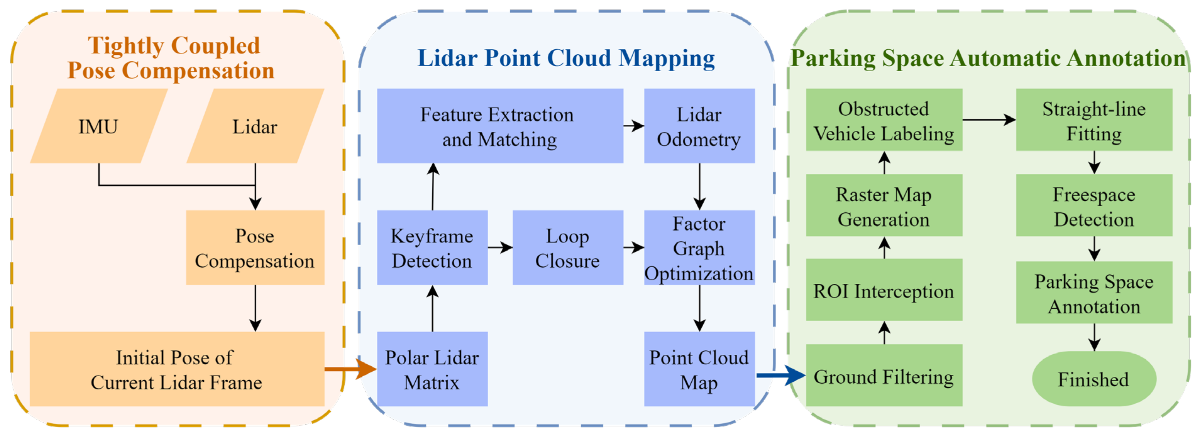
- We propose a parking space detection method based on tightly coupled Lidar and pre-integrated IMU. By integrating Lidar point clouds with IMU data tightly, we construct a high-precision localization and grid map. This method identifies free space between obstacle vehicles using convex hull detection and the Hough transform on the grid map, and finally determines parking spaces based on vehicle size constraints. Therefore, our method achieves high-precision perception of parking scenes.
- We rely solely on Lidar for perceiving the parking scene, eliminating the need for prior maps or parking space information at the input data source. In contrast to current Lidar parking space detection methods that rely on prior information from maps or images, our approach enables precise parking space detection in unknown and complex environments.
- We propose a polarized Lidar matrix transformation method in Lidar SLAM. Our approach converts 3D point clouds into 2D matrices and integrates BEV projections of point cloud grid maps to achieve parking space recognition. By compressing 3D data into 2D, we reduce data storage requirements without sacrificing critical features, thereby addressing the high complexity associated with 3D point cloud processing.
3. Methodology
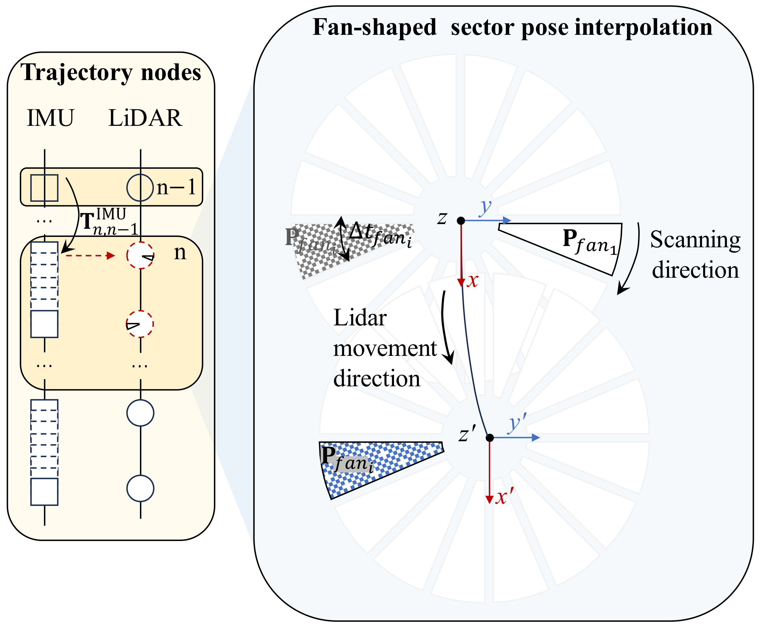
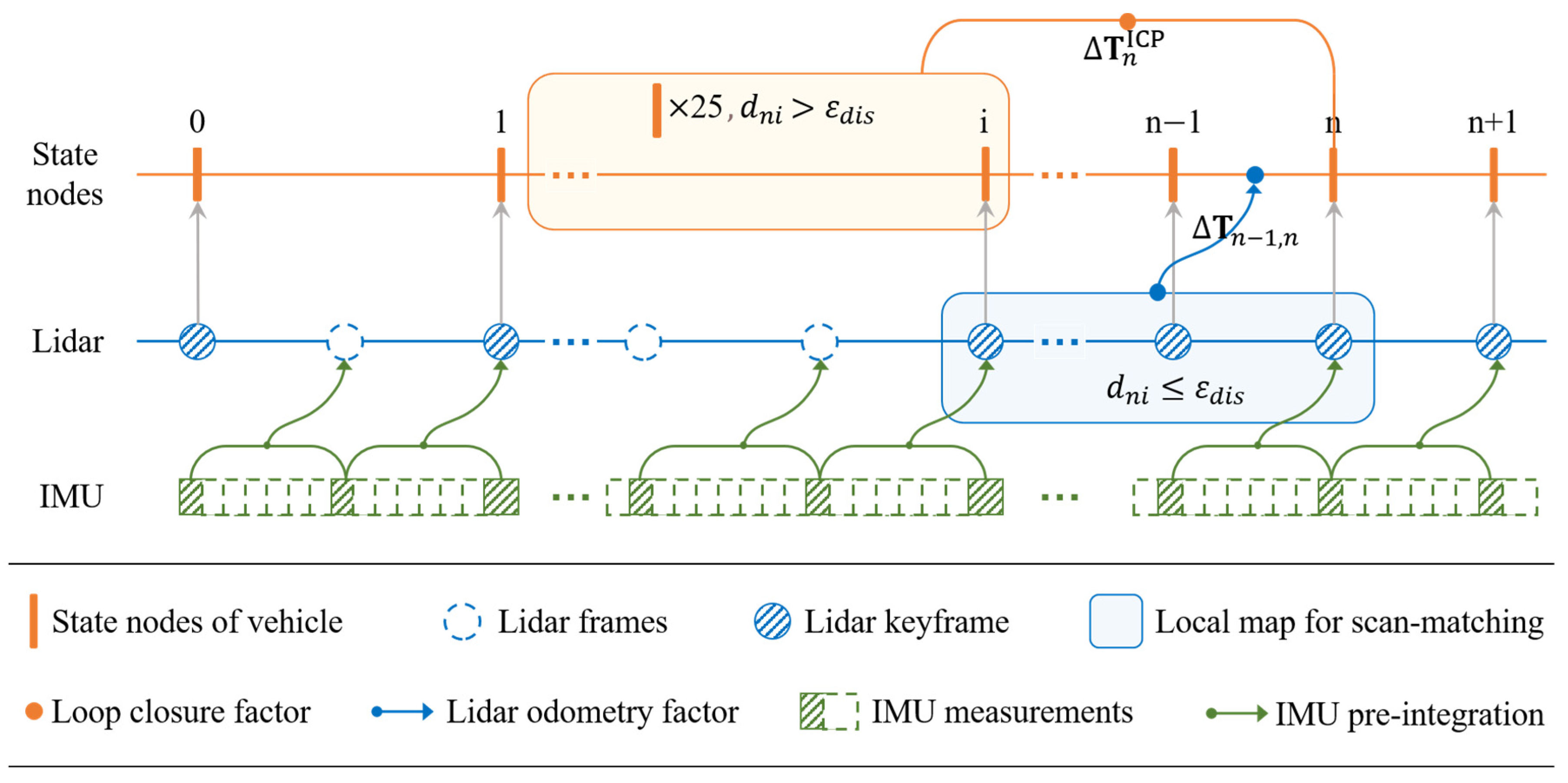
3.1. Tightly Coupled Pose Compensation
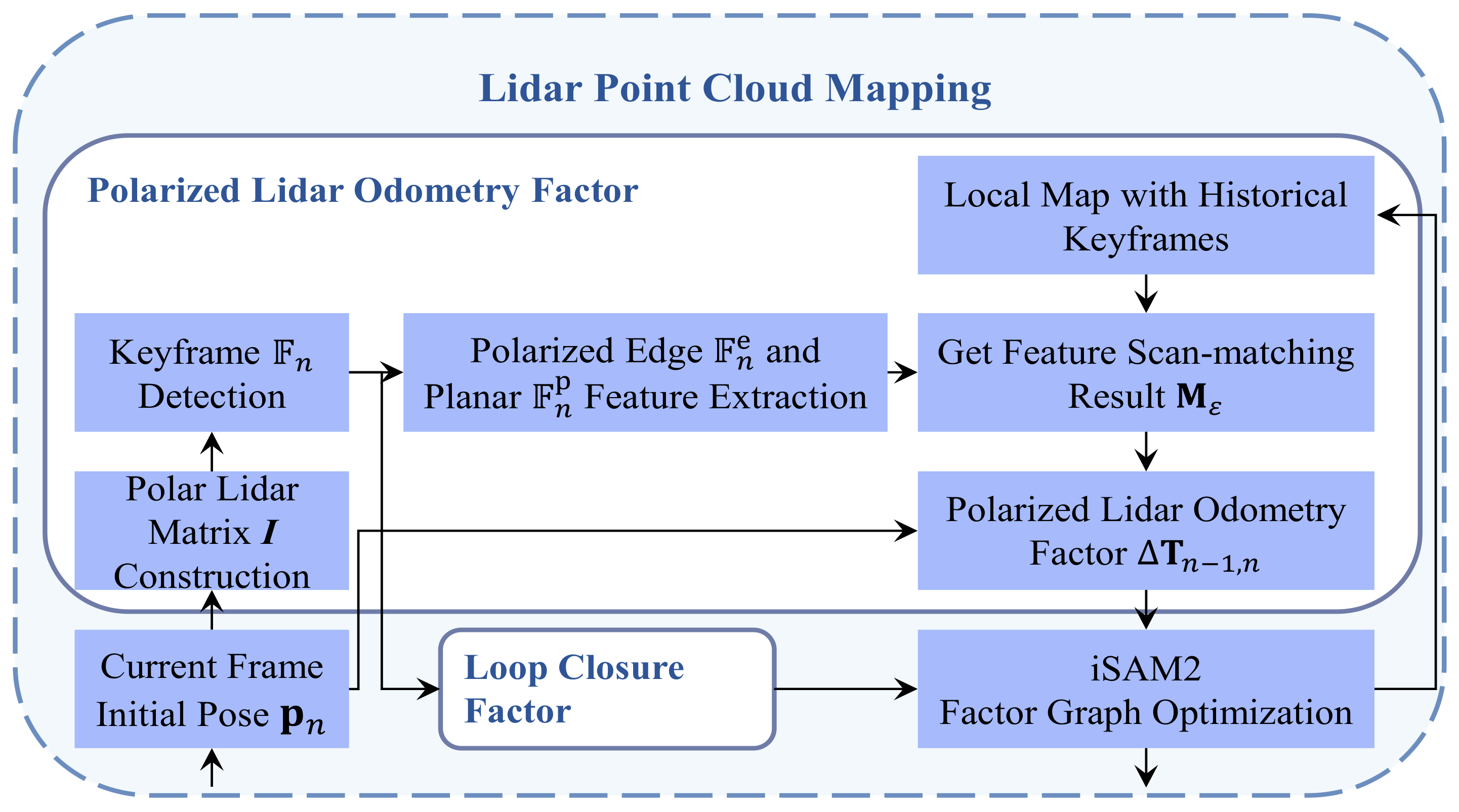
3.2. Lidar Point Cloud Mapping
3.2.1. Polarized Lidar Odometry Factor
- Polar Lidar Matrix Construction
- 2.
- Keyframe Detection
- 3.
- Feature Extraction
- 4.
- Feature scan-matching
3.2.2. Loop Closure Factor
3.3. Parking Space Automatic Annotation
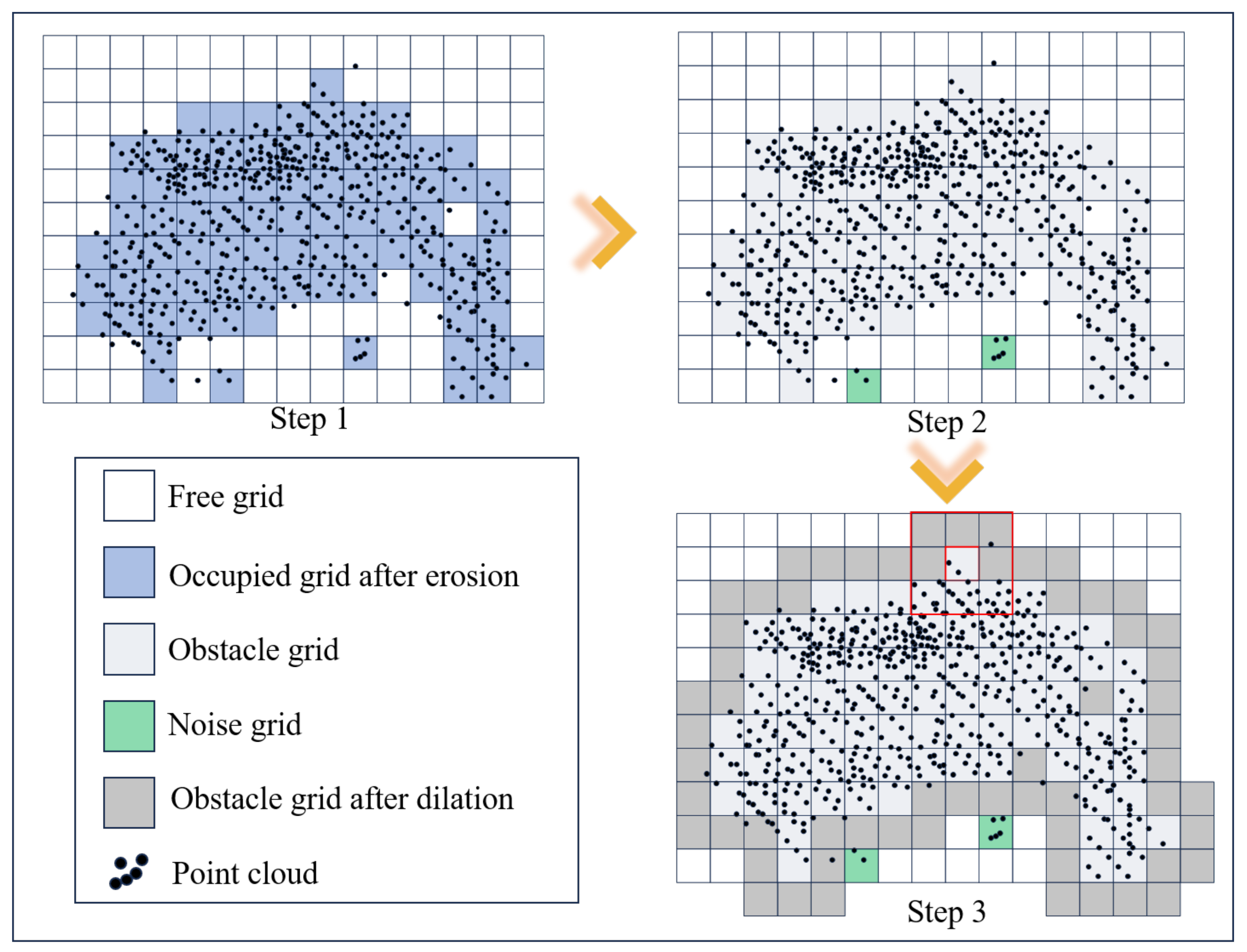
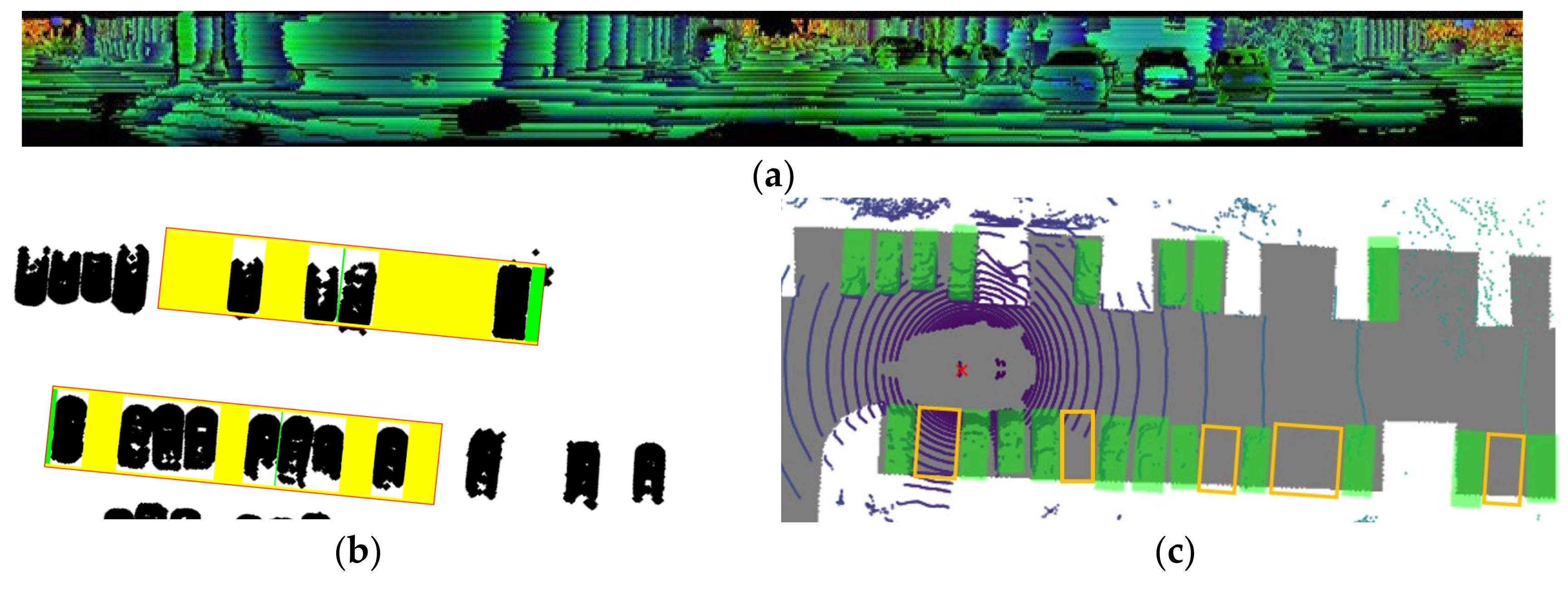
3.3.1. Ground Point Segmentation and Grid Map Construction
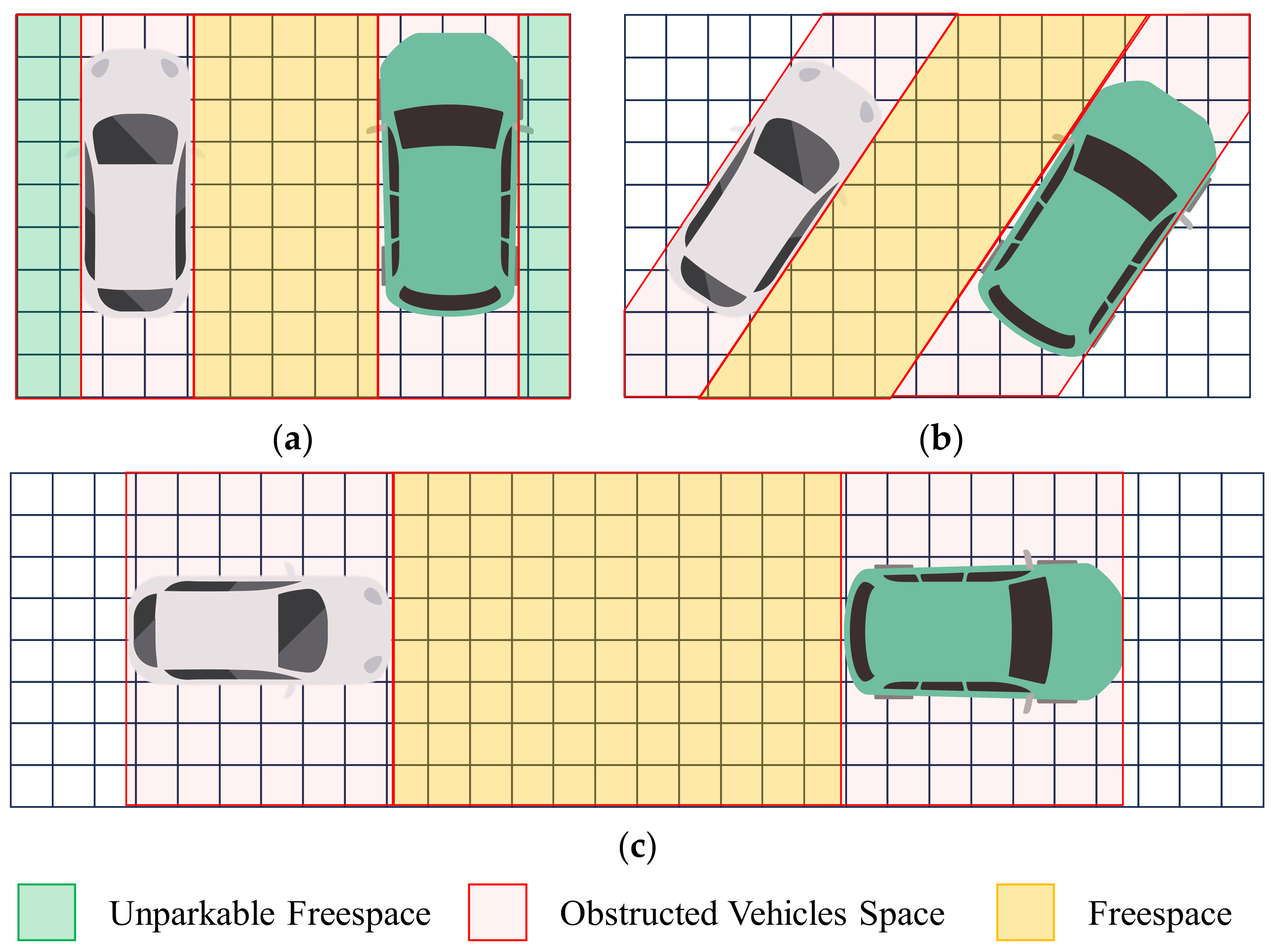
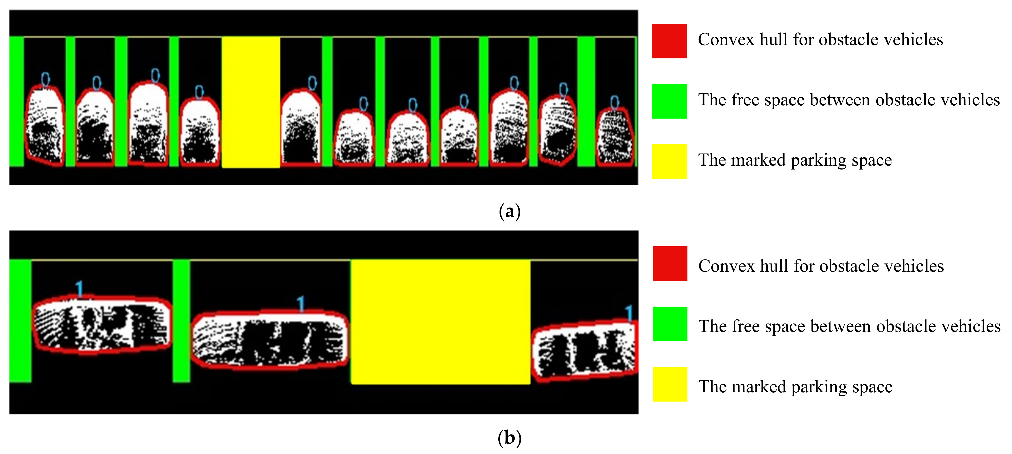
3.3.2. Obstacle Vehicle Detection and Vacancy Annotation
4. Experiments
4.1. Experimental Environments
4.1.1. Local Datasets
4.1.2. Open Datasets
4.2. Performance Evaluation
4.2.1. Verification Experiment
4.2.2. Comparative Experiment
5. Discussion
6. Conclusions
Author Contributions
Funding
Institutional Review Board Statement
Informed Consent Statement
Data Availability Statement
Conflicts of Interest
References
- Yamada, S.; Watanabe, Y.; Kanamori, R.; Sato, K.; Takada, H. Estimation Method of Parking Space Conditions Using Multiple 3D-LiDARs. Int. J. Intell. Transp. Syst. Res. 2022, 20, 422–432. [Google Scholar] [CrossRef]
- Li, F.; Chen, J.; Yuan, Y.; Hu, Z.; Liu, X. Enhanced Berth Mapping and Clothoid Trajectory Prediction Aided Intelligent Underground Localization. Appl. Sci. 2024, 14, 5032. [Google Scholar] [CrossRef]
- Im, G.; Kim, M.; Park, J. Parking Line Based SLAM Approach Using AVM/LiDAR Sensor Fusion for Rapid and Accurate Loop Closing and Parking Space Detection. Sensors 2019, 19, 4811. [Google Scholar] [CrossRef] [PubMed]
- Hasan Yusuf, F.; Mangoud, M.A. Real-Time Car Parking Detection with Deep Learning in Different Lighting Scenarios. Int. J. Comput. Digit. Syst. 2024, 15, 1–9. [Google Scholar] [CrossRef]
- Gkolias, K.; Vlahogianni, E.I. Convolutional Neural Networks for On-Street Parking Space Detection in Urban Networks. IEEE Trans. Intell. Transp. Syst. 2019, 20, 4318–4327. [Google Scholar] [CrossRef]
- Jiang, S.; Jiang, H.; Ma, S.; Jiang, Z. Detection of Parking Slots Based on Mask R-CNN. Appl. Sci. 2020, 10, 4295. [Google Scholar] [CrossRef]
- Ma, Y.; Liu, Y.; Zhang, L.; Cao, Y.; Guo, S.; Li, H. Research Review on Parking Space Detection Method. Symmetry 2021, 13, 128. [Google Scholar] [CrossRef]
- Zainal Abidin, M.; Pulungan, R. A Systematic Review of Machine-Vision-Based Smart Parking Systems. Sci. J. Inform. 2020, 7, 213–227. [Google Scholar] [CrossRef]
- Hwang, J.-H.; Cho, B.; Choi, D.-H. Feature Map Analysis of Neural Networks for the Application of Vacant Parking Slot Detection. Appl. Sci. 2023, 13, 10342. [Google Scholar] [CrossRef]
- Kumar, K.; Singh, V.; Raja, L.; Bhagirath, S.N. A Review of Parking Slot Types and Their Detection Techniques for Smart Cities. Smart Cities 2023, 6, 2639–2660. [Google Scholar] [CrossRef]
- Thakur, N.; Bhattacharjee, E.; Jain, R.; Acharya, B.; Hu, Y.-C. Deep Learning-Based Parking Occupancy Detection Framework Using ResNet and VGG-16. Multimed. Tools Appl. 2024, 83, 1941–1964. [Google Scholar] [CrossRef]
- Luo, Q.; Saigal, R.; Hampshire, R.; Wu, X. A Statistical Method for Parking Spaces Occupancy Detection via Automotive Radars 2016. In Proceedings of the 2017 IEEE 85th Vehicular Technology Conference (VTC Spring), Sydney, NSW, Australia, 4–7 June 2017. [Google Scholar]
- Jiang, H.; Chen, Y.; Shen, Q.; Yin, C.; Cai, J. Semantic Closed-Loop Based Visual Mapping Algorithm for Automated Valet Parking. Proc. Inst. Mech. Eng. Part J. Automob. Eng. 2023, 238, 2091–2104. [Google Scholar] [CrossRef]
- Ye, D.; Yin, X.; Dong, M. Research on Vehicle Parking Aid System Based on Parking Image Enhancement. In Proceedings of the Communications, Signal Processing, and Systems, Online, 18–20 March 2022; Liang, Q., Wang, W., Liu, X., Na, Z., Zhang, B., Eds.; Springer: Singapore, 2022; pp. 192–200. [Google Scholar]
- Fong, W.K.; Mohan, R.; Hurtado, J.V.; Zhou, L.; Caesar, H.; Beijbom, O.; Valada, A. Panoptic nuScenes: A Large-Scale Benchmark for LiDAR Panoptic Segmentation and Tracking. IEEE Robot. Autom. Lett. 2021, 7, 3795–3802. [Google Scholar] [CrossRef]
- Kamiyama, T.; Maeyama, S.; Okawa, K.; Watanabe, K.; Nogami, Y. Recognition of Parking Spaces on Dry and Wet Road Surfaces Using Received Light Intensity of Laser for Ultra Small EVs. In Proceedings of the 2019 IEEE/SICE International Symposium on System Integration (SII), Paris, France, 14–16 January 2019; pp. 494–501. [Google Scholar]
- Gong, Z.; Li, J.; Luo, Z.; Wen, C.; Wang, C.; Zelek, J. Mapping and Semantic Modeling of Underground Parking Lots Using a Backpack LiDAR System. IEEE Trans. Intell. Transp. Syst. 2021, 22, 734–746. [Google Scholar] [CrossRef]
- Jiménez, F.; Clavijo, M.; Cerrato, A. Perception, Positioning and Decision-Making Algorithms Adaptation for an Autonomous Valet Parking System Based on Infrastructure Reference Points Using One Single LiDAR. Sensors 2022, 22, 979. [Google Scholar] [CrossRef] [PubMed]
- Yang, W.; Li, D.; Xu, W.; Zhang, Z. A LiDAR-Based Parking Slots Detection System. Int. J. Automot. Technol. 2024, 25, 331–338. [Google Scholar] [CrossRef]
- Li, L.; Shum, H.P.H.; Breckon, T.P. Less Is More: Reducing Task and Model Complexity for 3D Point Cloud Semantic Segmentation. In Proceedings of the 2023 IEEE/CVF Conference on Computer Vision and Pattern Recognition (CVPR), Vancouver, BC, Canada, 17–24 June 2023; pp. 9361–9371. [Google Scholar]
- Tong, L.; Cheng, L.; Li, M.; Wang, J.; Du, P. Integration of LiDAR Data and Orthophoto for Automatic Extraction of Parking Lot Structure. IEEE J. Sel. Top. Appl. Earth Obs. Remote Sens. 2014, 7, 503–514. [Google Scholar] [CrossRef]
- Zhang, J.; Singh, S. LOAM: Lidar Odometry and Mapping in Real-Time. In Proceedings of the Robotics: Science and Systems X, Robotics: Science and Systems Foundation, Berkeley, CA, USA, 12–16 July 2014. [Google Scholar]
- Rozenberszki, D.; Majdik, A. LOL: Lidar-Only Odometry and Localization in 3D Point Cloud Maps. In Proceedings of the 2020 IEEE International Conference on Robotics and Automation (ICRA), online, 31 May–31 August 2020. [Google Scholar]
- Balazadegan Sarvrood, Y.; Hosseinyalamdary, S.; Gao, Y. Visual-LiDAR Odometry Aided by Reduced IMU. ISPRS Int. J. Geo-Inf. 2016, 5, 3. [Google Scholar] [CrossRef]
- Koide, K.; Yokozuka, M.; Oishi, S.; Banno, A. Globally Consistent and Tightly Coupled 3D LiDAR Inertial Mapping. In Proceedings of the 2022 International Conference on Robotics and Automation (ICRA), Philadelphia, PA, USA, 23–27 May 2022; pp. 5622–5628. [Google Scholar] [CrossRef]
- Liu, Z.; Li, Z.; Liu, A.; Shao, K.; Guo, Q.; Wang, C. LVI-Fusion: A Robust Lidar-Visual-Inertial SLAM Scheme. Remote Sens. 2024, 16, 1524. [Google Scholar] [CrossRef]
- Shan, T.; Englot, B.; Meyers, D.; Wang, W.; Ratti, C.; Rus, D. LIO-SAM: Tightly-Coupled Lidar Inertial Odometry via Smoothing and Mapping. In Proceedings of the 2020 IEEE/RSJ International Conference on Intelligent Robots and Systems (IROS), Las Vegas, NV, USA, 25–29 October 2020; pp. 5135–5142. [Google Scholar]
- Zuo, X.; Geneva, P.; Lee, W.; Liu, Y.; Huang, G. LIC-Fusion: LiDAR-Inertial-Camera Odometry. In Proceedings of the 2019 IEEE/RSJ International Conference on Intelligent Robots and Systems (IROS), Macau, China, 3–8 November 2019; pp. 5848–5854. [Google Scholar] [CrossRef]
- Zhao, S.; Zhang, H.; Wang, P.; Nogueira, L.; Scherer, S. Super Odometry: IMU-Centric LiDAR-Visual-Inertial Estimator for Challenging Environments. In Proceedings of the 2021 IEEE/RSJ International Conference on Intelligent Robots and Systems (IROS), Prague, Czech Republic, 27 September–1 October 2021; pp. 8729–8736. [Google Scholar] [CrossRef]
- Shan, T.; Englot, B.; Ratti, C.; Rus, D. LVI-SAM: Tightly-Coupled Lidar-Visual-Inertial Odometry via Smoothing and Mapping. In Proceedings of the 2021 IEEE International Conference on Robotics and Automation (ICRA), Xi’an, China, 30 May–5 June 2021. [Google Scholar]
- Xu, W.; Zhang, F. FAST-LIO: A Fast, Robust LiDAR-Inertial Odometry Package by Tightly-Coupled Iterated Kalman Filter. IEEE Robot. Autom. Lett. 2021, 6, 3317–3324. [Google Scholar] [CrossRef]
- Zhang, Y. LILO: A Novel Lidar–IMU SLAM System With Loop Optimization. IEEE Trans. Aerosp. Electron. Syst. 2022, 58, 2649–2659. [Google Scholar] [CrossRef]
- Rusinkiewicz, S.; Levoy, M. Efficient Variants of the ICP Algorithm. In Proceedings of the Proceedings Third International Conference on 3-D Digital Imaging and Modeling, Quebec City, QC, Canada, 28 May–1 June 2001; pp. 145–152. [Google Scholar]
- Segal, A.; Haehnel, D.; Thrun, S. Generalized-ICP. In Proceedings of the Robotics: Science and Systems V—Robotics: Science and Systems Foundation, Seattle, WA, USA, 28 June–1 July 2009. [Google Scholar]
- Biber, P.; Strasser, W. The Normal Distributions Transform: A New Approach to Laser Scan Matching. In Proceedings of the Proceedings 2003 IEEE/RSJ International Conference on Intelligent Robots and Systems (IROS 2003) (Cat. No.03CH37453), Las Vegas, NV, USA, 27–31 October 2003; Volume 3, pp. 2743–2748. [Google Scholar]
- Aoki, Y.; Goforth, H.; Srivatsan, R.A.; Lucey, S. PointNetLK: Robust & Efficient Point Cloud Registration Using PointNet. In Proceedings of the IEEE/CVF Conference on Computer Vision and Pattern Recognition (CVPR), Long Beach, CA, USA, 15–20 June 2019. [Google Scholar]
- Yuan, W.; Eckart, B.; Kim, K.; Jampani, V.; Fox, D.; Kautz, J. DeepGMR: Learning Latent Gaussian Mixture Models for Registration. In Proceedings of the Computer Vision–ECCV 2020: 16th European Conference, Glasgow, UK, 23–28 August 2020; Springer International Publishing: Cham, Switzerland, 2020. [Google Scholar]
- Forster, C.; Carlone, L.; Dellaert, F.; Scaramuzza, D. On-Manifold Preintegration for Real-Time Visual–Inertial Odometry. IEEE Trans. Robot. 2017, 33, 1–21. [Google Scholar] [CrossRef]
- Kaess, M.; Johannsson, H.; Roberts, R.; Ila, V.; Leonard, J.J.; Dellaert, F. iSAM2: Incremental Smoothing and Mapping Using the Bayes Tree. Int. J. Robot. Res. 2012, 31, 216–235. [Google Scholar] [CrossRef]
- Zhang, J.; Singh, S. Low-Drift and Real-Time Lidar Odometry and Mapping. Auton. Robots 2017, 41, 401–416. [Google Scholar] [CrossRef]
- Shan, T.; Englot, B. LeGO-LOAM: Lightweight and Ground-Optimized Lidar Odometry and Mapping on Variable Terrain. In Proceedings of the 2018 IEEE/RSJ International Conference on Intelligent Robots and Systems (IROS), Madrid, Spain, 1–5 October 2018; pp. 4758–4765. [Google Scholar]
- Himmelsbach, M.; Hundelshausen, F.V.; Wuensche, H.-J. Fast Segmentation of 3D Point Clouds for Ground Vehicles. In Proceedings of the 2010 IEEE Intelligent Vehicles Symposium, La Jolla, CA, USA, 21–24 June 2010; pp. 560–565. [Google Scholar]
- Yin, T.; Zhou, X.; Krahenbuhl, P. Center-Based 3D Object Detection and Tracking. In Proceedings of the 2021 IEEE/CVF Conference on Computer Vision and Pattern Recognition (CVPR), Nashville, TN, USA, 20–25 June 2021; pp. 11779–11788. [Google Scholar] [CrossRef]
- Zhou, J.; Navarro-Serment, L.E.; Hebert, M. Detection of Parking Spots Using 2D Range Data. In Proceedings of the 2012 15th International IEEE Conference on Intelligent Transportation Systems, Anchorage, AK, USA, 16–19 September 2012; pp. 1280–1287. [Google Scholar]


| Symbols/Variables | Definition |
|---|---|
| The Lidar frame at time , that is, the Lidar frame sequence number. | |
| The Lidar historical key frame number represents the map node number in the mapping, which increases over time. The node number is associated with the vehicle status number. | |
| The pose-transformation matrix from adjacent nodes to is obtained by IMU measurement, . | |
| The time interval between neighboring nodes and . | |
| The point cloud poses of the th laser frame, , represents the coordinate of a point, . | |
| The state of the th laser historical key frame, that is, the th vehicle state node. is the rotation matrix of the pose relative to the origin coordinate, is the translation vector, can represent one another. | |
| The initial value of the th frame pose, and it is calculated based on the pose-transformation matrix provided by the previous node and the IMU. The final pose state of the vehicle after factor graph optimization is . | |
| The fan-shaped sector sequence number in a frame of point cloud data. The fan-shaped sector is divided into equal angles. | |
| The collected pose data of the th fan-shaped sector in the th frame; represents the initial prior pose, and represents the pose after coordinate compensation. | |
| The data-collection time interval between the th fan-shaped sector and the previous. | |
| Represent the rows and columns of the matrix, respectively. represents the matrix values corresponding to the rows and columns of the polarized matrix of point cloud. | |
| The horizontal angular resolution of the Lidar scan. | |
| Angle. represents the horizontal angle of point . represents the vertical angle of point . represents the vertical angle between point and . | |
| The th Lidar historical key frame containing features, the frame coordinates are in the Lidar body coordinate system. , represents the extracted polarized edge feature; represents the extracted polarized planar feature. | |
| The th Lidar historical keyframe in the global coordinate system. | |
| The curvature of the point . | |
| Point sets distributed on the left and right sides of point , represents the number of point sets distributed. | |
| Point depth value. is the depth value of the th point in in the polarized matrix of point cloud, and is the depth value of the th point in in the polarized matrix. | |
| Threshold. represents the curvature threshold for points with edge features; represents the curvature threshold for points with planar features; represents the Euclidean distance threshold; represents the vertical angle difference threshold between point clouds; represents the range threshold for the parallel parking fitting line; represents the range threshold for the perpendicular parking fitting line. | |
| The local map within the range of is composed of historical key frames with edge features and planar features. | |
| Odometry factor for vehicle state to . | |
| Closed-loop detection factor calculated by ICP. | |
| The ROI in the map where parking space detection is required. | |
| Point clouds of different clusters after clustering. represents the category of the point cloud cluster. The number of categories is positively correlated with the number of vehicles contained in the ROI. | |
| Obstacle vehicle point cloud, represents the category of the retained obstacle vehicle. Rules: The sides of the vehicle door are the long side, represented by the character ; the sides of the front and rear windshield of the vehicle are the wide side, represented by the character . | |
| Convex hull point cloud of the obstacle vehicle obtained after drawing the convex hull of the obstacle vehicle. represents different convex hull categories drawn for different obstacle vehicles. | |
| represents the vehicle length size constraint; represents the vehicle width size constraint. |
| Experimental Site | Number of Parking Slots | Type of Parking Slots | ||
|---|---|---|---|---|
| Parallel | Perpendicular | Angled | ||
| Site 1 (2 loops) | 256 | 0 | 185 | 71 |
| Site 2 | 107 | 107 | 0 | 0 |
| Site 3 | 279 | 0 | 279 | 0 |
| Site 4 | 91 | 0 | 91 | 0 |
| Total | 989 | 107 | 740 | 142 |
| Dataset | Device | Beam | S.R. | Resolution | FOV | Range (m) | Acceleration | Angular Rate | ||||
|---|---|---|---|---|---|---|---|---|---|---|---|---|
| Horiz. | Vert. | Horiz. | Vert. | B.S. | S.F. | Bias | S.F. | |||||
| Local | Lidar | 16 | 10 Hz | 0.2° | 2° | 360° | −15° to 15° | 0.5 to 200 | — | — | — | — |
| IMU | — | 100 Hz | — | — | — | — | — | 5 μg | 0.1% | 0.01°/s | 0.1% | |
| Open | Lidar | 32 | 20 Hz | 0.16° | 1.33° | 360° | −30° to 10° | 1 to 70 | — | — | — | — |
| IMU | — | 100 Hz | — | — | — | — | — | 20 μg | 0.06% | 0.2°/s | 0.05% | |
| Experimental Site | Number of Parking Slots | Type of Parking Slots | |
|---|---|---|---|
| Parallel | Perpendicular | ||
| Site 1 (Parking Lot) | 135 | 0 | 135 |
| Site 2 (On-street Parking) | 32 | 32 | 0 |
| Total | 167 | 32 | 135 |
| Test Group | GT | TP | FP | Precision (%) | Recall (%) | F1 Score (%) | |
|---|---|---|---|---|---|---|---|
| Scenario | Site 1 (1st loop) | 256 | 252 | 3 | 98.82 | 98.44 | 98.63 |
| Site 1 (2nd loop) | 256 | 252 | 4 | 98.44 | 98.44 | 98.44 | |
| Site 2 | 107 | 105 | 2 | 98.13 | 98.13 | 98.13 | |
| Site 3 | 279 | 278 | 1 | 99.64 | 99.64 | 99.64 | |
| Site 4 | 91 | 90 | 1 | 98.90 | 98.90 | 98.90 | |
| Type of Parking Slots | Parallel | 107 | 105 | 2 | 98.13 | 98.13 | 98.13 |
| Perpendicular | 740 | 732 | 7 | 99.05 | 98.92 | 98.98 | |
| Angled | 142 | 140 | 2 | 98.59 | 98.59 | 98.59 | |
| Total Number and Average Score | 989 | 977 | 11 | 98.89 | 98.79 | 98.57 | |
| Scenario | Method | GT | TP | FP | Precision (%) | Recall (%) | F1 Score (%) |
|---|---|---|---|---|---|---|---|
| Parking Lot (Perpendicular) | 3D point cloud-based [19] | 135 | 128 | 6 | 95.52 | 94.81 | 95.17 |
| AVM/Lidar fusion-based [3] | 57 | 0 | 100.00 | 42.22 | 59.38 | ||
| The proposed | 135 | 4 | 97.12 | 100.00 | 98.54 | ||
| On-street Parking (Parallel) | 3D point cloud-based [19] | 32 | 31 | 1 | 96.88 | 96.88 | 96.88 |
| AVM/Lidar fusion-based [3] | 14 | 0 | 100.00 | 43.75 | 60.87 | ||
| The proposed | 31 | 1 | 96.88 | 96.88 | 96.88 | ||
| Total Number and Average Score | 3D point cloud-based [19] | 167 | 159 | 7 | 95.78 | 95.21 | 95.50 |
| AVM/Lidar fusion-based [3] | 71 | 0 | 100.00 | 42.51 | 59.66 | ||
| The proposed | 166 | 5 | 97.08 | 99.40 | 98.22 |
| Method | Data Type | Storage (MB) | Runtime Memory (MB) | Runtime (s) | ||||
|---|---|---|---|---|---|---|---|---|
| Input | Output | Input | Output | |||||
| Data | Annotation | Total | ||||||
| 3D Point Cloud-based [19] | 3D Point Cloud | 3D Annotation | 14.16 | 14.16 | 3.10 | 17.26 | 9003.91 (Video Memory) | 3.16 |
| 144.53 | ||||||||
| AVM/Lidar Fusion-based [3] | 6-way Surround View Image | Binary Image | 59.08 | 10.16 | 1.20 | 12.36 | 243.38 | 0.16 |
| 3D Point Cloud | Annotation | 14.16 | 1.00 | |||||
| The Proposed | 3D Point Cloud | Polarized Matrix | 14.16 | 0.65 | 0.03 | 6.38 | 223.40 | 2.95 |
| BEV Annotation | 5.70 | |||||||
Disclaimer/Publisher’s Note: The statements, opinions and data contained in all publications are solely those of the individual author(s) and contributor(s) and not of MDPI and/or the editor(s). MDPI and/or the editor(s) disclaim responsibility for any injury to people or property resulting from any ideas, methods, instructions or products referred to in the content. |
© 2024 by the authors. Licensee MDPI, Basel, Switzerland. This article is an open access article distributed under the terms and conditions of the Creative Commons Attribution (CC BY) license (https://creativecommons.org/licenses/by/4.0/).
Share and Cite
Chen, J.; Li, F.; Liu, X.; Yuan, Y. Robust Parking Space Recognition Approach Based on Tightly Coupled Polarized Lidar and Pre-Integration IMU. Appl. Sci. 2024, 14, 9181. https://doi.org/10.3390/app14209181
Chen J, Li F, Liu X, Yuan Y. Robust Parking Space Recognition Approach Based on Tightly Coupled Polarized Lidar and Pre-Integration IMU. Applied Sciences. 2024; 14(20):9181. https://doi.org/10.3390/app14209181
Chicago/Turabian StyleChen, Jialiang, Fei Li, Xiaohui Liu, and Yuelin Yuan. 2024. "Robust Parking Space Recognition Approach Based on Tightly Coupled Polarized Lidar and Pre-Integration IMU" Applied Sciences 14, no. 20: 9181. https://doi.org/10.3390/app14209181
APA StyleChen, J., Li, F., Liu, X., & Yuan, Y. (2024). Robust Parking Space Recognition Approach Based on Tightly Coupled Polarized Lidar and Pre-Integration IMU. Applied Sciences, 14(20), 9181. https://doi.org/10.3390/app14209181