Abstract
Green’s function plays an important role in the relationship of a future strong earthquake epicenter to the average earthquake potential score. In the frame of the latter, the fractal dimension of the unified scaling law for earthquakes naturally arises. Here it is also shown to be a cornerstone for the development of a new ambient noise tomography methodology, which is applied for example to the west coast of Central Greece. In particular, we show that a fast and reliable 3D shear velocity model extraction is possible without the need for a large amount of data, great-circle propagation assumptions, or the intermediate step of inverting for group velocity maps. The tomography results are consistent with previous studies conducted in the neighboring region.
1. Introduction
The value df ≈ 1.2 describing the fractal dimension of the location of epicenters projected onto the surface of the Earth in a unified scaling law obeyed by the distribution of waiting times between earthquakes (EQs) occurring in California and ranging from tens of seconds to ten years [] can be recovered when considering average EQ potential score (EPS) maps []. Green’s function, which plays an important role in the study of EQs, also arises in the latter study of the average EPS maps [,,].
In particular, we have recently found [] that the epicenter location of a future strong EQ can be estimated by combining a new analysis of seismicity based on a new concept of time termed natural time [,] with EQ networks based on similar activity patterns [] and EQ nowcasting [,,,,,,,]. This is based on the construction of average EPS maps. Specifically, the two-dimensional Green’s function has been recovered when studying the interrelation of a future strong EQ epicenter with the average EPS.
Traditionally, seismologists analyze distinct seismic phases (e.g., P, S, surface waves) that travel through the Earth to draw conclusions about the Earth’s interior structure and properties. According to Larose [], a daily seismic record is composed of the following: 95% of ambient seismic noise, 4% of coda waves, and 1% related to body waves from earthquakes or explosions. Ambient noise consists of continuous vibrations triggered by low-amplitude sources, such as microtremors.
In broad terms, the higher frequency noise (exceeding 1 Hz) primarily stems from human activities, such as transportation and industrial operations. Conversely, noise below 1 Hz, called microseismic noise, refers to the interaction of natural elements like wind, storms, and oceanic waves with the solid Earth. Since these waves travel through the Earth, they ought to carry information about the medium through which they travel [,]. The pioneering work of Aki [] and Claerbout [] helped develop the technique for seismic applications and provided the framework upon which modern theory is based. A signal at seismic station A can be cross-correlated with a signal at seismic station B to reproduce a virtual source–receiver pair. It has been shown in various theoretical studies [] that this cross-correlation can reproduce the surface waves of the Earth’s impulse response—or the Green’s function—as if triggered by a point source. The experimental results of Campillo and Paul [], which verified the validity of this methodology by extracting the surface wave Green’s functions between pairs of seismic stations in Mexico with the cross-correlation of coda waves, are considered a milestone in the field of ambient noise methods. By measuring the dispersion relation of these surface waves between multiple pairs of stations, surface wave tomography is possible [].
Below, a new ambient noise tomography (ANT) methodology will be presented. As an example, it will be applied to the area of western Greece depicted in Figure 1, namely the region enclosed by the stations shown at latitudes 38–39° N and longitudes 20–22° E, to derive a reliable 3D shear wave speed model.
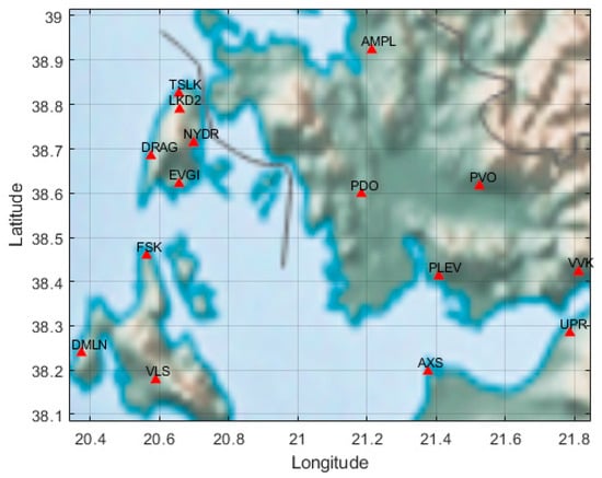
Figure 1.
The area of interest along with the Hellenic Unified Seismological Network (HUSN) stations denoted with red triangles.
2. Materials and Methods
The data consist of 10 days (9 October 2021–19 October 2021) of continuous seismogram recordings from 15 seismic stations of the Hellenic Unified Seismological Network (HUSN), which were retrieved using the ObsPy framework []. Any gaps in these measurements were replaced with zeros. The Z components were used in this analysis to obtain Rayleigh waves. We applied the following standard preprocessing steps [], which were implemented asynchronously while retrieving the data: First, the waveforms were decimated from 100 to 10 Hz, tapered, demeaned, and detrended by subtracting a third-order spline with 500 samples between the spline nodes. Later, the instrument response was removed, after applying a band-pass filter with corner frequencies 0.05, 0.1, 4, 4.5 Hz, and a 1-bit amplitude normalization procedure, under which we applied the sign function to the signal. According to Nahakara [], the derivative of the cross-correlation is as follows:
Between the recordings, a and b of the two stations can be related to the Green’s function between them. Namely, this is found as follows, with ∗ denoting convolution:
By the convolution theorem, assuming the autocorrelation is a delta-like function, with A, B denoting the Fourier transforms of the recordings a, b and being the complex conjugate of A, this is equivalent to the following:
3. Results and Discussion
3.1. Experimental Green’s Functions (EGFs)
Multiplication in the frequency domain, along with the use of thread-based parallelism, allows for the rapid calculation of EGFs between pairs of stations. Two quality control measures were taken to accept or reject a potential EGF between pairs of stations. Firstly, a signal-to-noise ratio (SNR) threshold of 8 was used, where SNR is defined as the ratio of the maximum absolute value of the signal (from −80 s to 80 s time lag) to the standard deviation of a noisy signal window (from 100 s to 200 s time lag). Secondly, each EGF group should be in the range of 1.8–5.5 km/s. The envelope was calculated as the absolute value of the analytic signal, i.e., its Hilbert Transform. The EGFs obtained are presented in Figure 2. It is worth noting that no stacking was used, since both the pre-processing and the cross-correlation was applied to the full 10 days of recording of each station. From a total of 0.5 × n(n − 1) = 105 (for n = 15) cross-correlations, 40 were rejected.
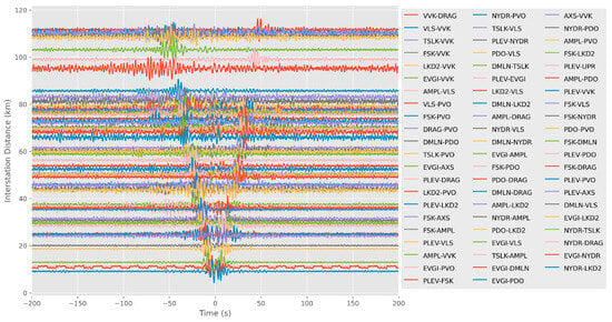
Figure 2.
The normalized EGF for each pair of stations, plotted in increasing interstation distance with respect to time.
3.2. Frequency Time Analysis (FTAN) and 1D Inversion
After the extraction of each EGF, FTAN [] was applied to obtain the group velocity as a function of the period, using the EGFAnalysisTimeFreq dispersion software []. The group velocity dispersion analysis uses a Gaussian window G in the frequency domain, which is applied as a narrow band-pass filter at each central frequency. Considering f as the frequency, fc as the central frequency, and A as an interstation-distance-dependent coefficient, where A is equal to 5 for interstation distances less than 100 km and A is equal to 8 otherwise, we obtain the following:
To obtain reliable dispersion measurements, we accept a frequency-dependent velocity of the fundamental mode, provided that its SNR is at least 5 and its ratio of the interstation distance over its wavelength is at least 2 []. Here, the SNR is frequency-dependent and for each central frequency, it is equal to the maximum amplitude of the envelope in the signal window divided by the mean amplitude of the envelope of the 150 s long noise window right after the signal window. The signal window is such that the group velocity lies between 1.8 and 5.5 km/s, according to the interstation distance. The period range under investigation is between 1 and 10 s, after examining the peak of the probabilistic power spectral densities of several stations for the given time frame. An example of such a measurement for a pair of stations is shown in Figure 3. All dispersion curves were later averaged for periods between 1 and 8 s and the average was smoothed by applying a moving mean scheme (Figure 4).
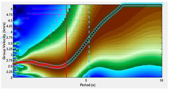
Figure 3.
A selected group velocity curve of the fundamental mode for the EVGI-LKD2 station pair. Only the red circles to the left of the vertical red line are considered valid measurements, as only those points satisfy the condition that the interstation distance over wavelength ratio is larger than 2. Similarly, the dashed cyan line is drawn when such a ratio becomes equal to 3. Brown colors indicate high amplitudes, while blue colors denote low amplitudes.
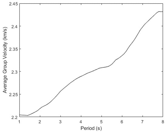
Figure 4.
Average group velocity dispersion curve, for periods between 1 and 8 s, smoothed by applying a 15-point moving average.
In general, the effect of a water layer can make it difficult to measure unambiguously the fundamental-mode dispersion velocities at frequencies above 0.1 Hz []. However, since here this is not the case (Figure 3), we assume the effect of the water layer to be minimal, due to its small depth which is at most 400 m in the study area [].
To assess which 1D shear velocity model best fits the average dispersion curve (Figure 4), we applied a Neighborhood Algorithm [] as an inversion technique, using the software Geopsy v3.4.2 []. This technique improves upon the efficiency of a standard Monte Carlo method by introducing a sampling preference over the more promising—based on the results obtained so far—subsets of the parameter space []. The forward problem solution [] is based on the theoretical elastic computation of a dispersion curve for a stack of horizontal and homogeneous layers [,,,]. The initial model consists of four layers from the surface up to infinite depth with increasing velocity, Vp from 0.2 to 5 km/s, Vs from 0.5 to 3.5 km/s, and Poisson’s ratio from 0.25 to 0.5 to cover all possible solutions. A constant density of 2000 kg/m3 was chosen, due to the fact that the study area mainly consists of sediments and limestones [], which indicate a density range typically between 1600 and 2750 kg/m3 [].
3.3. Inversion for a 3D Vs Model and Discussion
To invert the Rayleigh wave group velocity data to obtain 3D shear velocity models, we applied the algorithm proposed by Fang et al. []. This algorithm does not make the inherent assumption of straight ray propagation which is commonly used in most ANT studies, but instead solves the eikonal equation with the fast-marching method [] at each period, to reproduce a more appropriate ray path between source and receiver. This algorithm avoids the intermediate step of inversion for the group velocity map. The initial solution proposed (along with the depth constraint associated with it) was the 1D Vs profile in Figure 5.
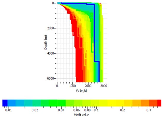
Figure 5.
The 1D Vs model obtained in this study by applying the Neighborhood Algorithm. Note that the deviation of the best model (blue line) from the true model is of the order of 10−3. The misfit value for each candidate model is defined as where is the data group velocity at frequency , is the candidate model’s group velocity at frequency , and n is the number of frequency samples considered []. Here, n is 71.
We have assessed the validity of the inversion algorithm by performing a checkerboard test, in which the synthetic travel time data produced by the checkerboard model are inverted (after adding 2% Gaussian noise). The checkerboard model (Figure 6a) is produced by the spatially symmetric perturbation of our initial solution and shows a good correspondence with the model produced by the inversion of the synthetic data (Figure 6b), inside the area covered by the stations. The value λ = 4 was chosen as the value of the Lagrange multiplier of the inversion algorithm, as it produced the best result during the checkerboard test compared to lower values (i.e., with less smoothing).
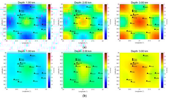
Figure 6.
(a) Horizontal slices of the original checkerboard model and (b) horizontal slices of the inverted synthetic travel times, which are produced from the checkerboard model.
The iteratively reweighted least squares method was applied until convergence, at which point the objective function was close to zero, and the final model produced is shown in Figure 7. Four layers are assumed (their number is a priori determined during parameterization) with increasing velocity from 1.7 ± 0.3 km/s at the surface up to 2.8 ± 0.2 km/s at 4.5 km depth. During the inversion process the wave speed was constrained between 1 and 3 km/s. Our results are consistent with previous studies in northern and eastern neighboring regions [,]. Considering the known geology derived from borehole data in neighboring regions, which showed that approximately for the first half-kilometer there are Neogene sediments while the Vigla and Pantokrator Limestones extend below [], the final 3D model, and known shear velocity–soil type relations (i.e., in brief, that the value of Vs below 2 km/s corresponds to sediments while the value above it corresponds to sound limestones []), we infer the existence of loose sedimentary rocks until a depth of 500 m, while below we infer the existence of limestones. The curvature of the layers lies outside the area covered by the stations, so it is not considered.

Figure 7.
(a) Two cross-sections of the 3D shear velocity (final) model found in this study. One is of constant latitude at 38.4° N and the other is of constant longitude at 21° E. (b) Shear velocity contours at 0, 2, and 4 km depth.
The uncertainty of the final model is determined by the application of a Monte Carlo error propagation technique []. After producing synthetic travel times from the final model, we inverted them (after adding 2% Gaussian noise) many times and measured the standard deviation of the resultant set of models (Figure 8). Inside the area defined by the outermost stations, the uncertainty of the wave speed model is small (≈±0.2 km/s).

Figure 8.
Horizontal slices of the standard deviation measured from the set of models produced by the inversion of the synthetic travel times. The latter are derived by solving the forward problem, assuming the final model shown in Figure 7 is valid.
To further investigate if the model is well constrained in terms of depth, we calculated using disba [] the sensitivity of the surface wave group velocity to the shear wave speed for different periods, from the final 1D model (Figure 9a). The latter was calculated from the mean and standard deviation of different horizontal slices of the final 3D model, including only data inside the area defined by the seismic stations. Apart from the final 1D model, the corresponding compressional wave speed and density profile were also required. We assumed a constant density of 2.000 kg/m3 and a Vp/Vs ratio of 2. As expected, the larger periods are more sensitive to larger depths. A similar conclusion can be reached by running a checkerboard test for the same distinct periods, where the central wave speed anomaly in the study area is more adequately recovered with increasing periods at larger depths (Figure 10).
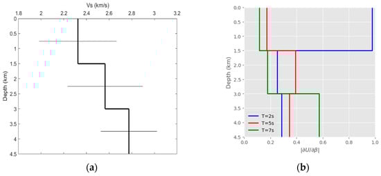
Figure 9.
(b) The normalized sensitivity of the group velocity to shear velocity for different periods, derived from (a) the final 1D model, whose error bars denote standard deviation.
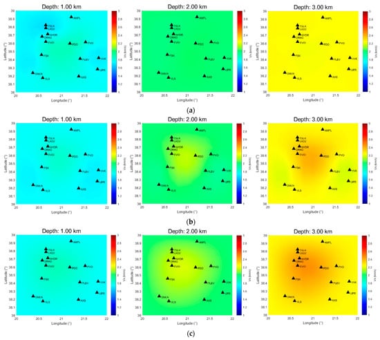
Figure 10.
Horizontal slices of the inverted checkerboard model of Figure 6a at different periods. (a) T = 2 s, (b) T = 5 s, (c) T = 7 s.
4. Discussion and Conclusions
The present methodology shows promising and reasonable results without the need for large amounts of data, with low runtime speeds, and without the assumption of great-circle propagation or the necessity of inversion for group velocity maps. A comparison of our methodology with more commonly applied ANT methods is shown in Figure 11. Initially, the seismic data retrieval is intermingled with their preprocessing by applying multi-threading programming, which reduces runtime speeds compared to synchronous programming. Moreover, splits and stacks of the data are avoided and the cross-correlations are not performed in the time domain; instead, the whole data series of each station is cross-correlated with each other in the frequency domain. In addition, instead of implementing a 2D inversion for each frequency to derive group velocity maps, a process where straight-ray propagation is traditionally assumed [], a single 1D inversion of the mean group dispersion curve is obtained. Finally, instead of deriving the 3D model as a composite of many 1D inversions, a direct surface wave inversion method is performed where the sensitivity kernels and ray-paths are iteratively updated until convergence. As far as the new ambient noise tomography methodology is concerned, the following conclusions apply: By cross-correlating in the frequency domain a few days of vertical component noise recordings for each pair of stations on the west coast of central Greece, we extracted the EGFs, as if one station were the source and the other the receiver. Subsequently, applying FTAN, we inferred the group dispersion relation for each Rayleigh fundamental mode. The average of these dispersion relations was then inverted for a 1D shear wave velocity model, which was later proposed as the initial solution in the 3D inversion process. The 3D Vs model produced was consistent with previous studies conducted in neighboring areas.
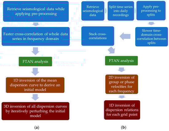
Figure 11.
Flowchart for (a) the methodology applied in this study and (b) the common methodology applied in ANT.
Author Contributions
Conceptualization, P.K.V.; methodology, P.K.V. and N.V.S.; software, P.K.V.; validation, P.K.V. and N.V.S.; formal analysis, P.K.V.; investigation, P.K.V. and N.V.S.; resources, P.K.V.; data curation, P.K.V.; writing—original draft preparation, P.K.V. and N.V.S.; writing—review and editing, P.K.V. and N.V.S.; visualization, P.K.V.; supervision, P.K.V. and N.V.S.; project administration, P.K.V. All authors have read and agreed to the published version of the manuscript.
Funding
This research received no external funding.
Institutional Review Board Statement
Not applicable.
Informed Consent Statement
Not applicable.
Data Availability Statement
The data used in this study are publicly available at https://www.fdsn.org/webservices/datacenters/, accessed on 28 August 2023.
Conflicts of Interest
The authors declare no conflicts of interest.
References
- Bak, P.; Christensen, K.; Danon, L.; Scanlon, T. Unified Scaling Law for Earthquakes. Phys. Rev. Lett. 2002, 88, 178501. [Google Scholar] [CrossRef] [PubMed]
- Varotsos, P.K.; Perez-Oregon, J.; Skordas, E.S.; Sarlis, N.V. Estimating the Epicenter of an Impending Strong Earthquake by Combining the Seismicity Order Parameter Variability Analysis with Earthquake Networks and Nowcasting: Application in Eastern Mediterranean. Appl. Sci. 2021, 11, 10093. [Google Scholar] [CrossRef]
- Perez-Oregon, J.; Varotsos, P.K.; Skordas, E.S.; Sarlis, N.V. Estimating the Epicenter of a Future Strong Earthquake in Southern California, Mexico, and Central America by Means of Natural Time Analysis and Earthquake Nowcasting. Entropy 2021, 23, 1658. [Google Scholar] [CrossRef] [PubMed]
- Christopoulos, S.-R.G.; Varotsos, P.K.; Perez-Oregon, J.; Papadopoulou, K.A.; Skordas, E.S.; Sarlis, N.V. Natural Time Analysis of Global Seismicity. Appl. Sci. 2022, 12, 7496. [Google Scholar] [CrossRef]
- Varotsos, P.A.; Sarlis, N.V.; Skordas, E.S. Long-Range Correlations in the Electric Signals That Precede Rupture. Phys. Rev. E 2002, 66, 011902. [Google Scholar] [CrossRef]
- Varotsos, P.A.; Sarlis, N.V.; Skordas, E.S. Natural Time Analysis: The New View of Time. Part II. Advances in Disaster Predictions Using Complex Systems; Springer Nature: Cham, Switzerland, 2023. [Google Scholar] [CrossRef]
- Tenenbaum, J.N.; Havlin, S.; Stanley, H.E. Earthquake Networks Based on Similar Activity Patterns. Phys. Rev. E 2012, 86, 046107. [Google Scholar] [CrossRef]
- Luginbuhl, M.; Rundle, J.B.; Turcotte, D.L. Natural time and nowcasting induced seismicity at the Groningen gas field in the Netherlands. Geophys. J. Int. 2018, 215, 753–759. [Google Scholar] [CrossRef]
- Luginbuhl, M.; Rundle, J.B.; Hawkins, A.; Turcotte, D.L. Nowcasting earthquakes: A comparison of induced earthquakes in Oklahoma and at the Geysers, California. Pure Appl. Geophys. 2018, 175, 49–65. [Google Scholar] [CrossRef]
- Rundle, J.B.; Turcotte, D.L.; Donnellan, A.; Grant Ludwig, L.; Luginbuhl, M.; Gong, G. Nowcasting Earthquakes. Earth Space Sci. 2016, 3, 480–486. [Google Scholar] [CrossRef]
- Rundle, J.B.; Luginbuhl, M.; Giguere, A.; Turcotte, D.L. Natural Time, Nowcasting and the Physics of Earthquakes: Estimation of Seismic Risk to Global Megacities. Pure Appl. Geophys. 2018, 175, 647–660. [Google Scholar] [CrossRef]
- Rundle, J.B.; Giguere, A.; Turcotte, D.L.; Crutchfield, J.P.; Donnellan, A. Global Seismic Nowcasting with Shannon Information Entropy. Earth Space Sci. 2019, 6, 191–197. [Google Scholar] [CrossRef]
- Rundle, J.B.; Donnellan, A. Nowcasting Earthquakes in Southern California with Machine Learning: Bursts, Swarms, and Aftershocks May Be Related to Levels of Regional Tectonic Stress. Earth Space Sci. 2020, 7, e2020EA001097. [Google Scholar] [CrossRef]
- Rundle, J.; Stein, S.; Donnellan, A.; Turcotte, D.L.; Klein, W.; Saylor, C. The Complex Dynamics of Earthquake Fault Systems: New Approaches to Forecasting and Nowcasting of Earthquakes. Rep. Prog. Phys. 2021, 84, 076801. [Google Scholar] [CrossRef] [PubMed]
- Rundle, J.B.; Donnellan, A.; Fox, G.; Crutchfield, J.P. Nowcasting Earthquakes by Visualizing the Earthquake Cycle with Machine Learning: A Comparison of Two Methods. Surv. Geophys. 2022, 43, 483–501. [Google Scholar] [CrossRef]
- Larose, É. Mesoscopics of ultrasound and seismic waves: Application to passive imaging. Ann. Phys. 2006, 31, 1–126. [Google Scholar] [CrossRef]
- Shapiro, N.M.; Campillo, M.; Singh, S.K.; Pacheco, J. Seismic channel waves in the accretionary prism of the Middle America Trench. Geophys. Res. Lett. 1998, 25, 101–104. [Google Scholar] [CrossRef]
- Snieder, R.; Wapenaar, K. Imaging with ambient noise. Phys. Today 2010, 63, 44–49. [Google Scholar] [CrossRef]
- Aki, K. Space and time spectra of stationary stochastic waves, with special reference to microtremors. Bull. Earthq. Res. Inst. 1957, 35, 415–457. [Google Scholar] [CrossRef]
- Claerbout, J.F. Synthesis of a Layered Medium from ITS Acoustic Transmission Response. Geophysics 1968, 33, 264–269. [Google Scholar] [CrossRef]
- Campillo, M.; Paul, A. Long-Range Correlations in the Diffuse Seismic Coda. Science 2003, 299, 547–549. [Google Scholar] [CrossRef]
- Shapiro, N.M.; Campillo, M.; Stehly, L.; Ritzwoller, M.H. High-resolution surface-wave tomography from ambient seismic noise. Science 2005, 307, 1615–1618. [Google Scholar] [CrossRef] [PubMed]
- Beyreuther, M.; Barsch, R.; Krischer, L.; Megies, T.; Behr, Y.; Wassermann, J. ObsPy: A Python Toolbox for Seismology. Seismol. Res. Lett. 2010, 81, 530–533. [Google Scholar] [CrossRef]
- Bensen, G.D.; Ritzwoller, M.H.; Barmin, M.P.; Levshin, A.L.; Lin, F.; Moschetti, M.P.; Shapiro, N.M.; Yang, Y. Processing seismic ambient noise data to obtain reliable broad-band surface wave dispersion measurements. Geophys. J. Int. 2007, 169, 1239–1260. [Google Scholar] [CrossRef]
- Nahakara, H. A systematic study of theoretical relations between spatial correlation and Green’s function in one-, two- and three-dimensional random scalar wavefields. Geophys. J. Int. 2006, 167, 1097–1105. [Google Scholar] [CrossRef]
- Dziewonski, A.M.; Block, S.; Landisman, M. A technique for the analysis of transient seismic signals. Bull. Seism. Soc. Am. 1969, 59, 427–444. [Google Scholar] [CrossRef]
- Yao, H. Github. 2023. Available online: https://github.com/ShaoboYang-USTC/EGFAnalysisTimeFreq (accessed on 12 September 2023).
- Carvalho, J.; Silveira, G.; Kiselev, S.; Custódio, S.; Ramalho, R.S.; Stutzmann, E.; Schimmel, M. Crustal and uppermost mantle structure of Cape Verde from ambient noise tomography. Geophys. J. Int. 2022, 231, 1421–1433. [Google Scholar] [CrossRef]
- Le Pichon, X.; Lallemant, S.J.; Chamot-Rooke, N.; Lemeur, D.; Pascal, G. The Mediterranean Ridge backstop and the Hellenic nappes. Mar. Geol. 2002, 186, 111–125. [Google Scholar] [CrossRef]
- Sambridge, M. Geophysical inversion with a neighbourhood algorithm: I. Searching a parameter space. Geophys. J. Int. 1999, 138, 479–494. [Google Scholar] [CrossRef]
- Wathelet, M.; Chatelain, J.-L.; Cornou, C.; Di Giulio, G.; Guillier, B.; Ohrnberger, M.; Savvaidis, A. Geopsy: A User-Friendly Open-Source Tool Set for Ambient Vibration Processing. Seismol. Res. Lett. 2020, 91, 1878–1889. [Google Scholar] [CrossRef]
- Wathelet, M. An improved neighborhood algorithm: Parameter conditions and dynamic scaling. Geophys. Res. Lett. 2008, 35, L09301. [Google Scholar] [CrossRef]
- Wathelet, M.; Jongmans, D.; Ohrnberger, M. Surface wave inversion using a direct search algorithm and its application to ambient vibration measurements. Near Surf. Geophys. 2004, 2, 211–221. [Google Scholar] [CrossRef]
- Thomson, W.T. Transmission of elastic waves through a stratified solid medium. J. Appl. Phys. 1950, 21, 89–93. [Google Scholar] [CrossRef]
- Haskell, N.A. The dispersion of surface waves on a multi-layered medium. Bull. Seismol. Soc. Am. 1953, 43, 17–34. [Google Scholar] [CrossRef]
- Knopoff, L. A matrix method for elastic wave problems. Bull. Seismol. Soc. Am. 1964, 54, 431–438. [Google Scholar] [CrossRef]
- Dunkin, J.W. Computation of modal solutions in layered, elastic media at high frequencies. Bull. Seismol. Soc. Am. 1965, 55, 335–358. [Google Scholar] [CrossRef]
- Karakitsios, V. The Influence of Preexisting Structure and Halokinesis on Organic Matter Preservation and Thrust System Evolution in the Ionian Basin, Northwest Greece. AAPG Bull. 1995, 79, 960–980. [Google Scholar] [CrossRef]
- Sharma, P.V. Environmental and Engineering Geophysics; Cambridge University Press: Cambridge, UK, 1997. [Google Scholar] [CrossRef]
- Fang, H.; Yao, H.; Zhang, H.; Huang, Y.C.; van der Hilst, R.D. Direct inversion of surface wave dispersion for three-dimensional shallow crustal structure based on ray tracing: Methodology and application. Geophys. J. Int. 2015, 201, 1251–1263. [Google Scholar] [CrossRef]
- Rawlinson, N.; Sambridge, M. Wave front evolution in strongly heterogeneous layered media using the fast marching method. Geophys. J. Int. 2004, 156, 631–647. [Google Scholar] [CrossRef]
- Haslinger, F.; Kissling, E.; Ansorge, J.; Hatzfeld, D.; Papadimitriou, E.; Karakostas, V.; Makropoulos, K.; Kahle, H.-G.; Peter, Y. 3D crustal structure from local earthquake tomography around the Gulf of Arta (Ionian region, NW Greece). Tectonophysics 1999, 304, 201–218. [Google Scholar] [CrossRef]
- Giannopoulos, D.; Rivet, D.; Sokos, E.; Deschamps, A.; Mordret, A.; Lyon-Caen, H.; Bernard, P.; Paraskevopoulos, P.; Tselentis, A. Ambient noise tomography of the western Corinth Rift, Greece. Geophys. J. Int. 2017, 211, 284–299. [Google Scholar] [CrossRef]
- Jia, J. Soil Dynamics and Foundation Modeling; Springer: Cham, Switzerland, 2018. [Google Scholar] [CrossRef]
- Aster, R.C.; Borchers, B.; Thurber, C.H. Parameter Estimation and Inverse Problems, 3rd ed.; Elsevier: Amsterdam, The Netherlands, 2019. [Google Scholar] [CrossRef]
- Luu, K. Disba: Numba-Accelerated Computation of Surface Wave Dispersion. v0.6.1; Zenodo: Geneva, Switzerland, 2021. [Google Scholar] [CrossRef]
- Barmin, M.P.; Ritzwoller, M.; Levshin, A. A Fast and Reliable Method for Surface Wave Tomography. Pure Appl. Geophys. 2001, 158, 1351–1375. [Google Scholar] [CrossRef]
Disclaimer/Publisher’s Note: The statements, opinions and data contained in all publications are solely those of the individual author(s) and contributor(s) and not of MDPI and/or the editor(s). MDPI and/or the editor(s) disclaim responsibility for any injury to people or property resulting from any ideas, methods, instructions or products referred to in the content. |
© 2024 by the authors. Licensee MDPI, Basel, Switzerland. This article is an open access article distributed under the terms and conditions of the Creative Commons Attribution (CC BY) license (https://creativecommons.org/licenses/by/4.0/).