An Improved Empirical Wavelet Transform Filtering Method for Rail-Head Surface-Defect Magnetic-Flux Leakage Signal

Abstract

The rail is an important factor in railway traffic safety. Surface defects in the rail head comprise a common type of rail damage, and magnetic flux leakage (MFL) technology is applied for its detection. MFL detection is influenced by various factors, resulting in high noise and a low signal-to-noise ratio (SNR) in the collected MFL signal, which influence defect assessment. This article improves the empirical wavelet transform (EWT) to apply it to rail surface-defect MFL signal filtering. A boundary optimization method based on mutual information (MI) is proposed to reduce the boundary redundancy caused by adaptive spectrum division. A method for component selection based on MI and kurtosis is proposed to select the suitable components from the decomposed components for signal reconstruction. The experimental results show that the method can effectively filter out the interference in the MFL signal, and the effectiveness is superior to the traditional methods, such as complementary ensemble empirical mode decomposition (CEEMD) and wavelet transform (WT).

1. Introduction

As an important component of railway tracks, the rail withstands long-term pressure from train wheelsets and external environmental effects, leading to problems such as defects and material degradation, causing safety hazards for railway transportation [1]. The timely and efficient detection of early minor defects in the rail surface is of great significance for improving safety and preventing accidents in railway transportation.

Due to advantages such a high detection sensitivity, simple detection device structure, rapid detection speed, and non-contact detection, magnetic flux leakage (MFL) detection is frequently used for the non-destructive detection of surface defects in ferromagnetic materials, such as rails and steel pipes [2].

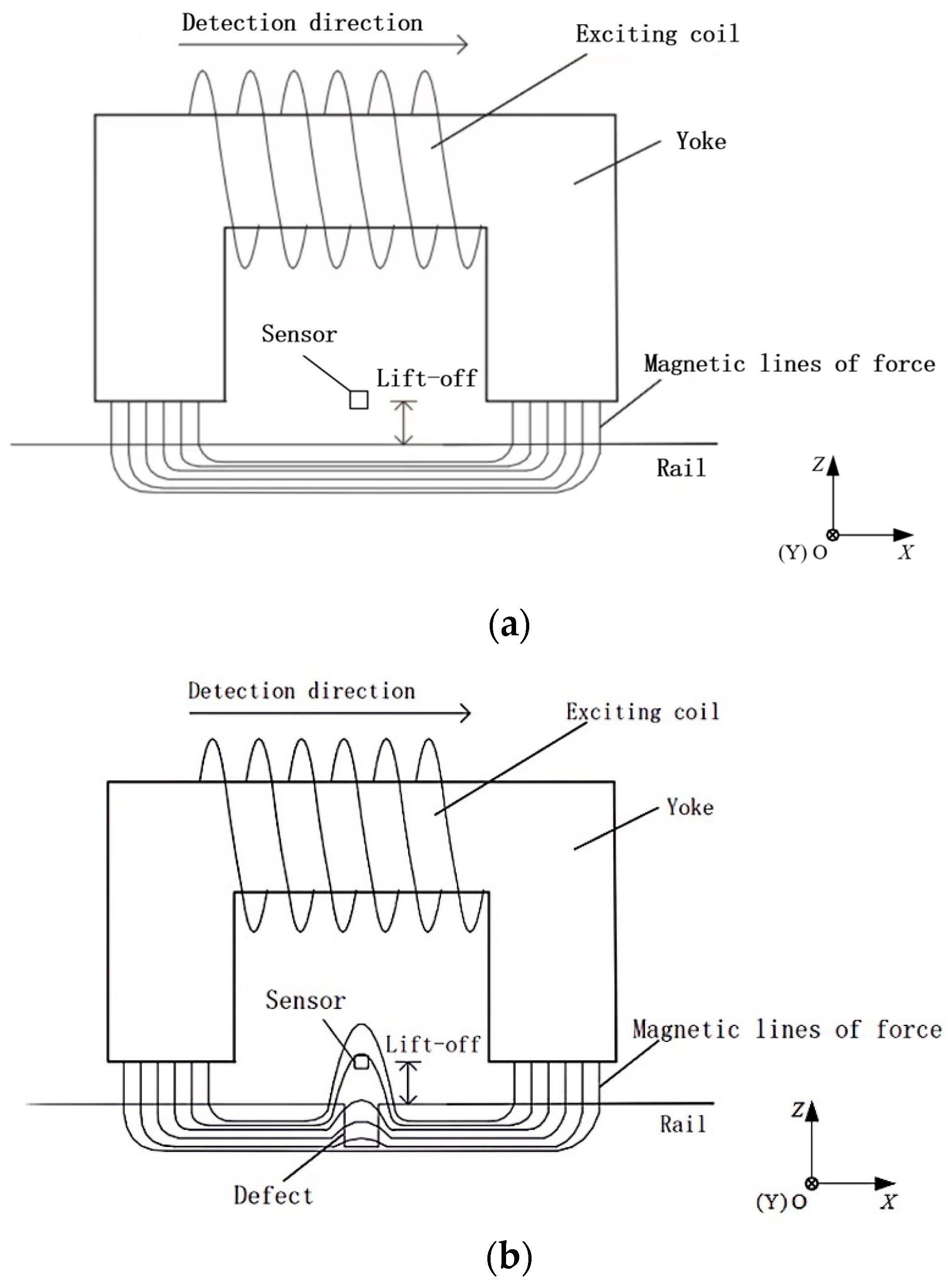
The MFL detection principle and the coordinates used in this article are shown in Figure 1. The detection probe moves above the rail, which is partially magnetized by the external magnetic field. When the rail surface is flat and undamaged, the magnetic lines will be constrained inside the rail, as Figure 1a shows. If a defect is in the rail surface or subsurface, as Figure 1b shows, due to the magnetic permeability of ferromagnetic materials being greater than that of air, some magnetic lines refract at the interface between the rail and air, creating a leakage magnetic field in the external space near the defect [3]. The defect can be detected by picking up the leakage magnetic field signal near the rail surface using a sensor. This article takes the filtering of the MFL detection signal in the x-direction as an example as an introduction.

Early defects are often small, and the excitation magnetic field should not be too strong to prevent the rail from being permanently magnetized. So, the MFL signal is often weak and interfered with by various noise sources. The vertical distance from the sensor or yoke to the rail is called lift-off. When the probe moves, the lift-off of the sensor or yoke will change due to vehicle vibration, which will interfere with detection. Vibration noise is the strongest interference during detections. In addition, there are other interferences, such as system noise, noise caused by velocity effect, random interference, etc. [4]. High background noise and low signal-to-noise ratio (SNR) bring difficulties for subsequent defect assessment. Therefore, signal filtering is required.

With the proposal and improvement of various filtering algorithms, many methods have been applied to filter MFL signals.

Donoho D.L. [5] proposed the method of wavelet transform (WT). For MFL signal processing, the algorithm improvements in WT are often made by modifying soft and hard thresholds, wavelet coefficients, and other methods, or combined with median filtering, adaptive filtering, and other methods to achieve better filtering results. For example, Afzal M. et al. [6] combined WT with adaptive filtering to filter the MFL signal of seamless steel pipes. The method has advantages such as adaptability and a fast convergence speed. Zhang [7] proposed a multi-level filtering method that combined median and wavelet filtering to improve the MFL detection accuracy. The experimental results show that the method has a good filtering effect.

Song et al. [8] proposed a filtering method based on the wavelet packet and threshold algorithm for signals of crack defects in oil and gas pipelines. The high-frequency wavelet coefficients were organized into a tree structure, and the wavelet coefficient tree was trimmed by setting a threshold to suppress high-frequency noise while ensuring the integrity of the high-frequency signal. Ji et al. [9] compared the filtering performance of improved wavelet packets processed using a hard, soft, and fuzzy threshold, and finally applied the fuzzy threshold to achieve MFL signal filtering.

Huang N. E. et al. [10] proposed empirical mode decomposition (EMD). According to the characteristics of the signal itself, the method adaptively decomposes the signal into a series of intrinsic mode components and sums these components to obtain the filtered signal. EMD has good adaptability and does not rely on pre-defined basis functions, making it suitable for the decomposition and analysis of nonlinear and non-stationary signals, such as MFL signals. To improve EMD, many methods have been proposed.

Smith J. S. [11] proposed local mean decomposition (LMD), which suppressed endpoint effects and modal aliasing in EMD while improving the decomposition accuracy. Huang N. E. et al. [12] proposed ensemble empirical mode decomposition (EEMD). By adding white noise multiple times to the signal to weaken the modal aliasing caused by impact interference, more precise upper and lower envelopes were obtained, improving the decomposition accuracy. Yeh J. R. et al. [13] proposed complementary ensemble empirical mode decomposition (CEEMD) based on EEMD. By adding a pair of white noise sources, opposite to each other, to the signal, the improved method solves the modal aliasing problem while ensuring that white noise is eliminated from the reconstructed signal. Zosso D. et al. [14] transformed the signal decomposition problem into a variational solution problem and proposed variational mode decomposition (VMD), which can suppress modal aliasing and has good noise robustness.

In addition, Yang et al. [15] proposed a filtering method for the MFL signal based on EMD and wavelet filtering. The decomposed components of the MFL signal were wavelet-filtered and reconstructed, achieving good SNR. Chen et al. [16] proposed an MFL signal image-filtering method based on the combination of mean filtering and bidimensional empirical mode decomposition (BEMD). The bidimensional intrinsic mode functions decomposed by BEMD are then mean-filtered and reconstructed to obtain high-SNR MFL images.

Combining the tightly supported framework of WT with the adaptive concept of EMD, Gilles J. [17] proposed empirical wavelet transform (EWT) based on narrowband signal analysis theory and WT. Non-iterative methods are used for the signal decomposition. EWT provides a time–frequency analysis approach for constructing adaptive wavelets for signal processing, continuously used and improved, and gradually applied in signal processing. Basing on spectral kurtosis and EWT, Hu et al. [18] proposed an adaptive partial discharge fluorescence signal-filtering algorithm. By using a fast spectral kurtosis graph to merge the tightly supported regions of the noisy signal, the Fourier spectrum of the noisy signal is re-divided, reducing the division of invalid noise components and thus reducing the computational cost of the algorithm. Tang et al. [19] proposed an improved adaptive parameterless EWT filtering method that combined mutual information (MI) and spline interpolation fitting to optimize spectrum division. The method effectively suppressed noise in the high-frequency partial-discharge signals of transformers.

At present, MFL signal processing has achieved fruitful results, but its application mainly focuses on steel wire ropes, oil and gas pipelines, steel pipes, etc. There is less discussion in the field around the non-destructive detection of rails [20]. EWT combines the advantages of EMD and WT, and is suitable for processing nonlinear and non-stationary signals. Due to rail-surface-defect MFL signals being nonlinear and non-stationary, EWT is suitable for the analysis, and it may also result in a better processing efficiency by improving EWT. However, the rail is long, and the detection speed is always faster than that of a rope or pipeline, so the interferences are different. In this work, the suppression of the vibration noise and random interference while maintaining the same inspection speed is studied, and a method for rail-head surface-defect MFL signal filtering based on improved EWT via MI and kurtosis is proposed to suppress the defect signal background noise and improve the SNR.

2. Improved EWT

2.1. EWT

Perform fast Fourier transform (FFT) on the original signal f(t), then normalize the frequency range of the Fourier spectrum within 2π. According to the Shannon criterion, only discuss the characteristics within the interval [0, π] during the signal analysis. Using the scale space method to adaptively divide the Fourier spectrum into continuous N intervals within [0, π], next, obtain $N+1$ interval boundaries, using ${\omega }_n$ to represent boundaries, where ${\omega }_0=0$, ${\omega }_n=\pi$, and using ${\Lambda }_n$ to represent divided intervals, that is:

$${\Lambda }_n=[{\omega }_{n-1},{\omega }_n],n=1,2,\dots ,N$$

(1)

Add wavelet windows to ${\Lambda }_n$. Establish the bandpass filter bank based on Littlewood–Paley and Meyer wavelet [17]. When $n>0$, define the empirical wavelet function ${\psi }_n(\omega )$ and empirical scale function ${\phi }_n(\omega )$ as Formulas (2) and (3), where

$${\psi }_n(\omega )=\left\{\begin{array}{ll}\begin{array}{l}1,\\ \end{array}\hfill & \begin{array}{l}{\omega }_n+{\tau }_n\le \left|\omega \right|\le {\omega }_{n+1}-{\tau }_{n+1}\\ \end{array}\hfill \\ \begin{array}{l}\cos \left[\frac{\pi }{2}\beta \left(\frac{1}{2{\tau }_{n+1}}\left(\left|\omega \right|-{\omega }_{n+1}+{\tau }_{n+1}\right)\right)\right],\\ \end{array}\hfill & \begin{array}{l}{\omega }_{n+1}-{\tau }_{n+1}\le \left|\omega \right|\le {\omega }_{n+1}+{\tau }_{n+1}\\ \end{array}\hfill \\ \begin{array}{l}\sin \left[\frac{\pi }{2}\beta \left(\frac{1}{2{\tau }_n}\left(\left|\omega \right|-{\omega }_n+{\tau }_n\right)\right)\right],\\ \end{array}\hfill & \begin{array}{l}{\omega }_n-{\tau }_n\le \left|\omega \right|\le {\omega }_n+{\tau }_n\\ \end{array}\hfill \\ 0,\hfill & \mathit{others}\hfill \end{array}\right.$$

(2)

$${\phi }_n(\omega )=\left\{\begin{array}{ll}\begin{array}{l}1,\\ \end{array}\hfill & \begin{array}{l}\left|\omega \right|\le {\omega }_n-{\tau }_n\\ \end{array}\hfill \\ \begin{array}{l}\cos \left[\frac{\pi }{2}\beta \left(\frac{1}{2{\tau }_n}\left(\left|\omega \right|-{\omega }_n+{\tau }_n\right)\right)\right],\\ \end{array}\hfill & \begin{array}{l}{\omega }_n-{\tau }_n\le \left|\omega \right|\le {\omega }_n+{\tau }_n\\ \end{array}\hfill \\ 0,\hfill & \mathit{others}\hfill \end{array}\right.$$

(3)

where $\beta (x)$ is a polynomial that satisfies the transformation of Formulas (2) and (3) above. Its expression is β(x) = x⁴ (35 − 84x + 70x² − 20x³).

Empirical wavelet coefficients include approximation and detail coefficients. The approximation coefficients $W_f^e(0,t)$ are inner products of $f(t)$ and ${\phi }_1(\omega )$; the detail coefficients $W_f^e(n,t)$ are inner product of $f(t)$ and ${\psi }_n(\omega )$.

$$W_f^e(0,t)=〈f,{\phi }_1〉={\displaystyle \int f}(\tau )\overline{{\phi }_1(\tau -t)}d\tau =F^{-1}\left[f(\omega )\overline{{\phi }_1(\omega )}\right]$$

(4)

$$W_f^e(n,t)=〈f,{\psi }_n〉={\displaystyle \int f}(\tau )\overline{{\psi }_n(\tau -t)}d\tau =F^{-1}\left[f(\omega )\overline{{\psi }_n(\omega )}\right]$$

(5)

After decomposing $f(t)$, the AM-FM single components from low to high frequency can be obtained as follows:

$$f_0(t)=W_f^e(0,t)\ast {\phi }_1(t)$$

(6)

$$f_k(t)=W_f^e(k,t)\ast {\psi }_k(t), k=1,2,\dots ,N$$

(7)

Finally, the expression for the reconstructed signal is:

$$f(t)={\displaystyle \sum _{n=0}^N}{f}_n(t)=W_f^e{(0,t)}^{\ast }{\phi }_1(t)+{\displaystyle \sum _{n=1}^N{W}_f^e}{(n,t)}^{\ast }{\psi }_n(t)$$

(8)

2.2. A Boundary-Optimization Method Based on MI

Spectrum division is the basis for signal reconstruction and determines the quantity and quality of the decomposed signals. Due to the adaptive decomposition process of EWT, the signal boundary may be redundant if the signal is complex, such as the MFL detection signal, with vibration noise and other interferences. The redundant boundary leads to the obtention of unnecessary components and disrupts the integrity of the spectrum. In order to reduce the boundary redundancy in EWT, a boundary optimization method based on MI is proposed.

MI considers the mutual independence between variables from the perspective of probability distribution. Assuming that two random variables are $X$ and $Y$, MI can quantitatively represent the degree of interdependence between the two, where

$$MI(X,Y)=H(Y)-H(Y|X)$$

(9)

$MI(X,Y)$ is the MI of $X$ and $Y$, $H(Y)$ is the entropy of $Y$, and $H(Y|X)$ is the entropy of $Y$ under the condition of $X$. The stronger the correlation between $X$ and $Y$, the smaller the $H(Y|X)$, and the greater the $MI(X,Y)$.

After dividing the spectrum using the scale space method to obtain some initial components, the correlation between each component and the original signal based on MI is calculated. The initial components are screened via correlation, and the spectrum is redivided to eliminate redundant components.

The boundary-optimization process is shown in Figure 2. Let i represent any one of the initial components, and component $i-1$ and $i+1$ are the adjacent components of component i. Suppose MI_i is the MI between component i and the original signal $f(t)$, MI_m is the mean of all the MI_i. Calculate each MI_i and compare it with MI_m. If MI_i > MI_m and MI_i+1 > MI_m, or MI_i ≤ MI_m and MI_i+1 ≤ MI_m, then merge component i and $i+1$. If MI_i > MI_m and MI_i−1 > MI_m, or MI_i ≤ MI_m and MI_i−1 ≤ MI_m, then merge component i and $i-1$. Otherwise, the components remain independent. After merging, some new boundaries can be obtained to re-divide the spectrum.

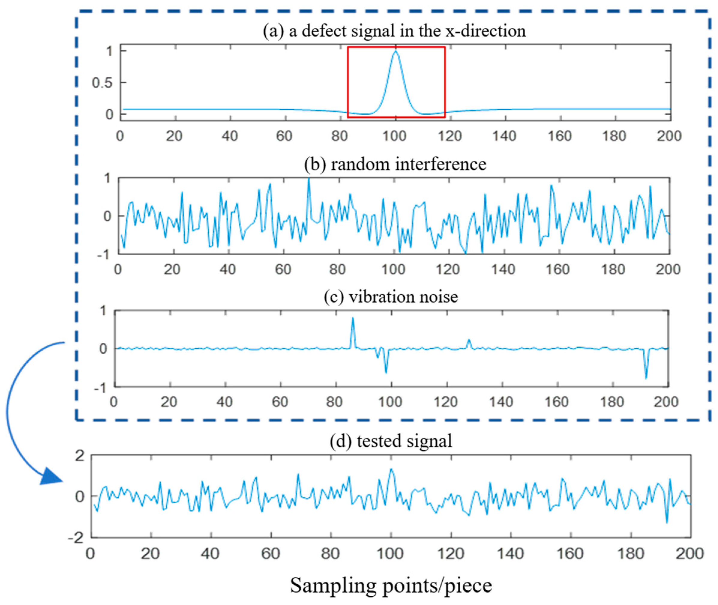
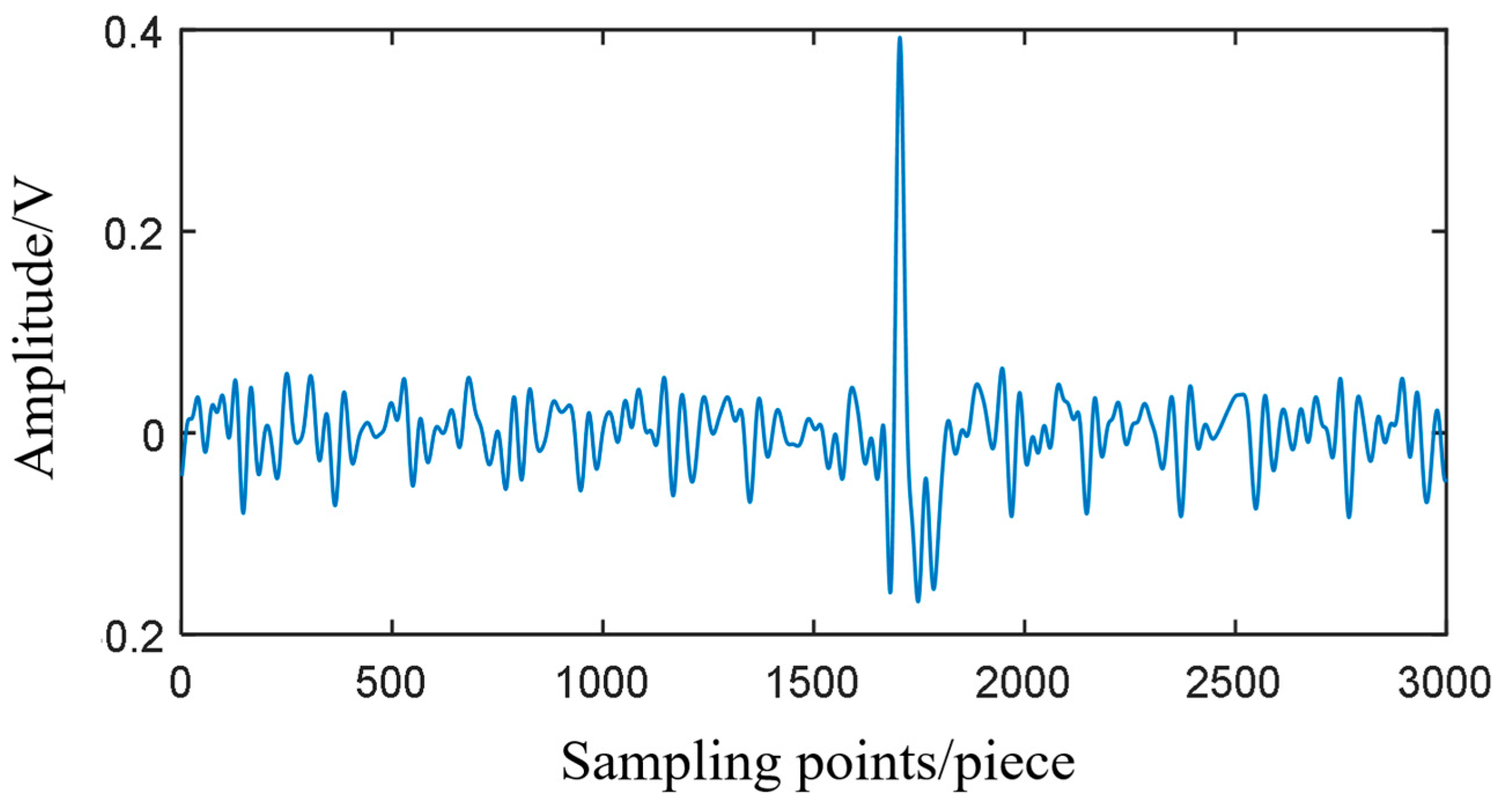
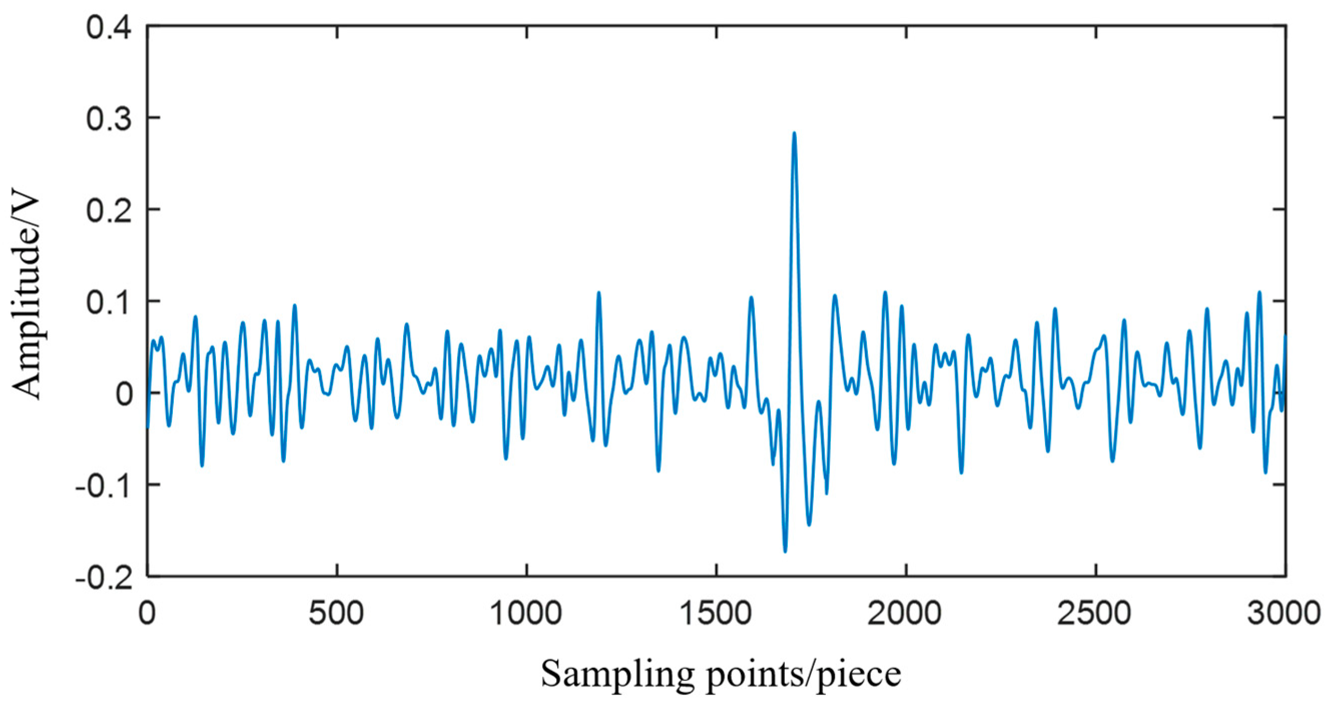
Here is an example to introduce this method. The signal consists of three components: a defect MFL signal in the x-direction, as show in a red rectangle in Figure 3, a random interference, and vibration noise.

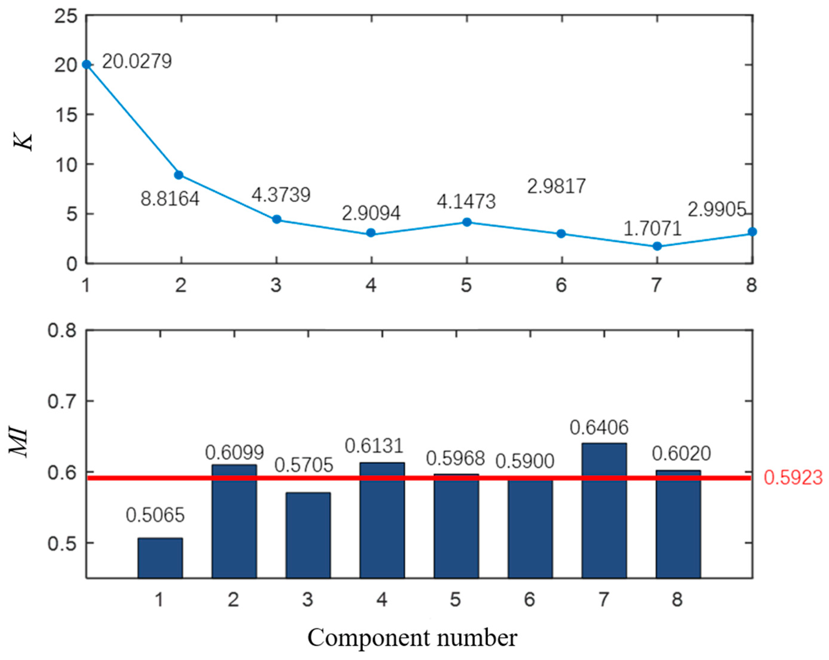
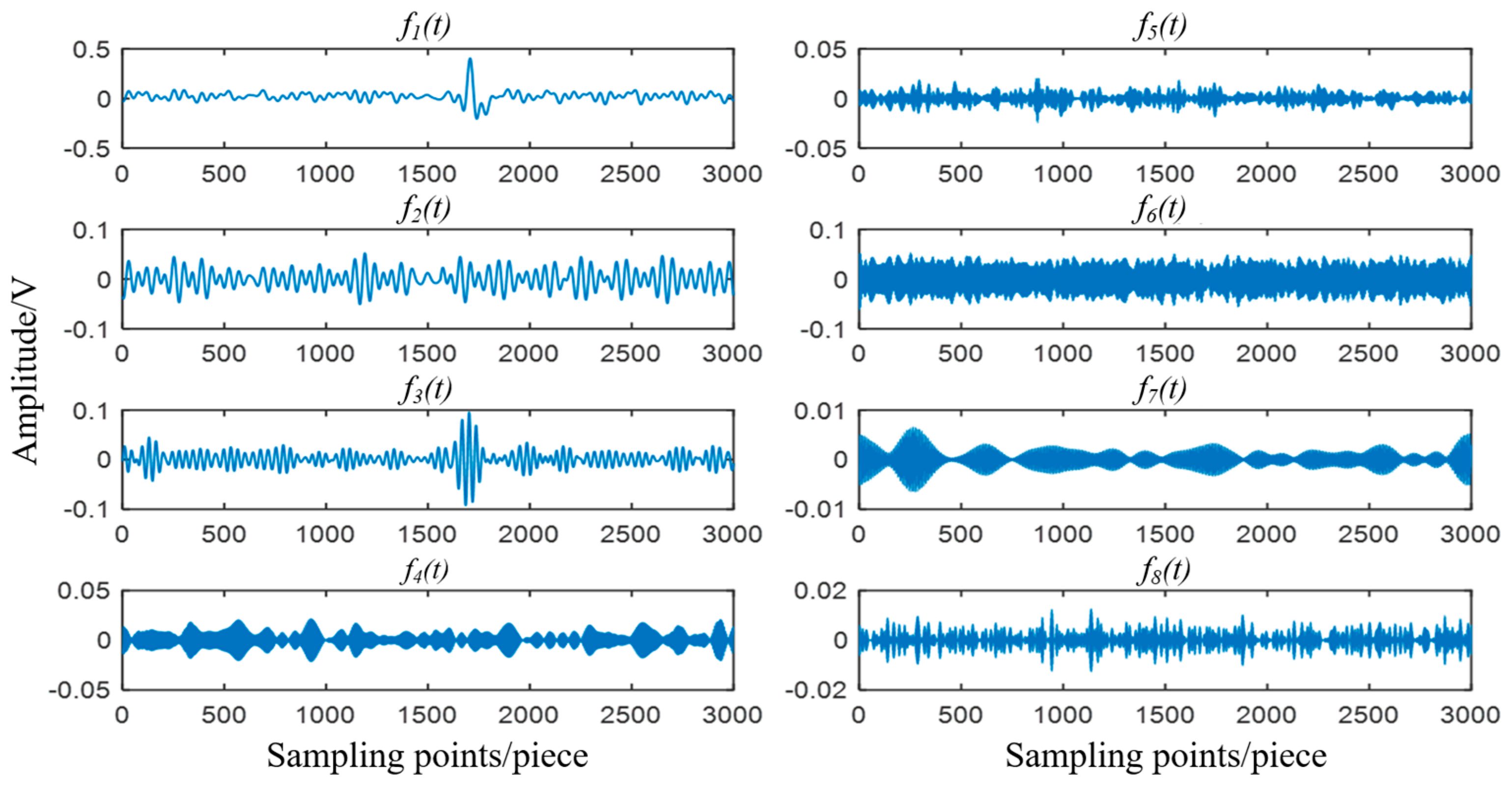
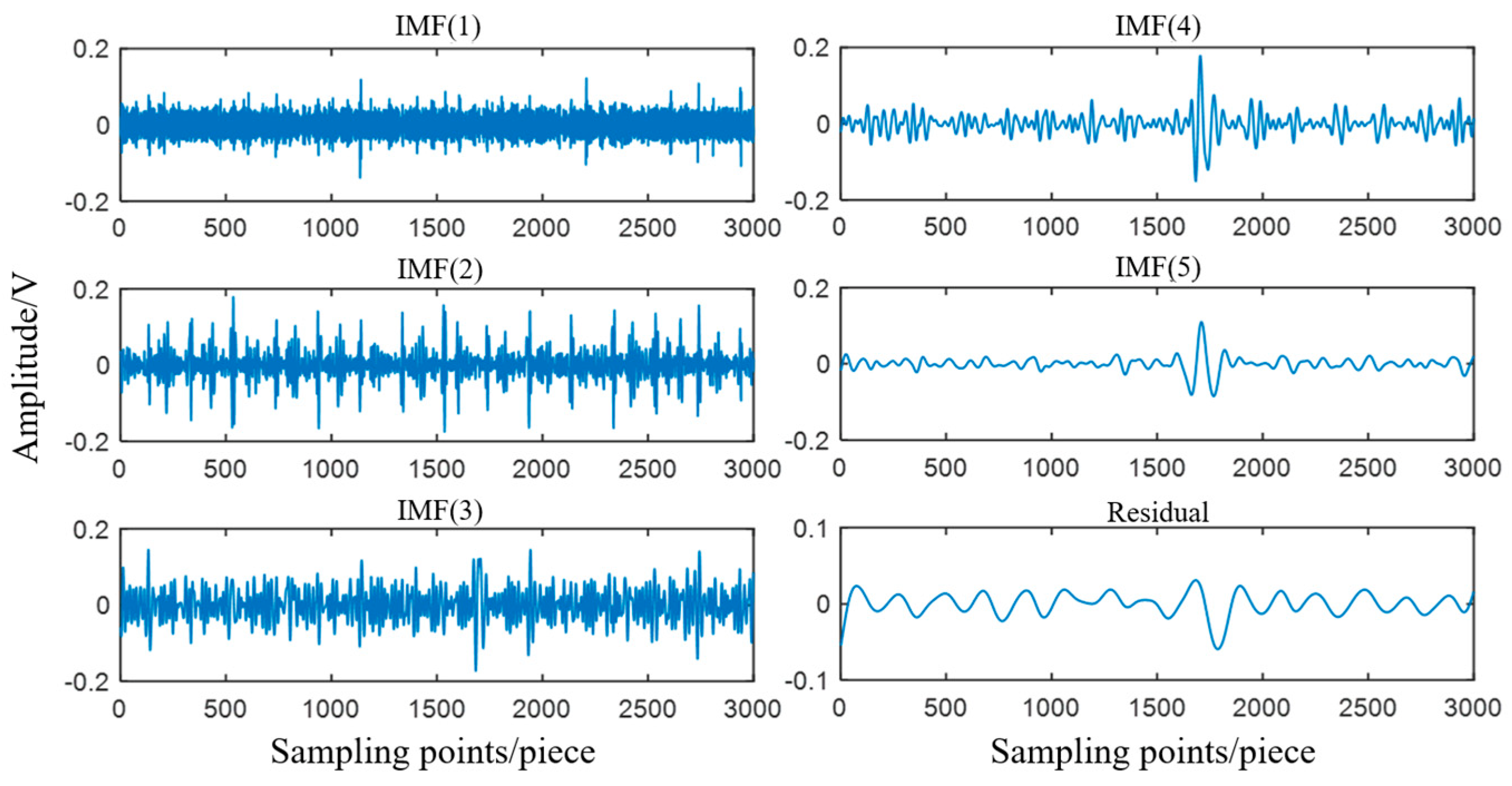
The signal was adaptively divided into 23 initial components using the scale space method. Some components were redundant. MI_i were calculated and are shown in Figure 4. MI_m is marked with a solid red line, and the new boundaries obtained via the boundary-optimization method are marked with dashed red lines. After re-dividing the spectrum, we constructed a filter bank according to Equations (2) and (3) to obtain four modal components, as shown in Figure 5. Record the new components as $f_n\left(t\right)$.

According to the principle of MI and the composition characteristics of the signal, the larger the MI_i, the more noise ingredients unrelated to defect information are contained in the component i. From the bar graph of MI_i, it can be seen that the first component is located in the low-frequency part and has the smallest MI, indicating that it has the smallest correlation with the tested signal. Meanwhile, combined with Figure 3, a significant peak appears at the defect location, as shown in a red rectangle in Figure 5, indicating that this component contains a defect signal.

The defect component, vibration noise component, and random interference component in the signal are successfully separated, and the number of components is reduced from the initial 23 to 4. Obviously, this method has no redundant components and decomposes signals accurately.

2.3. Component Selecting Based on MI and Kurtosis

After re-dividing the spectrum through the boundary-optimization method and decomposing $f(t)$, it is necessary to select suitable components containing the defect signal for signal reconstruction. MI reflects the relationship between each component and $f(t)$. From Figure 4, it can be observed that MI between $f_1(t)$ and $f_n(t)$, and MI between $f_3(t)$ and $f_n(t)$ should be both less than MI_m, which is more likely to include defect signals. However, as shown in Figure 5, $f_3(t)$ is distributed in the high-frequency region, and from the frequency-domain perspective, the possibility of $f_3(t)$ containing a defect signal is extremely low. Therefore, if the components selected are only based on MI, components without a defect may be selected, resulting in the reconstructed signal still containing high interference. Therefore, in addition to MI, kurtosis is also used to select the suitable components.

Kurtosis is a dimensionless parameter that characterizes a signal waveform’s peak degree. For an arbitrary input signal $x$, define the kurtosis as:

$$K=\frac{E{(x-{\mu }_0)}^4}{{\sigma }^4}$$

(10)

${\mu }_0$ is the mean of $x$. $\sigma$ is the standard deviation of $x$. $E(·)$ represents compute the mathematical expectation.

K is very sensitive to the mutagenic component in a signal. If a signal approximately follows normal distribution, then K is about 3, such as Gaussian white noise. If a signal has an impact or protrusion, then K is greater than 3. Therefore, when using kurtosis to analyze the defect MFL signal, the K of the signal has the following characteristics: if no defect is detected, the signal only contains noise, and its amplitude is close to normal distribution, then K is about 3. If some defects are detected, the signal has obvious protrusions, and does not follow normal distribution, then K is greater than 3. The steeper the peak value of the signal, the greater the K. A large number of detection data have been studied, and this pattern has been proven to be correct.

The process of components selecting is as shown in Figure 6:

(1)

Calculate MI between components $f_n\left(t\right)$ and $f\left(t\right)$, and calculate K of $f_n\left(t\right)$.

(2)

Compare each MI with the mean MI_m and K of each $f_n\left(t\right)$ with 3. The components whose MI is not greater than MI_m and K is greater than 3 are retained. Other components are deleted.

(3)

Reconstruct the undeleted components according to Equation (8) to obtain the reconstructed signal.

The MI and K of each component in Figure 5 are shown in

Table 1. MI and K of each component.

	MI	K
f1(t)	0.8001	5.4834
f2(t)	0.8235	2.8071
f3(t)	0.8162	2.7437
f4(t)	0.8432	1.9591
mean	0.8208	--

. Firstly, by comparing each MI with MI_m, $f_1(t)$ and $f_3(t)$ are selected. And then, observing K of the two, only the K of $f_1(t)$ is greater than 3. Therefore, only $f_1(t)$ is retained, and other components are deleted. The reconstructed signal is $f_1(t)$.

2.4. Process of Defect MFL Signal Filtering

A boundary-optimization method is proposed to reduce boundary redundancy in spectrum division, and a component-selection method is proposed to screen out the suitable components for signal reconstruction. The following is the overall filtering process:

(1)

Operate the original MFL signal with FFT to get the Fourier spectrum, and divide the spectrum into several components via the scale-space method.

(2)

Re-divide the spectrum into new components via the boundary optimization method.

(3)

Select suitable components among the new components based on the MI and K.

(4)

Reconstruct the signal.

3. Experimental Results and Analysis

3.1. Experimental Devices and Materials

The data used in the article were collected using a detection train. The detection device consists of a detection probe, a conditioning circuit, a signal data acquisition card, and a computer. The detection probe is mainly composed of a magnetizer, a sliding shoe, and a Hall sensor array. The Hall sensor array is situated between the sliding shoe and magnetizer, as shown in Figure 7. The device is installed on the train and scans along the railway. During detection, the lift off will vary within 1–3 mm.

Figure 8 shows a defect, with a length of approximately 15 mm in the x-direction and a width of approximately 13 mm in the y-direction. The detection speed was 45 km/h. The original signal collected via the probe is shown in Figure 9, and the defect MFL signal is marked with a rectangle on the graph.

3.2. Results and Discussion

The signal was operated with FFT, and its spectrum was adaptively divided into 50 initial components. We re-divided the spectrum via the boundary optimization method, as shown in Figure 10. We constructed a filter bank to obtain a new set of components, as shown in Figure 11.

The MI and K of each component after re-dividing the spectrum are shown in Figure 12. First, according to MI_m, the components $f_1(t)$, $f_3(t)$, and $f_6(t)$ were selected. And then, according to K, $f_1(t)$ and $f_3(t)$ were finally selected. The two components were used to reconstruct the signal according to Equations (2) and (3). Figure 13 shows the reconstructed signal.

From Figure 13, obviously, after filtering, the defect signal component was retained and noise interference was suppressed compared to Figure 9. To verify the advantage of the improved EWT in minor-defect MFL signal filtering, CEEMD and WT were used to filter the defect signal, and the filtering effects of the three methods were compared.

(1)

CEEMD

The IMF components and residual component obtained by decomposing the defect signal using CEEMD are shown in Figure 14. We selected the suitable components according to the method in Figure 6, and the reconstructed signal is shown in Figure 15.

(2)

WT

There have been studies on the filtering of the MFL signal using WT, including the aspects of wavelet basis and decomposition layers. According to Ref. [21], we selected sym6 as the wavelet basis, set the number of layers for wavelet decomposition to 10, and adopted the soft threshold processing method. Figure 16 shows the WT filtering result.

The common evaluation indicators of filtering quality for the defect signal include SNR and root-mean-square error (RMSE), etc. [21]. The filtering effects of improved EWT, CEEMD, and WT were compared via SNR and RMSE. The results are shown in

Table 2. Processing effects of different methods.

	SNR (dB)	RMSE (V)
The original signal	−20.79	0.090
Improved EWT	−5.25	0.036
CEEMD	−8.71	0.053
WT	−12.81	0.063

. Because of the strong background noise and weak defect signal, the power of the useful signal is lower than that of the noise, resulting in a negative SNR. From Table 2, it can be seen that after being processed via the improved EWT, the SNR is increased by 15.54 dB compared to that of the original signal, and is 3.46 dB and 7.46 dB higher than that of CEEMD and WT, respectively. The RMSE has decreased by 60% compared to that of the original signal. It can be concluded that the improved EWT proposed in this article can preserve defect signal components while suppressing background noise, and has a better performance compared to CEEMD and WT.

4. Conclusions

This article proposes an improved EWT method to filter rail-head surface-defect MFL signals. Based on MI, a boundary-optimization method is designed to reduce the boundary redundancy caused by adaptive spectrum division in EWT. A component-selecting method is proposed based on MI and kurtosis, which enables the selection of the components with defects from the decomposed components for reconstructing the signal. Experimental verification was conducted on the detection data collected using a detection train. The results show that the improved EWT proposed in this article has an obvious effect on filtering the rail-head surface-defect MFL signal, with a higher SNR and smaller RMSE compared with CEEMD and WT. In the future, reconstruction and evaluation methods for defects based on filtered signals will be studied.