LSTM with Short-Term Bias Compensation to Determine Trading Strategy under Black Swan Events of Taiwan ETF50 Stock

Abstract

This paper uses Long Short-Term Memory (LSTM) networks to predict the stock prices of the Yuanta Taiwan Top 50 ETF (ETF50). To improve the accuracy of the model’s predictions, a calibration procedure called “Short-Term Bias Compensation” (STBC) is proposed to adjust the predicted stock prices. In STBC, the daily prediction error is calculated to estimate the short-term bias (STB) in prediction. Then, the predicted price of its next day will be corrected if this STB has exceeded a certain threshold. In this paper, we apply Genetic Algorithms (GAs) to optimize the parameters used in STBC for providing more confidence in its estimation. Based on these predicted stock prices, we propose a Genetic Fuzzy System (GFS) to determine the trading strategy, with trading points for buying and selling stocks. In GFS, various technical indicators are used to establish the fuzzy rules of the trading strategy, and GAs are used to evolve the best parameters for these fuzzy rules. Our experiments cover over 17 years of data (from 2003 to 2020) for ETF50 to consider black swan events such as the 2020 COVID-19 pandemic, the 2018 US–China trade war, and the 2011 US debt crisis. The first 90% of the data is used as training data, and the last 10% is used as testing data. We use 12 technical indicators of these data as the input of LSTM. The predicted values of LSTM are corrected using STBC and compared to the uncorrected prices. We use Mean Square Error (MSE) to evaluate the prediction accuracy. The results show that STBC can nearly reduce 90% of the prediction error (where MSE drops from 11.5758 to 1.2687). By using GFS with STBC to determine trading points, we achieve a return rate of 32.0%.

1. Introduction

This paper uses the “Yuanta/P-shares Taiwan Top 50 ETF (Exchange Traded Fund)” (ETF50) [1] as the research target. It tracks Taiwan’s top 50 stock index and holds the same constituent stocks as the top 50 index in Taiwan. This paper primarily focuses on the technical analysis of stocks, using the performance of technical indicators to understand the current state of the stock market. To achieve higher returns, investors aim to buy stocks at low prices and sell them at high prices. In past years, different studies were proposed to determine the trading points for buying and selling, serving as a stock trading strategy [2]. However, during certain black swan [3] events or periods of extreme market volatility, traditional rules that simply apply stock technical indicators [4] may not yield satisfactory trading results. For example, the 2020 COVID-19 pandemic [5], the 2018 US–China trade war, and the 2011 US debt crisis have greatly impacted financial markets, making it challenging for investors to achieve good returns.

The ETF50 considers 50 listed companies in Taiwan, among which TSMC (Taiwan Semiconductor Manufacturing Company) holds the most important position and determines much of the stock market trend. TSMC plays a pivotal role not only in Taiwan’s economy but also in the global semiconductor industry. As the largest contract chip manufacturer in the world, TSMC competes with other major players such as Intel, Nvidia, Samsung, and Philips. In terms of technological advancements and production capacity, TSMC has consistently maintained a leadership position, particularly in advanced node technology, such as 5 nm and 3 nm processes, which are critical for manufacturing next-generation chips used in smartphones, AI, and autonomous vehicles.

The COVID-19 pandemic significantly disrupted the global semiconductor supply chain. Lockdowns, workforce shortages, and surging demand for consumer electronics, such as laptops and smartphones, caused a global chip shortage that impacted industries from the automotive industry to telecommunications. TSMC, with its advanced manufacturing capabilities, was pivotal in addressing the shortage, but the gap between supply and demand persists. This situation highlighted the dependence of global industries on a few key manufacturers, like TSMC and Samsung, which continue to face pressure to ramp up production amidst geopolitical tensions and increasing global demand.

Traditional stock prediction models, including time-series analysis and statistical methods, largely rely on historical data and the assumption that future market movements will remain within predictable bounds. However, black swan events defy these assumptions, making such models ineffective in extreme scenarios. The inability of these models to account for rare and unexpected events often results in flawed predictions, especially during periods of heightened market volatility. Consequently, there is a growing need to explore deep learning techniques, which can adapt to a wider range of data and learn more complex, nonlinear patterns, to better handle the unpredictability of black swan events.

This paper uses a calibration procedure called “Short-Term Bias Compensation” (STBC) to adjust the model’s stock price predictions, aiming to reduce the impact of sudden external factors on the model’s prediction accuracy. We use fuzzy rules [6] evolved by genetic algorithms (GAs) to determine the stock trading strategy. The basic processing steps of this paper are as follows.

• Predict Stock Prices: This paper employs a deep learning Long Short-Term Memory (LSTM) model [7] to predict stock prices. LSTM is particularly useful for handling time-series data, making it a powerful tool for financial market prediction [8]. By training on historical stock data through multiple neurons and multiple layers of the network, it learns the stock price trends to predict future stock prices.
• Calibrate Prediction: Due to the LSTM prediction error, this paper uses STBC to adjust the predicted stock prices by avoiding inaccuracies caused by stock price volatility. It thereby achieves the goal of reducing model prediction errors.
• Determine Trading Points: This paper uses GAs to evolve the optimal parameters of the membership functions of fuzzy rules to form a fuzzy system, which determines the buying and selling points.
• Optimize Trading Strategy: The predicted lowest and highest prices are used as the buying and selling prices for executing trades.

In financial markets, stock price prediction is not only critical for investors’ trading decisions but also helps assess the financial health of companies, thereby predicting bankruptcy risk. The Z-Score model [9], widely used for bankruptcy prediction, is based on financial ratios that assess a company’s risk of insolvency. These ratios include operating capital, reinvested income, earnings before interest and taxes, market value of equity, and sales revenue, all of which reflect a company’s stability and debt-paying ability. Therefore, stock price fluctuations are not only tied to market sentiment and supply–demand dynamics but also have a close relationship with the underlying financial risks of a company.

This study aims to predict stock prices of the Taiwan Stock Exchange ETF50 using LSTM networks with STBC calibration. By training on historical stock data, we can learn market trends and further estimate a company’s financial status and bankruptcy risk. Such a stock prediction model provides investors with a deeper risk management perspective, particularly in volatile markets, enhancing decision-making accuracy.

This paper is divided into five sections. Section 1 addresses the research motivation of the paper. Section 2 introduces the relevant literature on LSTM, fuzzy systems, GAs, and stock trading strategies. Section 3 explains the experimental process and framework to determine the trading points and the trading strategy. Section 4 presents the experimental results and analysis, identifying the optimal trading strategy. Finally, Section 5 summarizes the research findings and discusses any shortcomings and possible directions for future improvements and extensions.

2. Related Works

2.1. Long Short-Term Memory (LSTM)

Due to the gradient explosion and vanishing problems in Recurrent Neural Networks (RNNs) [10], which result in poor model training effectiveness, Sepp Hochreiter and Jürgen Schmidhuber proposed LSTM in 1997 [7]. LSTMs have three types of gates: Forget Gate, Input Gate, and Output Gate.

The Forget Gate f_t determines whether to retain or forget the memory unit c_t−1 from the previous time step. The current input value x_t and the previous hidden state h_t−1 are multiplied by a weight matrix and the result is passed through a sigmoid function. The output value f_t ranges between 0 and 1, with higher values indicating a higher probability of retention and lower values indicating a higher probability of forgetting.

$$f_t=sigmoid\left({W_{f}x}_t+U_f{h}_{t-1}+b_f\right)$$

(1)

The Input Gate controls the current input. The previous hidden state h_t−1 and the current input value x_t are multiplied by a weight matrix and passed through a hyperbolic tangent tanh function to get $\tilde{c}$_t. Simultaneously, $\tilde{c}$_t is input into the sigmoid function to get i_t, which decides which information from $\tilde{c}$_t should be retained.

$${\tilde{c}}_t=tanh\left(W_c{x}_t+{U_{c}h}_{t-1}+b_c\right)$$

(2)

$$i_t=sigmoid\left(W_i{x}_i+{U_{i}h}_{t-1}+b_i\right)$$

(3)

$$h_t=o_t\times tanh\left(c_t\right)$$

(4)

The Update Long-Term Cell State c_t is described as follows. The previously calculated i_t and $\tilde{c}$_t are multiplied to determine if the cell should be updated. The output value f_t from the Forget Gate is multiplied by the previous cell state c_t−1 and then added to the current i_t multiplied by the new cell state $\tilde{c}$_t.

$$c_t=i_t\times {\tilde{c}}_t+f_t\times c_{t-1}$$

(5)

The Output Gate determines the hidden state value h_t for the next layer. The current input value x_t and the previous hidden state h_t−1 are calculated through the sigmoid activation function to determine whether the current memory unit c_t is output as o_t. Finally, the output value o_t from the Output Gate is obtained.

$$o_t=sigmoid\left({W_{o}x}_t+{U_{o}h}_{t-1}+b_o\right)$$

(6)

2.2. Fuzzy Systems

Fuzzy theory uses mathematical methods to address issues related to ambiguous semantics. In everyday life, people’s descriptions of things can vary. For instance, one person might consider the weather cold if it is below 18 °C, while another might feel it is cold when it is only below 20 °C. Similarly, in restaurant reviews, some might rate the food as excellent with a score of nine, while others might rate it as good with a score of seven. These differences in perception create ambiguity and fuzziness in descriptions, which fuzzy theory can handle effectively.

Fuzzy control utilizes fuzzy sets, fuzzy logic, and fuzzy inference to deal with ambiguity and uncertainty. Unlike traditional control theory, which relies on precise mathematical models and inputs, fuzzy control can function without such constraints. It uses expert knowledge, rules, and experience for control settings. The input values are fuzzified, transforming them into fuzzy sets. Through the fuzzy inference engine, based on a knowledge base and fuzzy rules, the inputs are processed and, finally, the results are defuzzified to obtain concrete outcomes.

Fuzzification maps input values to fuzzy sets using membership functions to express the degree to which each value belongs to a fuzzy set. This process converts precise input values into a form suitable for fuzzy logic processing. Fuzzy sets are mathematical functions representing ambiguity and uncertainty. Elements are associated with the functions, and their membership values are calculated. The membership value indicates the degree of association between an element and the set; the closer the element is to the set, the higher its membership value. Common membership functions [11] include Gaussian, triangular, trapezoidal, S-function, Z-function, and Pi-function. The choice of function depends on the specific needs.

After fuzzification, the fuzzy inference engine performs reasoning based on rules from the rule base and knowledge base. The engine [12] uses the membership functions and conditions of the input values to compute their membership values. The rule base consists of a series of IF–THEN rules, where each rule has an “IF” condition and a corresponding “THEN” action. These rules are defined based on expert knowledge, experience, or extensive data collection.

The fuzzy inference engine uses the knowledge base and rules to infer fuzzy results. Defuzzification then converts these fuzzy results into specific outcomes, yielding the most reasonable results and achieving the purpose of establishing a fuzzy system. Common defuzzification methods include the Center of Maximum (CoM), Center of Area (CoA), and Mean of Maximum (MoM). CoM uses the highest membership value as the central point for defuzzification. CoA treats the membership function of the fuzzy set as an area and calculates the center of this area for defuzzification. MoM averages the elements with the highest membership values for defuzzification. These methods ensure that the defuzzified results are consistent with the inferred fuzzy outcomes.

2.3. Genetic Algorithms (GAs)

GAs [13], proposed by John Holland in 1975 in “Adaptation in Natural and Artificial Systems” [14], is based on Darwin’s theory of evolution, encapsulated by the concept “survival of the fittest”. It involves selecting superior genes for mating, retaining the better genes in the offspring, and incorporating a fixed probability of gene mutation during the mating process to produce the optimal genes. This algorithm is commonly used for solving optimization problems.

GAs simulate the process of biological evolution, where the genes of individuals form chromosomes. Before using GAs, the size of the initial population and the length of the chromosomes must be set. This can be determined by experience, extensive data, or random numbers, after which the variables of the problem to be solved are encoded and converted into numerical values.

The fitness function evaluates the adaptability of each individual, which directly affects their chances of survival and reproduction. Higher fitness values indicate better adaptability, meaning a higher survival probability, while lower fitness values indicate a higher probability of being eliminated by the environment.

Selection is based on the fitness values of individuals, with those having higher fitness values being more likely to be chosen for reproduction. This increases the overall fitness of the population. Common selection methods include Roulette Wheel Selection and Tournament Selection.

Roulette Wheel Selection comes from a dartboard-like wheel with areas of different sizes. Larger areas represent individuals with higher fitness values, making them more likely to be selected. A region is chosen randomly, meaning even individuals with lower fitness values have a chance of being selected.

$$F={\sum }_{i=1}^{N}f\left(c_i\right)$$

(7)

where F is the total fitness of all selected individuals, f is the fitness function, c_i is the ith individual, and N is the total number of individuals.

Tournament Selection is where a fixed-size subset is randomly selected from the population. Two individuals within this subset compete by comparing their fitness values, with the higher fitness value individual winning. This process is repeated until enough individuals are selected. This method quickly identifies superior individuals while maintaining diversity by allowing lower fitness individuals a chance to win.

Crossover involves exchanging genes between individuals to produce new offspring. Two individuals are chosen as mating partners, a crossover point is selected, and their genes are cut and divided at this point. The gene fragments are then swapped to evolve new offspring. Common crossover methods include Single-Point Crossover and Two-Point Crossover.

Single-Point Crossover is where a crossover point is selected and the genes of the two individuals are cut at this point. The cut gene fragments are then exchanged to evolve new offspring.

Two-Point Crossover is unlike single-point crossover, two different crossover points are chosen and the genes are cut at these points. The gene fragments between the two crossover points are exchanged to evolve new offspring.

In evolutionary theory, mutation aims to create more adaptable individuals. During multiple evolutionary processes, selecting similar genes during crossover can lead to offspring with similar gene combinations to the parents, causing the algorithm to fall into a local optimum and fail to find the best individual. Random individuals are selected for mutation with a fixed probability to increase genetic diversity.

2.4. Related Methods

Kai-Ting Zhang [15] utilized a linear segmentation method to cut historical data, identifying key turning points in stock prices. By calculating daily technical indicators and combining them with Support Vector Regression (SVR) and Takagi-Sugeno (TS) fuzzy rules, Zhang aimed to learn the trading points of stock market reversals. However, the method only considered economic technical indicators and did not account for other influencing factors, which may reduce the model’s prediction accuracy when external factors affect the stock market.

Gong-Hao He [16] used common technical indicators, such as Moving Averages (MAs), Stochastic Oscillators, and Bollinger Bands, to predict ETF50. To address sudden stock price drops, He incorporated stop–loss strategies and combined various parameters to form 47 different trading strategies.

Yi-Qian Wu [17] used historical data from the New York Stock Exchange and Dow Jones, transforming one-dimensional numerical data into two-dimensional images. These images included positions of peaks and troughs and trading signals marked as buy, sell, or hold. During the data transformation, Wu employed 15 technical indicators and 15 different intervals, feeding this data into a deep convolutional neural network for model training. It compared LSTM, CNNs, and other models, finding that LSTM’s annualized return rate slightly outperformed other models.

Hua-Shan Huang and Yi-Xun Qiu [18] used historical data from ETF50, calculating 12 technical indicators. They recalculated weights according to the top 20 stocks in the Taiwan 50, using these as training data for a Back Propagation Neural Network (BPNN) to predict stock prices. The model’s performance was evaluated using a trading strategy to assess returns.

Pei-Hsuan Shen [19] used historical data from Taiwan 50 and its largest constituent, TSMC, to calculate 12 technical indicators and train an LSTM model for stock price prediction. After training, the model’s predictions were corrected using a calibration strategy, and the optimal trading strategy was devised by combining secondary trading strategies and price range correction methods.

Bo-Nian Chen [20] selected the optimal stock portfolio using GAs, calculating returns and using the Sharpe ratio [21] as the fitness function value. This study used 70 fundamental financial indicators, showing that the final evolved investment portfolio outperformed the market.

Longbing Cao et al. [22] applied data mining techniques to historical financial market data to uncover the relationships between stocks and the market. By combining fuzzy sets and GAs, they established fuzzy sets based on stock rules and market application rules. GAs were used for evolution, and the Sharpe ratio was employed as the fitness function to evaluate the fitness value. Their experiment identified 13 highly correlated stocks, which proved beneficial for practical stock trading.

This study builds upon previous research that explored various techniques for predicting stock prices, including technical indicators, machine learning models like LSTM and CNN, and optimization methods such as GAs. To advance these approaches, we propose the following hypotheses:

Hypotheses:

• Hypothesis 1: The LSTM model, when trained on historical data and adjusted for TSMC’s weight in ETF50, provides more accurate stock price predictions compared to traditional technical analysis methods like MA and SVR.
• Hypothesis 2: The combination of Genetic Fuzzy Systems (GFSs) and GAs optimizes stock trading strategies by improving decision-making rules, leading to enhanced returns and a better risk-adjusted performance compared to strategies based solely on technical indicators.
• Hypothesis 3: Accounting for the influence of external factors, such as global economic trends and major events like the COVID-19 pandemic, further improves the predictive power and robustness of the model, particularly for volatile stocks such as TSMC.

Methodology Overview is listed below and its flowchart is shown in Figure 1:

• Input Data: We utilized historical stock data from the Taiwan Stock Exchange, focusing on the ETF50, which includes companies such as TSMC. Technical indicators like Moving Averages, Stochastic Oscillators, and Bollinger Bands were calculated as inputs.
• Data Preprocessing: Historical stock data was transformed, recalculating the weights of key companies like TSMC, and technical indicators were normalized for the LSTM model.
• Model Training: LSTM models were trained using the transformed data. As a comparison, models such as CNN, SVR, and BPNN were also tested, using a variety of technical indicators.
• Optimization Process: GAs and GFSs were applied to refine trading strategies by optimizing the buy, sell, and hold signals. The Sharpe ratio was used as the fitness function to evaluate portfolio performance.
• Evaluation: The results were evaluated based on prediction accuracy, annualized returns, and the robustness of the trading strategies developed.

Figure 1. Flowchart of methodology.

In the literature, the Z-Score model [9] has been widely applied in predicting corporate bankruptcy risk, forming the foundation for many Expert Systems (ES) and Neural Networks (NNs). For instance, the Z-Score Analyzer is based on Altman’s model for evaluating bankruptcy risk, S&P Global Credit Assessment is used to assess corporate credit risk, and the Riskturn expert system focuses on equity portfolio planning. Additionally, Deloitte’s BEAT (Bankruptcy Early Alert Tool) and the SAS Credit Scoring for Banking are widely used in the banking sector for credit and bankruptcy risk assessment.

While many risk management systems and tools are already in use globally, the innovation in this study lies in the application of LSTM and GFS combined with GAs to optimize investment strategies and achieve stock price predictions on the Taiwan Stock Exchange. This novel approach is not only applicable to the Taiwan market but also has the potential to be applied to other countries and markets, further enhancing the management of stock price volatility and bankruptcy risk.

In the area of bankruptcy risk assessment, Altman [23] provides a detailed discussion of the Z-Score model in Corporate Financial Distress and Bankruptcy. Additionally, Hilson [24] offers a modern perspective on practical risk management. In the field of NNs, Aggarwal [25] introduces recent advances in deep learning methods, which are increasingly applied in financial markets. We also reference [26], which provides insights into the development and application of AI in financial risk management. Moreover, Holland [27] and Gen [28] offer theoretical support for the GA components of this study.

3. Research Methods

3.1. System Framework

This study first calculates individual technical indicators for the data and removes any null values generated during the initial calculations. Subsequently, the data weights are adjusted according to TSMC’s proportion (i.e., 18.78%) in the ETF50’s constituent stocks. The model is then trained and its parameters fine-tuned. To enhance the accuracy of the model’s predictions, we adjust the predicted values to align with current market trends. Finally, we combine GAs and fuzzy systems to determine the optimal parameters for the fuzzy membership functions, which will be used as trading strategies. Figure 2 illustrates the system framework of this study and it follows Figure 1.

Figure 2. System framework.

3.2. Data Preprocessing

Using daily stock prices, trading volumes, and nine technical indicators, a total of 14 variables were used to calculate daily technical indicators and input them into an NN for training. The model aims to predict the daily highest price, lowest price, and closing price, resulting in three separate models. Table 1 lists the input variables of the technical indicator [4] for the model predicting the highest price.

Table 1. Variables of the technical indicator inputs.

Variables	Attribute	Detail
$X_1$	High	Highest price
$X_2$	Deal	Trading volume
$X_3$	K	9-day K value indicator
$X_4$	D	9-day D value indicator
$X_5$	6MA	6-day moving average
$X_6$	12MA	12-day moving average
$X_7$	BIAS 6	6-day bias
$X_8$	BIAS 3–6	3–6 day bias (3-day bias–6-day bias)
$X_9$	RSI 6	6-day relative strength index
$X_{10}$	W%R 12	12-day Williams %R indicator
$X_{11}$	MTM 6	6-day momentum indicator
$X_{12}$	MTM (Avg. 6)	6-day momentum indicator moving average
$X_{13}$	MACD	9-day moving average convergence divergence indicator
$X_{14}$	DIF	Difference value (short-term 12-day, long-term 26-day)

Min–max scaling is a common normalization technique that scales the numerical feature data to fall within the range [0, 1]. This method helps to constrain the values within a specified range and accelerates the training speed of the model. The formula for normalization is as follows:

$$x_{norm}={\displaystyle \frac{x-x_{min}}{x_{max}-x_{min}}} \in [\mathrm{0,1}]$$

(8)

where:

-

$x$ is the original value.

-

$x_{min}$ is the minimum value in the dataset.

-

$x_{max}$ is the maximum value in the dataset.

-

$x_{norm}$ is the normalized value.

This approach ensures that the model accounts for the influence of the largest component stock, thereby improving the accuracy and stability of the predictions. This formula ensures that the scaled values lie within the [0, 1] interval. By applying min–max scaling, the features contribute equally to the model training process, thus improving the performance and convergence rate of the model.

According to the experimental findings of [19], incorporating only the largest component stock can enhance the stability of the model. Given that TSMC holds the highest percentage among the component stocks in ETF50, this study considers only TSMC stock as training data. Initially, the ETF50 weights are set to 100%. Then, based on the proportion of TSMC within the ETF50 component stocks, the adjusted stock weights are calculated. Finally, the normalized data are multiplied by the adjusted weights.

$$W_T=\sum W_i$$

(9)

$$W_{{\displaystyle \frac{W_i}{W_T}}}={\displaystyle \frac{W_i}{W_T}}\times 100\%$$

(10)

where

-

W_i is stock weighting ratios.

-

W_T is total stock weight.

-

$W_{{\displaystyle \frac{W_i}{W_T}}}$ is adjusted stock weighting (percentage)

When training an LSTM model, the data need to be segmented into a fixed-length via the sliding window concept. This means dividing the data into sequences of equal length, with a set sequence length of 20 days. Data from day 1 to day 20 serve as the input data to predict the stock price on day 21 as the model’s prediction target. As illustrated in Figure 3, the data within the dark box represent the input data, while the red text indicates the prediction target for this iteration. Finally, the segmented data are divided into training and testing datasets, with 90% used as the training dataset and 10% as the testing dataset. Additionally, 10% of the training dataset is set aside as the validation dataset.

Figure 3. Data splitting diagram.

3.3. Model Training

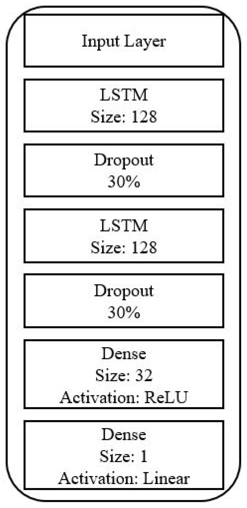
Figure 4 illustrates the architecture of LSTM used in this study, implemented using Keras [29]. The model consists of two LSTM layers to capture temporal dependencies in the data, one dropout layer to prevent overfitting by randomly setting a fraction of input units to 0 at each update during training, and two dense layers in fully connected layers to output the final prediction results.

Figure 4. LSTM architecture diagram [19].

The model’s performance is evaluated using Mean Squared Error (MSE) as the loss function. After each training iteration (i.e., n = 3849), the MSE is calculated and fed back to the NN to adjust the weights of each layer. A smaller MSE indicates higher prediction accuracy, while a larger MSE indicates lower accuracy. The formula for MSE is:

$$\mathrm{M}\mathrm{S}\mathrm{E}={\sum }_{i=1}^n{\left(y-\mathrm{ŷ}\right)}^2/n$$

(11)

where:

-

n is the sample size.

-

y is the actual value.

-

$\mathrm{ŷ}$ is the predicted value.

The model’s predicted stock prices may have small discrepancies from the actual daily stock prices, which can affect the trading points of subsequent trades and the highest and lowest prices during trading. To address this, a correction method [19] is used to adjust the predicted values. While this method reduces prediction error, it only corrects the next day’s predictions and cannot improve future stock price trends.

This study proposes STBC that uses the short-term prediction error of the current day’s stock price to determine if the predicted value needs adjustment and then corrects future stock prices accordingly. Algorithm 1 presents the calibration procedure for calculating the error and determining whether to apply the correction.

Where:

-

R_t is today’s stock price.

-

P_t models today’s predicted stock price.

-

$\delta$ is the calibration threshold.

-

C_last is the previous calibration value.

-

C_t is today’s calibration value.

Algorithm 1. STBC Deviation Calibration Procedure.

1: $P_t=P_t+C_{last}$ 2: $C_t=R_t-P_t$ 3: If $\left|C_t\right|>(R_t\times \delta )$ then 4:  $C_{last}=C_{last}+C_t$ 5: end if

To reduce the prediction error of the model and determine the optimal correction threshold $\mathrm{\delta }$, this study employs GAs to evolve and find the best value. In GAs, the fitness function is used to calculate the fitness value, which evaluates an individual’s adaptability to the environment. The higher the fitness value, the greater the individual’s survival probability. In this study, the fitness value is calculated using the MSE obtained after applying STBC.

Table 2 outlines the parameters and initial values for the GAs. The initial value for the correction threshold is set to 0.05, and the evolution is set to stop after 15 iterations. Given the relatively low complexity of the problem, the Steady State Selection [30] method is used to select individuals for reproduction, which is computationally efficient. After selection, single-point crossover is performed to evolve the next generation, with a mutation rate of 1% during the crossover process. By the end of the GA process, the optimal correction threshold $\mathrm{\delta }$ is identified, which minimizes the prediction error and improves the model’s accuracy.

Table 2. GA parameters.

Parameter	Value/Method
Initial value	0.05
Number of evolutions	15
Selection	Steady State Selection
Mutation rate	1%
Crossover	One-point crossover method

3.4. Trading Strategy

To align with the trading rules and simulated trading conditions in the Taiwan stock market, we define the following buy–sell rules for the simulated trading system.

• Buying is executed on a per-share basis, and selling is also conducted on a per-share basis.
• The transaction fee for each buying or selling action is 1.425‰ of the transaction price.
• A securities transaction tax of 1‰ of the transaction price is levied for each selling action.
• This study does not involve margin trading and short selling and does not consider short covering.
• Selling of stocks is only allowed if the stock is held.
• Simulated trading is conducted in a one-buy-one-sell manner, representing a complete trading cycle. If the last transaction is a buying action, the cost of that purchase is deducted.
• At the end of simulated trading, if the investor still holds stocks, the closing price of the day is used to calculate the final return rate.
• The buying price for each transaction is the model-predicted and corrected highest price of the day, while the selling price is the model-predicted and corrected lowest price of the day.
• A trade is considered unsuccessful if the actual lowest price of the day is not larger than the buying price or the actual highest price of the day is not less than the selling price. If a trade fails on a given day, it is postponed to the next day.
• If two consecutive days of trading fail, the trading activities are halted.
• This study employs 1,000,000 as the total experimental capital for stock trading.

In this study, the investment return rate is used as the evaluation metric for trading strategies and buy–sell strategies. The calculation method for the investment return rate involves subtracting the total cost of purchases from the total revenue from sales, dividing by the total cost of purchases, and finally expressing the result as a percentage. The formula for the return rate is as follows:

$$Investment Return Rate\left(\%\right)={\displaystyle \frac{Total Revenuen from Sales-Total Cost of Purchases}{Total Cost of Purchases}}\times 100$$

(12)

This formula provides a percentage measure of the profit or loss generated from the trading activities relative to the initial investment.

3.5. Genetic Fuzzy System (GFS)

This study uses the K, D, and RSI technical indicators to establish membership functions for Buy (BUY), Sell (SELL), and Hold (HOLD) actions. To identify the optimal parameters for these membership functions, a genetic-evolution-based fuzzy algorithm is employed. This approach aims to enhance the buy–sell strategy by optimizing the parameters of the membership functions through genetic evolution. The pygad package [31] is used to implement the GAs in this study.

The application rules for the K, D, and RSI technical indicators are established to generate BUY, SELL, and HOLD signals based on specific thresholds. These rules help determine the appropriate trading actions according to the current values of the indicators. The rules are as follows:

K—Indicator Application Rules:

-

BUY Signal: If K value ≤ KB_H, then it is a BUY signal.

-

SELL Signal: If K value ≥ KS_L, then it is a SELL signal.

-

HOLD Signal: If KH_L < K value < KH_H, then it is a HOLD signal.

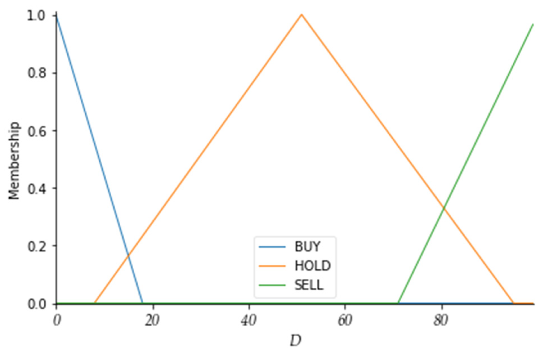
D—Indicator Application Rules:

-

BUY Signal: If D value ≤ DB_H, then it is a BUY signal.

-

SELL Signal: If D value ≥ DS_H, then it is a SELL signal.

-

HOLD Signal: If DH_L < D value < DH_H, then it is a HOLD signal.

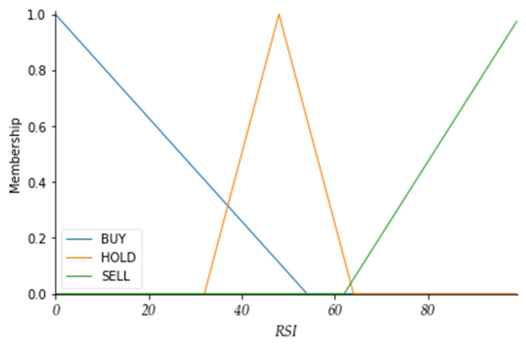
RSI—Indicator Application Rules:

-

BUY Signal: If RSI value ≤ RB_H, then it is a BUY signal.

-

SELL Signal: If RSI value ≥ RS_H, then it is a SELL signal.

-

HOLD Signal: If RH_L < RSI value < RH_H, then it is a HOLD signal.

The rules for each indicator are summarized [32] in Table 3:

Table 3. Rules for technical indicators and signals with action (A.S).

RSI	BUY			HOLD			SELL
K\D	BUY	HOLD	SELL	BUY	HOLD	SELL	BUY	HOLD	SELL
BUY	A.BUY	A.BUY	A.BUY	A.BUY	A.HOLD	A.HOLD	A.BUY	A.SELL	A.SELL
HOLD	A.BUY	A.HOLD	A.BUY	A.HOLD	A.HOLD	A.HOLD	A.SELL	A.HOLD	A.SELL
SELL	A.BUY	A.HOLD	A.BUY	A.HOLD	A.HOLD	A.SELL	A.SELL	A.SELL	A.SELL

Since HOLD indicates no action, we can logically optimize the rules in Table 3 as follows:

• If both K and D indicators signal BUY, then ACTION is A.BUY.
• If both K and D indicators signal SELL, then ACTION is A.SELL.
• If both K and RSI indicators signal BUY, then ACTION is A.BUY.
• If both K and RSI indicators signal SELL, then ACTION is A.SELL.

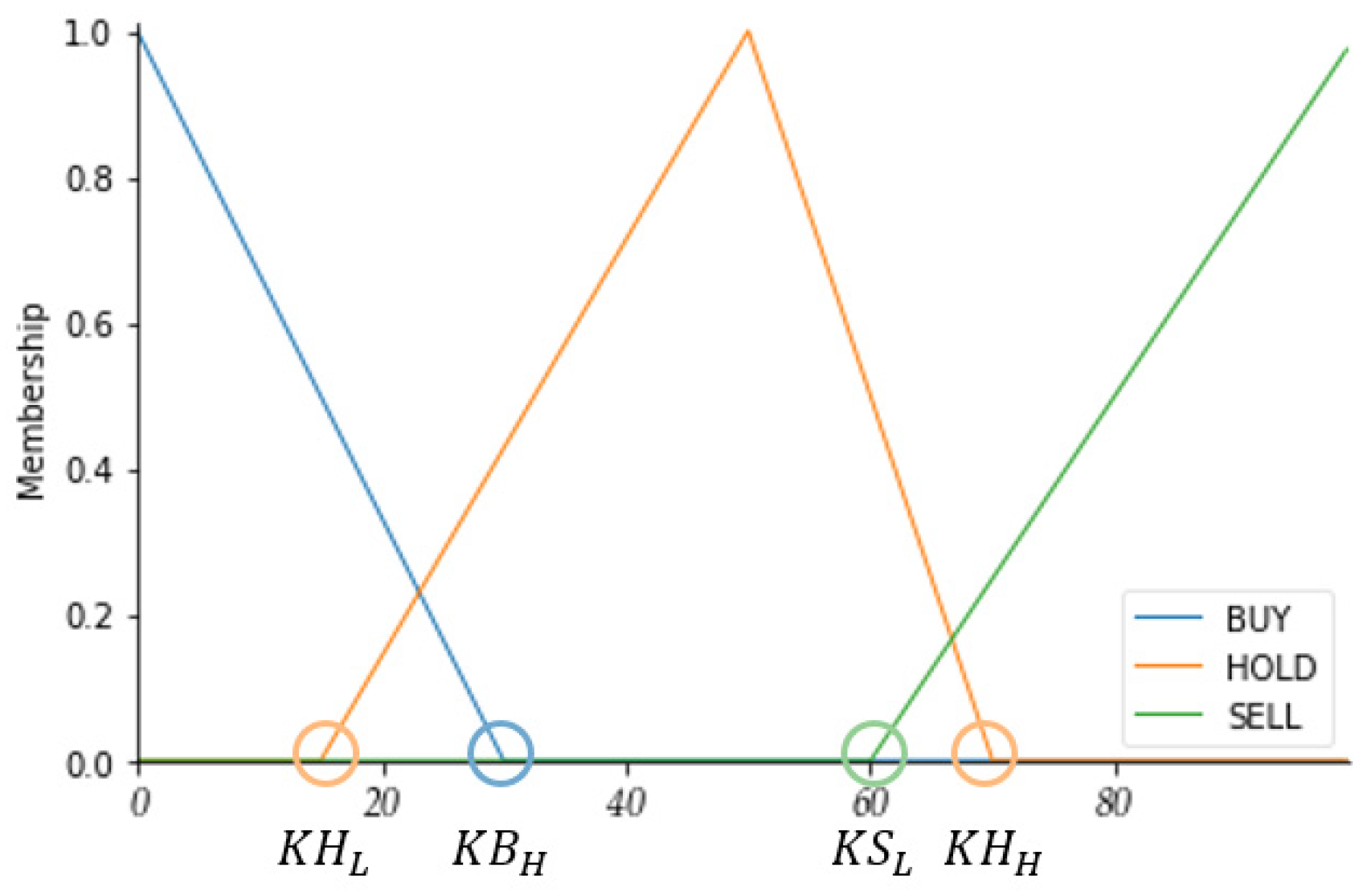
Using the aforementioned technical indicator application rules, we can establish the membership functions as shown in Table 4. This table contains a total of 16 membership function parameters and the corresponding output membership functions.

Table 4. Setting of membership function parameters for technical indicators and outputs.

Indicator\Function	BUY	HOLD	SELL
K	0-0-KBH	KHL-((KHL + KHH)/2)-KHH	KSL-100-100
D	0-0-DBH	DHL-((DHL + DHH)/2)-DHH	DSL-100-100
RSI	0-0-RBH	RHL-((RHL + RHH)/2)-RHH	RSL-100-100
ACTION	0-0-ABH	AHL-((AHL + AHH)/2)-AHH	ASH-100-100

When the K value is less than or equal to KB_H, the ACTION is set to BUY. When the K value is between KH_L and KH_H, it is determined as HOLD. When the K value is greater than or equal to KS_L, the ACTION is set to SELL. This same method of determination is applied to the other indicators, as shown in Figure 5.

Figure 5. Membership functions of K values.

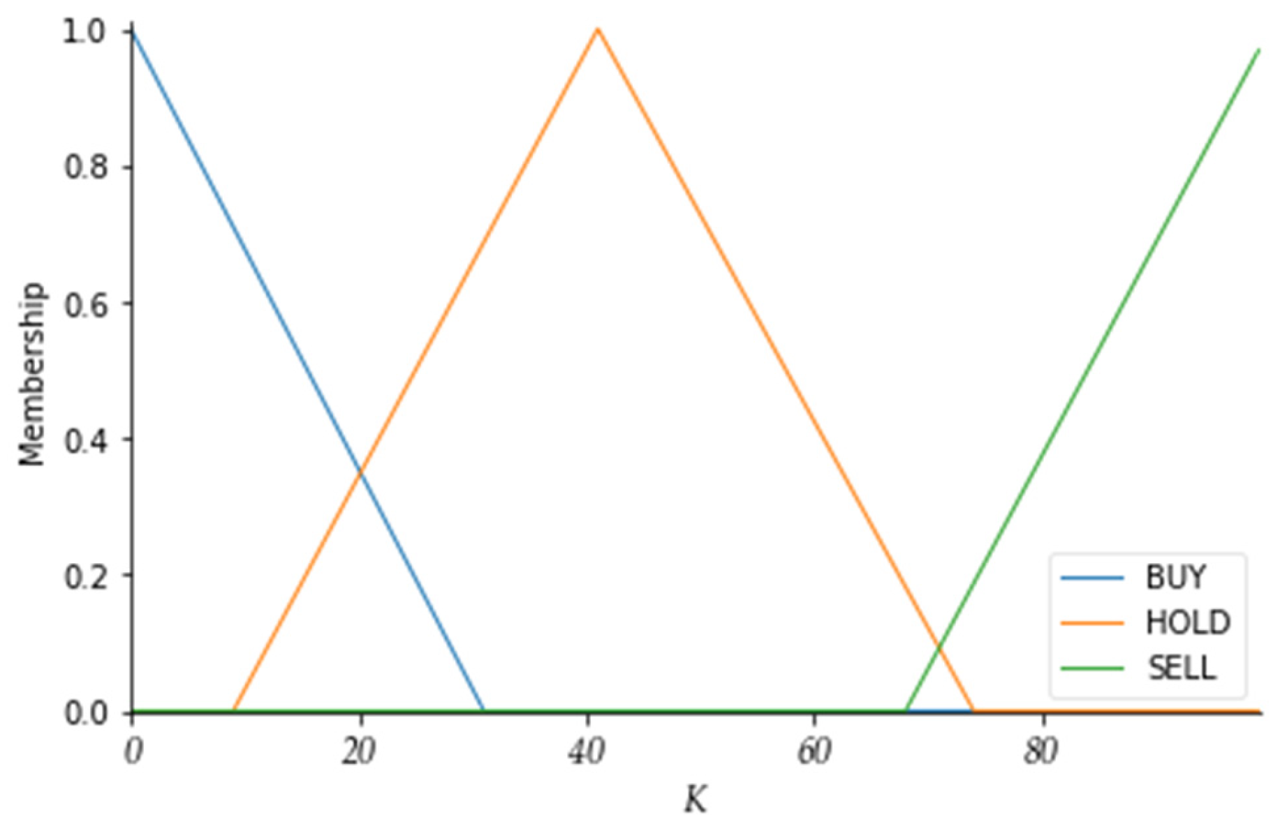
The initial values of the membership functions can be defined based on experience or generated randomly. As shown in Table 5, the K value ranges between 0 and 100. A K value above 80 indicates that the market is overheated and may reverse downwards, which is a signal to sell the stock. A K value below 20 indicates that the market is too cold and may reverse upwards, which is a signal to buy the stock. A K value between 20 and 80 indicates no action. Table 5 shows the initial values of the membership function parameters for the K, D, and RSI indicators.

Table 5. Initial values of membership functions for technical indicators.

Indicator\Function	BUY	HOLD	SELL
K	0-0-20	20-50-80	80-100-100
D	0-0-20	20-50-80	80-100-100
RSI	0-0-30	30-50-70	70-100-100
ACTION	0-0-20	20-50-80	80-100-100

As shown in Table 6, G₁ to G₄ are the parameters for the K indicator membership function, G₅ to G₈ are the parameters for the D indicator membership function, and G₉ to G₁₂ are the parameters for the RSI indicator membership function.

Table 6. GA input variables.

Input Variables of the Genetic Algorithm

G1

G2

G3

G4

G5

G6

G7

G8

G9

G10

G11

G12

Parameters of Membership Functions

KSL

KHL

KHH

KBH

DSL

DHL

DHH

DBH

RSL

RHL

RHH

RBH

The new parameters evolved are input into the membership functions to establish a fuzzy system. The fuzzy system is then used to determine the trading points for buying and selling, and the returns are calculated as the fitness function. This evaluates whether the newly evolved parameters are optimal.

Table 7 shows the training parameters and methods for the genetic fuzzy system. The training evolves for a total of 50 generations, using the Steady State Selection method to select individuals for reproduction. After selection, single-point crossover is used to evolve the next generation, with a mutation rate set at 1%.

Table 7. Training parameters of the genetic fuzzy system.

Parameter	Value/Method
Evolution Rounds	50
Selection Method	Steady State Selection
Mutation Rate	1%
Crossover Method	Single-point Crossover

4. Experimental Results

4.1. Model Prediction

The data for this study were sourced from the Taiwan Stock Exchange, focusing on ETF50 and its largest constituent stock, TSMC. The dataset spans from 30 June 2003 to 31 December 2020. Out of the total data, 90% was used for training and 10% for testing. After excluding null values from the calculation of technical indicators, the final dataset comprised 4297 records. The training data period is from 18 August 2003 to 8 April 2019, while the testing data period is from 9 April 2019 to 31 December 2020.

The MSE of the predicted stock price by the original model is 11.5758, which decreases to 1.2687 after STBC. It successfully reduces the error by nearly 90%, effectively improving future stock price predictions. Figure 6 shows the daily closing prices of the predicted stock prices, while Figure 7 shows the daily closing prices after correction. In the figures, the grey dots represent the actual stock prices of the day and the black dots represent the predicted stock prices. It can be observed that there is a significant deviation between the actual and predicted stock prices during the period marked by the red box, which is from March 2020 to April 2020.

Figure 6. Daily closing prices of model predicted stock prices.

Figure 7. Daily closing prices of corrected model predicted stock prices.

Figure 6 and Figure 7 show that starting from March 2020 (the area marked by the red box), the stock prices show a continuous downward trend. During this time, the model’s predicted stock prices start to deviate from the actual stock prices. Without correction, the future stock price errors could increase, affecting the decision-making process for buying and selling. Through STBC, we can correct the stock prices in a timely manner. For example, on 9 December 2020, the predicted value was 109.53, while the actual stock price of the day was 120.05. There was a deviation between the predicted and actual values. After correction, the adjusted value was 120.39, correcting the error by 10.85, making the prediction more accurate.

To determine the correction threshold in STBC, we used GAs to compute the optimal correction threshold. Table 8 compares the MSE values of STBC with and without the GAs. It can be observed that after obtaining the optimal correction threshold through the GAs, the MSE of the highest price, closing price, and lowest price all decrease. There are three models in the experiment, predicting the highest price, lowest price, and closing price, respectively. To verify whether the predicted stock prices of the three models match the actual stock prices, they are checked after correction. Here, we observe if the lowest price of the day is higher than the highest price. The result shows this situation only occurred on the first day.

Table 8. Comparison of the MSE values of STBC with and without the GAs.

MSE\Method	Original STBC	GA-Optimized STBC
Highest Price (MSE)	1.30058	1.26394
Closing Price (MSE)	1.05160	0.99267
Lowest Price (MSE)	1.21169	1.16202

4.2. Genetic Fuzzy System

After correcting the model predictions, the technical indicator application rules are used to establish a fuzzy system to determine the trading points. To find the optimal membership function values, GAs are used to derive the best parameter values. The parameters of the technical indicator membership functions are input into the GAs for training. Using the parameters derived from the GAs, a fuzzy system is established. By calculating the technical indicators of the stock prices through the fuzzy system, the trading points for buying and selling are determined. Simulated trading is conducted, and the return rate is calculated as the fitness function. After several evolutions, the optimal membership function parameters are obtained.

Table 9 shows that the membership function parameters for the BUY and SELL of the K and D indicators are not significantly different from the initial values. However, there is some difference in the K indicator HOLD membership function parameter KH_L, with the initial value being 20, adjusted to 9 after the GAs. The D indicator follows a similar pattern, with the initial DH_L parameter value being 20, adjusted to 8 after evolution. The RSI indicator BUY membership function parameter RB_H shows a larger difference compared to the initial value of 30. Overall, the 16 parameters, after being trained by the GAs, indeed play a role in optimizing the parameters.

Table 9. Optimal membership function parameters derived from the genetic algorithm.

Input\Function	BUY	HOLD	SELL
K Indicator	0-0-31	9-41-74	68-100-100
D Indicator	0-0-18	8-51-95	71-100-100
RSI Indicator	0-0-54	32-48-64	62-100-100
ACTION	0-0-17	8-51-95	71-100-100

The optimized membership functions, as shown in Figure 8, Figure 9 and Figure 10, result from GA fine-tuning the parameters to achieve the best performance for predicting stock market actions. These functions define the fuzzy logic rules used to determine the appropriate trading actions based on the K, D, and RSI indicators. The training graph of the GAs, showing the relationship between each evolution and the fitness value, indicates that after two evolutions, the fitness value stabilizes around 0.28, with a slight increase.

Figure 8. Optimal membership function of K indicator.

Figure 9. Optimal membership function of D indicator.

Figure 10. Optimal membership function of RSI indicator.

4.3. Comparison of Trading Strategies

Trading strategies determine the appropriate trading points for buying and selling. This study compares three trading strategies: “One-time Conversion” [18], “Fuzzy System (using initial values)”, and “Genetic Fuzzy System”, as shown in Table 10. It can be observed that using the Genetic Fuzzy System achieves a return rate of 32.0%, while the return rates of the other two trading strategies are both less than 5.0%.

$$One-time Conversion Cost={\displaystyle \frac{P_{t+1}-R_t}{R_t}}$$

(13)

where:

-

$P_{t+1}$: Predicted closing price for the next day.

-

$R_t$: Actual closing price of today.

Table 10. Comparison of returns for different trading strategies.

Trading Strategy	Return on Investment (%)
One-time Conversion	4.70
Fuzzy System (using initial values)	4.72
Genetic Fuzzy System	32.00

Table 10. Comparison of returns for different trading strategies.

Trading Strategy	Return on Investment (%)
One-time Conversion	4.70
Fuzzy System (using initial values)	4.72
Genetic Fuzzy System	32.00

4.3.1. Analysis after Price Correction

The test set data start predicting stock prices from 9 April 2019. In the first half of 2020, the COVID-19 event affected the financial market, causing the model’s predicted stock price errors to increase. After correction, as shown by the black dots in Figure 11, the red dots indicate the times when stocks were bought, and the green dots indicate the times when stocks were sold. The period marked by the yellow box is when COVID-19 had the most severe impact on Taiwan.

Figure 11. Impact of COVID-19 on ETF50 stock prices.

It can be observed that despite COVID-19 significantly affecting stock prices, the Genetic Fuzzy System found the optimal buying and selling points. Although there was only one round of trading, the selling point was at an upward trend, which is the desired high point for selling, thus the return rate is relatively high.

4.3.2. Comparison of Returns across the COVID-19 Event

A detailed examination of return performance across different time periods compares the “Buy and Hold” strategy with the GA strategy over a six-month period across the COVID-19 event. The Best Buy and Hold return rate is calculated by buying the stock at the lowest price on the first day and selling it at the highest price on the last day. The Buy and Hold strategy involves buying on the first day and selling on the last day without any transactions in between. Table 11 shows the return rates across the COVID-19 event. In these periods, the Buy and Hold return rates are negative but the Genetic Fuzzy System still yields profits. This indicates that even in challenging market conditions, the Genetic Fuzzy System can achieve stable profits.

Table 11. Comparison of returns across the COVID-19 event.

Time Period	Best Buy and Hold Returns	Buy and Hold Returns	The Proposed Returns
1 July 2019–31 December 2019	18.46	17.30	21.60
1 August 2019–31 January 2020	10.41	9.29	19.76
2 September 2019–27 February 2020	9.61	8.24	9.18
1 October 2019–31 March 2020	−8.96	−11.40	18.02
1 November 2019–30 April 2020	−4.73	−5.10	6.05
2 December 2019–29 May 2020	−7.95	−8.25	0.46
2 January 2020–30 June 2020	−7.31	−7.93	4.29
3 February 2020–31 July 2020	19.06	16.56	19.44
2 March 2020–31 August 2020	20.03	16.54	25.27

5. Conclusions and Future Work

Although stock market trends change rapidly and can cause significant price fluctuations due to various reasons, the STBC proposed in this study can promptly adjust future stock price trends and reduce prediction errors, achieving more accurate stock price predictions. Furthermore, by using fuzzy membership functions optimized through GAs, this study has derived the best parameters for technical indicators, established a fuzzy system, and combined it with technical indicator application rules to infer the best trading points. This approach has been tested through simulated trading, resulting in a positive return rate.

We will further discuss improvements to the correction method and the fuzzy system, outlining two main areas for future enhancement:

Firstly, we can increase the number of technical indicator membership functions and application rules to more accurately determine the best buying and selling points, achieving better results. By introducing more technical indicators, the model’s adaptability to different market conditions can be improved.

Secondly, although STBC can reduce daily prediction errors, frequent corrections might be caused by a few days of significant anomalies, leading to substantial fluctuations in future corrected stock prices. To address this issue, we should limit the correction values to within a reasonable range by using data and errors from previous days to infer the appropriate correction value for future predictions, thus reducing the frequency of corrections. This approach can enhance the model’s stability and accuracy, thereby increasing the return rate.

Finally, while the genetic fuzzy system achieves returns during significant market upswings, its conservative trading strategy limits high profitability. Therefore, we can consider incorporating additional indicators, such as Bollinger Bands, to further optimize entry points and enhance the flexibility and profitability of the trading strategy. These improvements will make the model more stable and effective under various market conditions. The proposed method can also be implicated for other stock markets or financial instruments. It can also contribute to the existing body of knowledge in financial forecasting and machine learning.