Numerical Study on the Lateral Load Response of Offshore Monopile Foundations in Clay: Effect of Slenderness Ratio

Abstract

To meet growing energy demands, offshore wind turbines (OWTs) with higher energy outputs are being developed, presenting increased challenges for their foundation design. Over the past decade, extensive research on the design optimization of OWT support structures has significantly reduced the anticipated costs of offshore wind farm development. Various design methods have been developed and applied in practice, each with its own advantages and limitations. In this study, 3D finite element (FE) modeling, validated against the measured response of a large-scale test monopile, is used to investigate the lateral load response of monopiles with different geometries and slenderness ratios in smaall and large displacements. The results are compared to the standard p–y method, and specific behavioral and design aspects of large-diameter monopiles, such as the moment contribution ratio from different resisting components and the minimum embedment length criteria, are evaluated and discussed. The results showed that the maximum and minimum differences between the 3D FE modeling and one-dimensional (1D) DNV p–y method are 41% and 11% for large displacements, and 32.5% and 13.3% for small displacements, respectively. As the slenderness ratio increases, the discrepancy between the finite element (FE) modeling results and the 1D DNV p–y method decreases, with an average difference of about 13% across all monopile diameters at an L/D ratio of 10, in both small and large displacements, indicating the reasonable accuracy of the 1D method for slenderness ratios of 10 and above. Among the three minimum embedment length criteria examined, the DNV recommended and vertical-tangent criteria offered shorter embedment lengths. The primary resisting moment across all slenderness ratios comes from the distributed lateral load along the monopile shaft (${\mathrm{M}\mathrm{C}\mathrm{R}}_{\mathrm{p}-\mathrm{y}}$), which increases as the L/D ratio increases.

1. Introduction

The development and utilization of renewable energy play a crucial role in achieving “carbon neutrality”. Among the renewable energy sources, offshore wind power has garnered significant attention due to its considerable potential in supporting the energy mix. Offshore wind turbines are supported by various fixed foundation systems such as gravity base foundations, tripod structures, suction caissons, jackets, and monopiles, among which, monopile foundations are currently the most appealing foundation system in moderate water depths of up to 35 m [1]. This mainly stems from their fabrication and installation simplicity, cost-effectiveness, and established logistics [2,3]. Achieving a higher energy output from offshore wind is pursued globally at an ever-increasing pace, which is leading to the design of heavier turbines, taller support structures, and colossal foundation systems. Foundations may account for up to 40% of the total cost of an offshore wind project [4].

Several initiatives were taken to lower the Levelized Cost of Energy (LCOE), which resulted in dropping the tender bid prices for offshore wind farms below the noteworthy threshold of 100 €/MWh from 2015 to 2016 [5]. Such initiatives continue to make offshore wind energy a viable energy source, capable of competing against other forms of energy harvesting. Focus has been allocated to optimizing the design of the support structure, particularly the monopile foundation system, which constitutes a significant portion of the construction costs.

In this regard, current design procedures often adopt the standard p–y method—a simplified one-dimensional (1D) approach—in which the foundation is modeled as an embedded beam. Within this framework, non-linear p–y curves represent the lateral-load–displacement interaction between the soil and the embedded beam. Originally developed for slender piles of a high-embedded-length-(L)-to-diameter (D) ratio (L/D), the standard p–y approach, as proposed by recognized codes (e.g., API RP 2A-WSD and DNVGL-ST-0126 [6,7]), has been widely used in the offshore oil and gas industry [8]. However, significant limitations exist when its application is extended to offshore monopile foundations with relatively small L/D ratios [9,10]. Such limitations stem from the discrepancies between the conditions for which the approach is developed and used.

The p–y approach was developed by studying slender piles with an L/D ratio of about 40 (diameter of 0.32 and embedded length of 12.8 m) for only a few cycles of lateral loading [11]. On the other hand, monopile foundations for offshore wind farm applications are typically designed with significantly lower L/D ratios of around 6 or less and may experience millions of loading cycles in their lifetime [4]. Monopiles experience bending and rotation when loaded laterally, with the balance between the two influenced by the embedment depth and rigidity. Typically, short, embedded piles (with a low L/D ratio) primarily rotate around a center of rotation with minimal bending, while longer, slender piles (with a high L/D ratio) exhibit more bending and a lesser degree of rotation [12]. Due to these behavioral differences, the necessity of establishing tailored design methods for large-diameter, relatively short monopiles is felt to be an alternative to the standard p–y method [13].

Therefore, different research and industrial institutes have allocated efforts to propose improved methods of predicting the lateral response of monopile foundations under different loading and soil conditions, adopting numerical, analytical, and experimental methods. In this regard, large-scale field tests were performed on monopiles in sand, clay, and chalk sites by PISA (Pile Soil Analysis) [10], Li et al., 2017, at Blessington [14], and ALPACA (Axial–Lateral Pile Analysis for Chalk Applying multi-scale field and laboratory testing) [15]. Moreover, centrifuge testing, as a more convenient experimental method, has been performed by the authors in [12,16,17,18,19,20,21,22,23].

Numerical and analytical studies have also contributed to the body of research on the lateral behavior of monopile foundations. In this regard, the pile–soil interaction has commonly been investigated using solid elements for numerical methods [24,25,26,27,28] as well as discrete spring elements for both analytical and numerical methods [8,29,30,31].

The PISA project is one of the most comprehensive studies in this realm, intending to improve the conventional p–y method by incorporating supplementary soil resistance components that are significant for monopiles with a low L/D ratio [32]. Termed as diameter effect, pile tip resistance and interface frictional resistance along the pile surface—as shown in Figure 1—become considerable for large-diameter monopiles with a low L/D ratio [10,33,34,35]. Therefore, the PISA project accounted for the large diameter effect by considering four soil reaction components along the pile, namely, the lateral soil reaction along the shaft (p), the distributed moment reaction due to the vertical shear distribution along the pile (m), the shear force reaction at the pile base ($H_B$) and the moment reaction due to the normal stress distribution at the pile base ($M_B$) [8].

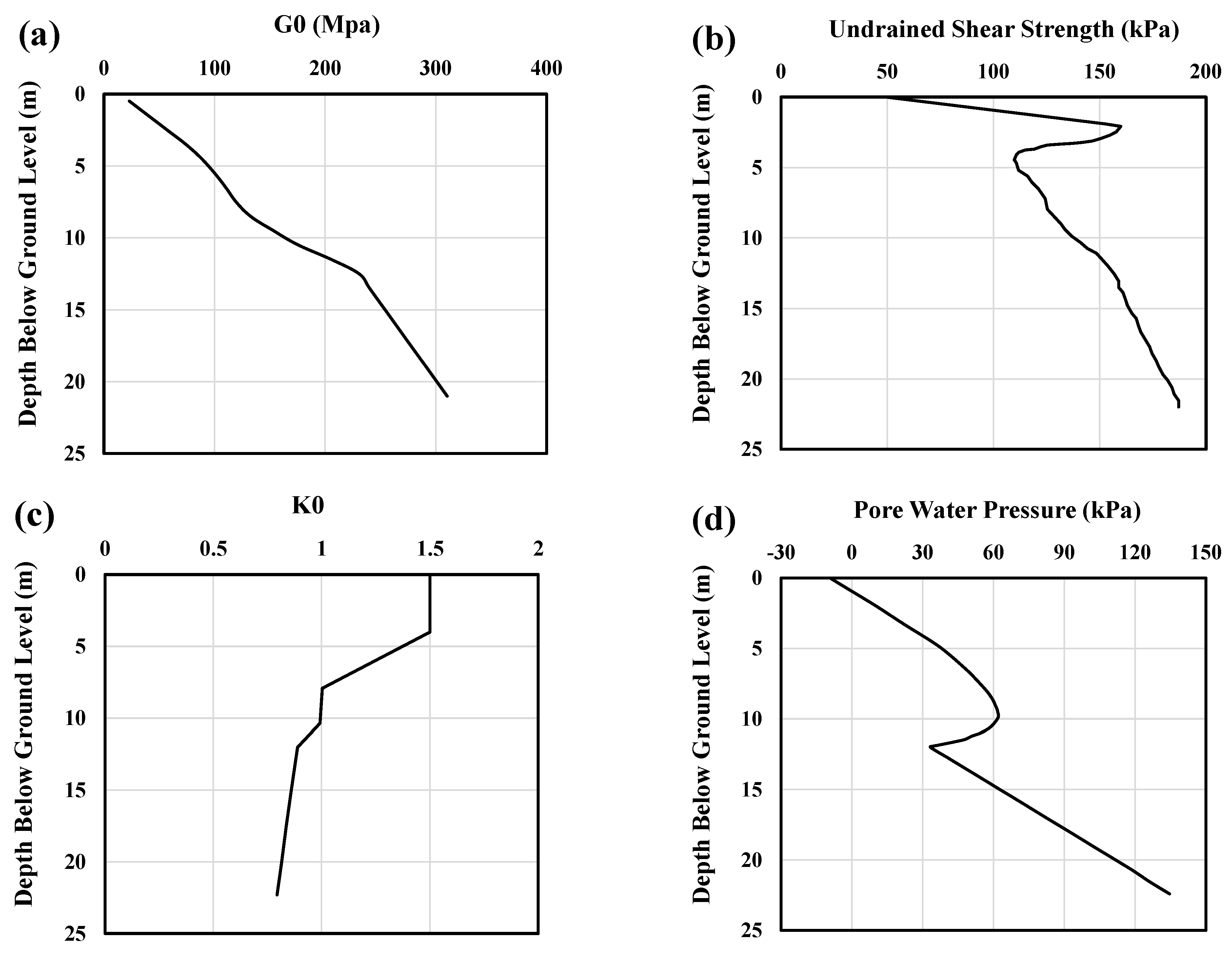
The latest revisions of the DNVGL-ST-0126 guideline suggest that the p–y curves utilized in monopile design should undergo validation via finite element (FE) analysis. Nevertheless, there is currently no consensus on the best method to achieve this in practice [26]. Although previous research has presented different methodologies to conduct such analysis for a wide range of monopile dimensions in homogenous and layered soils, their assumptions should be tested in different offshore site conditions. A literature review reveals that while studies on monopiles in sandy soils or rock-socketed foundations are abundant—reflecting the predominant site conditions in South Korea—few have focused on clay soil profiles in the region. Rigorously validated numerical studies based on large-scale monopile load tests in clay provide a valuable insight into monopile foundation performance, though such studies are limited in the literature. Therefore, more studies are required to develop a comprehensive understanding of the subject and to enrich the database needed to adapt the new design methods. Moreover, simplified one-dimensional methods, as proposed by API and DNV, are still used at the tender design stage and optimization of an entire wind farm, due to their analytical convenience when performing all the necessary design iterations.

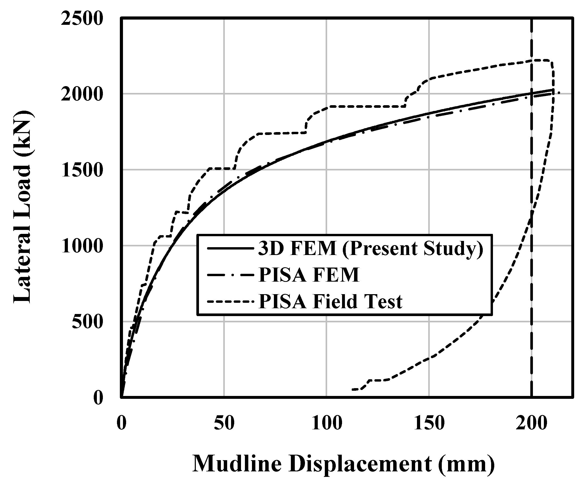
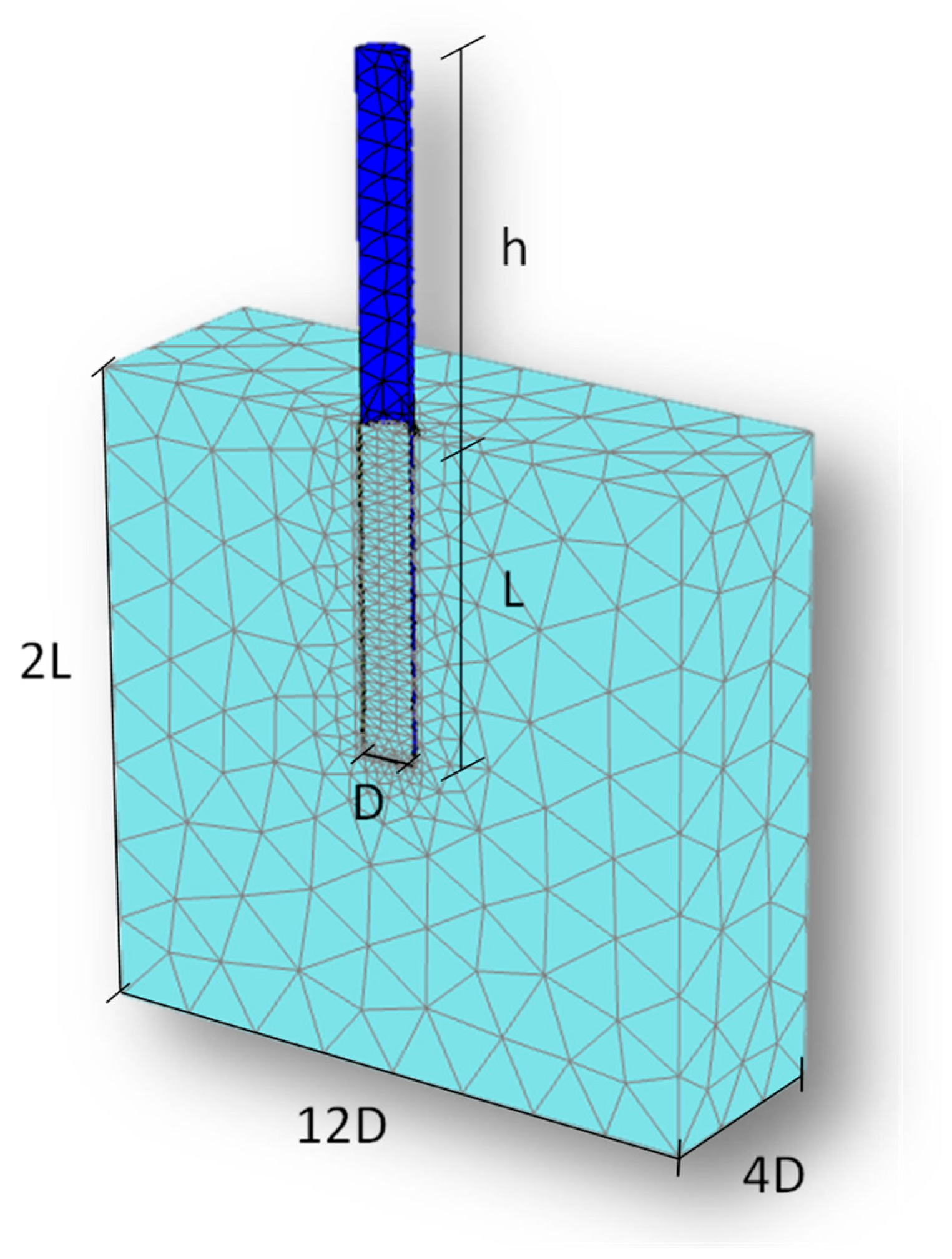
In the present study, the lateral response of monopile foundations in clay has been investigated using 3D numerical modeling and the 1D standard p–y method proposed by common standards. The numerical model has been verified against the results of a large-diameter monopile test conducted by the PISA team at the Cowden site. The 1D standard p–y method, henceforth termed as the 1D DNV p–y method, has been conducted using a commercial finite difference software equipped with the p–y curve formulations suggested by Matlock (1970) and Reese and Welch (1975) for soft and stiff clay, respectively [11,36]. The difference between the predicted lateral response of the monopiles of various geometries using the above-mentioned methods has been evaluated for both small (service) and large (ultimate) displacements. Furthermore, the contribution of different resisting soil components on the lateral capacity of monopiles has been identified for various slenderness ratios, and some design aspects such as the minimum embedment length criteria have been investigated. Finally, several conclusions are drawn, providing factual insights into the shortcomings of the current practice in monopile design, merits offered by numerical modeling, and possible recommendations for improving the current standard p–y method.

2. Finite Element Modeling

To investigate the response of laterally loaded monopiles with varying geometries and slenderness ratios, sixteen 3D numerical models were developed; their geometric characteristics are detailed in

Table 1. Summary of monopile dimensions studied.

No.	Model Code	Dout (m)	L (m)	L/Dout	h (m)	t (mm)
1	D4LD4	4	16	4	40	40
2	D4LD6		24	6		40
3	D4LD8		32	8		40
4	D4LD10		40	10		40
5	D6LD4	6	24	4	40	60
6	D6LD6		36	6		60
7	D6LD8		48	8		60
8	D6LD10		60	10		60
9	D8LD4	8	32	4	40	80
10	D8LD6		48	6		80
11	D8LD8		64	8		80
12	D8LD10		80	10		80
13	D10LD4	10	40	4	40	100
14	D10LD6		60	6		100
15	D10LD8		80	8		100
16	D10LD10		100	10		100

(where t and $D_{out}$ represent the thickness and outer diameter of the monopile). These models utilized displacement-controlled loading, maintaining a constant loading eccentricity (h) of 40 m. The simulations were conducted using the PLAXIS 3D V2024.1.0 finite element program, which is well-suited for handling complex geotechnical structures. PLAXIS 3D features advanced constitutive models that effectively simulate the non-linear and anisotropic behavior of soils.

2.1. Constitutive Model

In this study, an idealized clay soil profile, derived from a real offshore site near the South Korean peninsula, was utilized. The NGI-ADP elastoplastic constitutive model was applied to the clay soil, as described in references [37,38]. This model is specifically designed to capture the anisotropy in the undrained behavior of clays, using a total stress approach. Unlike most constitutive models, the NGI-ADP model allows for the direct input of undrained shear strengths for active (A), direct-simple-shear (D), and passive (P) modes of loading. The NGI-ADP constitutive model has demonstrated decent performance for laterally loaded monopiles in clay soils [39].

Table 2. Parameters of NGI-ADP constitutive model.

Soil Parameter	Description
$\gamma$ ($\mathrm{k}\mathrm{N}/{\mathrm{m}}^3$)	Soil unit weight
$K_0$	Lateral earth pressure coefficient
$S_U^A \left(\mathrm{k}\mathrm{P}\mathrm{a}\right)$	Undrained shear strength
$S_{U,inc}^A (\mathrm{k}\mathrm{P}\mathrm{a}/\mathrm{m})$	Variation in undrained shear strength with depth
$G_{ur}/S_U^A$	Ratio of soil shear modulus to $S_U^A$
$S_U^C/S_U^A$	Ratio of undrained shear strength in triaxial compression to $S_U^A$ (default = 0.99)
$S_U^P/S_U^A$	Ratio of undrained shear strength in triaxial extension to $S_U^A$
$S_U^{DSS}/S_U^A$	Ratio of undrained shear strength in direct simple shear to $S_U^A$
${\tau }_0/S_U^A$	Ratio of Initial in situ maximum shear stress to $S_U^A$
${\gamma }_f^C$ (%)	Ultimate plastic strain for compression
${\gamma }_f^E$ (%)	Ultimate plastic strain for extension
${\gamma }_f^{DSS}$ (%)	Ultimate plastic strain for direct shear

lists the required parameters for the NGI-ADP constitutive model along with their descriptions.

The soil drainage type was set to Undrained (C) to enable a total stress analysis with the direct input of undrained parameters. When simulating laterally loaded monopiles in clay, it is crucial to address the gap created at the interface between the pile and the surrounding soil during loading. For onshore monopiles, where this gap remains dry, the soil’s saturated unit weight should be used. Conversely, for offshore monopiles, where the gap fills with free water, the submerged unit weight should be applied, even in total stress analyses. This approach ensures that the effect of the water-filled gap on counteracting the water pressure on the opposite side of the monopile is included in the modeling. Therefore, the submerged unit weight was used for the soil, with the phreatic level set at the bottom of the model. The clay’s submerged unit weight (γ′) and the lateral earth pressure coefficient K0 were 8.5 kN/m³ and 1, respectively.

The value of ${\tau }_0/S_u^A$ was determined from [38]:

$${\tau }_0/S_u^A=0.5\left(1-K_0\right){\sigma }_{V0}^{\prime }/S_U^A\ge 0$$

(1)

where ${\sigma }_{V0}^{\prime }$ is the initial vertical effective stress, considered positive for compression. The ultimate plastic strains for each layer were calculated as follows [40]:

$${\gamma }_f^C={\gamma }_f^E/2={\gamma }_f^{DSS}/1.5=K_f·S_U^A/G_{ur}·100$$

(2)

where $K_f$ is the calibration parameter and was set equal to 60 [40]. The undrained shear strength ($S_U^A$) was assumed to vary linearly with depth (z) as it is given by (3):

$$S_U^A=5.2+3.1z$$

(3)

To take strength anisotropy into account, the ratios $S_U^P/S_U^A$ and $S_U^{DSS}/S_U^A$ were set to 0.5 and 0.75, respectively [40].

The variation in the small-strain shear modulus of soil, $G_{ur}$, with depth is shown in

Table 3. Variation in small-strain shear modulus of soil with depth for the idealized clay soil profile.

z (m)	${\mathit{G}}_{\mathit{u}\mathit{r}}$ (MPa)
0	14
7	46
20	65
200	177

.

Accordingly,

Table 4. Summary of NGI-ADP constitutive model for the idealized soil profile.

Parameter	Unit	Value
${\gamma }^{\prime }$	$\mathrm{k}\mathrm{N}/{\mathrm{m}}^3$	8.5
$K_0$	-	1
$S_U^A (Z=0)$	$\mathrm{k}\mathrm{P}\mathrm{a}$	5.2
$S_{U,inc}^A$	$\mathrm{k}\mathrm{P}\mathrm{a}/\mathrm{m}$	3.1
$G_{ur}$	$\mathrm{M}\mathrm{P}\mathrm{a}$	Detailed in Table 3
$S_U^C/S_U^A$	-	0.99 (default value)
$S_U^P/S_U^A$	-	0.5
$S_U^{DSS}/S_U^A$	-	0.75
${\tau }_0/S_U^A$	-	0
${\gamma }_f^C$ (%)	%	$60·S_U^A/G_{ur}·100 (K_f=60)$
${\gamma }_f^E$ (%)	%	2·${\gamma }_f^C$
${\gamma }_f^{DSS}$ (%)	%	1.5·${\gamma }_f^C$

lists the summary of the soil parameters for the NGI-ADP model.

For the monopile material, the linear elastic constitutive model was considered, and typical steel properties ($E=210.0 \mathrm{G}\mathrm{P}\mathrm{a} \mathrm{a}\mathrm{n}\mathrm{d} \nu =0.3$) were assigned to it.

2.2. Finite Element Mesh and Boundary Condition

A typical geometry and mesh of the finite element model, along with the respective notations, are illustrated in Figure 2. Due to symmetry, only half of the monopile–soil system is considered in the analysis. The monopile is modeled as an open-ended steel half-pipe with wall thickness (t). To minimize the influence of boundary conditions, the model extends vertically to twice the embedded length of the monopile (2L) and horizontally to 6 times the diameter of the monopile (6D) along the loading direction and 4D perpendicular to it, measured from the monopile centerline [40]. Fixed boundary conditions are applied at the model’s bottom, while normally fixed conditions are applied along its sides. In PLAXIS 3D, the soil and structural plate are discretized using 10-node tetrahedral elements and 6-node triangular elements, respectively. An automated mesh generation procedure in PLAXIS 3D, which considers soil stratigraphy, structural bodies, loads, and boundary conditions, was used to discretize the model.

2.3. Soil–Monopile Interface

An interface between the outer surface of the monopile and the surrounding soil was introduced to model the potential sliding or separation between the two mediums. This interface was represented by joint elements added to the structural plates. To allow for tension cut-off, the Mohr–Coulomb (MC) model was assigned to the interface. The MC stiffness properties were matched to the NGI-ADP parameters of the adjacent soil, while its strength properties, in terms of $S_u$, were adjusted to 65% of the strength of the surrounding soil material.

2.4. Simulation Steps

First, the initial effective stresses are generated using the K0 procedure, considering only the soil elements. The modeling approach is based on undrained soil behavior, in other words, the total stress method. However, the submerged unit weight is used in the calculation of initial stresses because the monopile is offshore, and the smallest gap between the monopile and the surrounding soil will be immediately filled with water. In other words, the presence of free water at the monopile–soil interface means that the effective pressure resisting the lateral movement of the monopile is based on the submerged unit weight.

Subsequently, in phase 1, the predefined steel plate elements that define the monopile geometry and the monopile–soil interfaces are activated, and the model is solved to equilibrium. This phase results in minimal displacement and deformation in the model, which will be reset in the following phase. The assumption that the monopile is “wished in place” is deemed acceptable because the monopile gains its lateral capacity by mobilizing a significant volume of soil around it, extending well beyond the disturbed zone caused by pile installation [28]. Finally, in phase 2, the monopile head is laterally pushed in a displacement-controlled manner until it reaches a lateral displacement of approximately 0.2 times the diameter (D) at the mudline level. This relatively large displacement ensures that the monopile is pushed beyond the displacement required to reach the ultimate limit state. The push is exerted to the center of a rigid top plate, ensuring uniform displacement around the pile perimeter in the loading direction.

2.5. Verification

The numerical model was validated against the results from the CL2 pile test conducted at the Cowden site during the PISA project [41]. The CL2 test monopile had the largest diameter among the tests; its geometric characteristics detailed are

Table 5. CL2 monopile test dimension at Cowden site.

Test	DOUT (m)	L (m)	L/DOUT	h (m)	t (mm)
CL2	2	10.6	5.3	10.1	25

. Initially, a ground profile for the Cowden site was developed using site investigation data and the NGI-ADP constitutive model [27,42]. This ground profile includes approximately 40 m of over-consolidated clay till, underlain by chalk, with the groundwater table 1 m below the surface. The saturated bulk unit weight (${\gamma }_{sat}$) is reported as 21.19 kN/m³. Figure 3 illustrates the variation in the small-strain shear modulus ($G_0$), undrained shear strength in compression ($S_u$), lateral earth pressure coefficient in terms of effective stress ($K_0^{\prime }$), and measured pore water pressures (U) with depth. A detailed description of the ground conditions can be found in the work of Zdravković et al. (2020a) [42].

Since the Cowden site is onshore, the saturated unit weight of the soil was used to generate the initial stresses. Additionally, there is a significant non-linear variation in soil parameters, particularly at near-surface depths, which can affect the accuracy of predicting the response of calibration monopiles. To account for this variation, soil layers with a thickness of 1 m were used to create an appropriate model.

Table 6. Calibration of NGI-ADP constitutive model for Cowden till.

Layer	Top (m)	Bot (m)	${\mathit{K}}_{\mathbf{0}}^{\mathbf{\prime }}$	${\mathit{\gamma }}_{\mathit{s}\mathit{a}\mathit{t}} \mathbf{\left(}\mathbf{k}\mathbf{N}\mathbf{/}{\mathbf{m}}^{\mathbf{3}}\mathbf{\right)}$	U (kPa)	${\mathit{\sigma }}_{\mathit{v}}^{\mathbf{\prime }} \mathbf{\left(}\mathbf{k}\mathbf{P}\mathbf{a}\mathbf{\right)}$	${\mathit{\sigma }}_{\mathit{v}} \mathbf{\left(}\mathbf{k}\mathbf{P}\mathbf{a}\mathbf{\right)}$	${\mathit{K}}_{\mathbf{0}}^{\mathit{t}\mathit{o}\mathit{t}\mathit{a}\mathit{l}}$	${\mathit{S}}_{\mathit{u}}^{\mathit{A}\mathbf{-}\mathit{t}\mathit{o}\mathit{p}} \mathbf{\left(}\mathbf{k}\mathbf{P}\mathbf{a}\mathbf{\right)}$	${\mathit{S}}_{\mathit{u}}^{\mathit{A}-\mathit{b}\mathit{o}\mathit{t}} \mathbf{\left(}\mathbf{k}\mathbf{P}\mathbf{a}\mathbf{\right)}$	${\mathit{S}}_{\mathit{u}}^{\mathit{A}\mathbf{-}\mathit{i}\mathit{n}\mathit{c}} \mathbf{\left(}\mathbf{k}\mathbf{P}\mathbf{a}\mathbf{/}\mathbf{m}\mathbf{\right)}$	${\mathit{S}}_{\mathit{u}}^{\mathit{A}-\mathit{r}\mathit{e}\mathit{f}} \mathbf{\left(}\mathbf{k}\mathbf{P}\mathbf{a}\mathbf{\right)}$	τ0/Su	${\mathit{K}}_{\mathit{f}}$	${\mathit{G}}_{\mathit{u}\mathit{r}}$ (MPa)	${\mathit{G}}_{\mathit{u}\mathit{r}}\mathbf{/}{\mathit{S}}_{\mathit{u}}^{\mathit{A}}$
1	0	1	1.50	21.19	−4.4	15	11	1.500	48.4	104.3	55.9	48.4	0	190	22.9	300.3
2	1	2	1.50	21.19	5.4	26	32	1.415	104.3	160.2	55.9	104.3	0	150	39.9	302.0
3	2	3	1.50	21.19	14.9	38	53	1.359	160.2	149.9	−10.3	160.2	0	120	57.0	367.3
4	3	4	1.50	21.19	24.1	50	74	1.337	149.9	110.0	−39.9	149.9	0	120	74.0	569.1
5	4	5	1.44	21.19	33.5	62	95	1.284	110.0	111.2	1.1	110.0	0	120	88.3	798.1
6	5	6	1.31	21.19	41.4	75	117	1.201	111.2	118.8	7.6	111.2	0	120	99.9	869.3
7	6	7	1.18	21.19	48.4	89	138	1.120	118.8	123.5	4.7	118.8	0	120	110.1	908.8
8	7	8	1.06	21.19	54.2	105	159	1.038	123.5	127.0	3.4	123.5	0	120	119.3	952.9
9	8	9	1.00	21.19	59.1	121	180	1.001	127.0	132.8	5.9	127.0	0	120	132.3	1018.9
10	9	10	1.00	21.19	61.8	140	201	0.998	132.8	138.3	5.5	132.8	0.002	120	153.1	1129.4
11	10	11	0.98	21.19	59.1	163	222	0.989	138.3	146.3	8.0	138.3	0.009	120	175.7	1234.7
12	11	12	0.92	21.19	46.5	197	244	0.936	146.3	154.9	8.6	146.3	0.052	120	205.4	1364.2
13	12	13	0.88	21.19	38.2	227	265	0.901	154.9	158.3	3.4	154.9	0.084	120	230.7	1473.0
14	13	14	0.87	21.19	48.0	238	286	0.895	158.3	161.4	3.1	158.3	0.094	120	240.0	1501.9
15	14	16	0.86	21.19	61.9	256	318	0.891	161.4	167.8	3.2	161.4	0.105	120	254.1	1543.8
16	16	18	0.84	21.19	81.5	279	360	0.877	167.8	174.1	3.2	167.8	0.130	120	272.8	1595.7
17	18	20	0.82	21.19	101.1	301	403	0.868	174.1	181.4	3.6	174.1	0.149	120	291.5	1639.9
18	20	22	0.81	21.19	120.8	324	445	0.859	181.4	187.1	2.9	181.4	0.170	120	310.2	1683.8

lists the calibrated NGI-ADP model parameters for the Cowden site. Given the use of the saturated unit weight for the soil, the lateral pressure coefficient in the middle of each layer was calculated in terms of total stresses as follows:

$$K_0^{total}=(K_0^{\prime }+U/{\sigma }_V^{\prime })/(1+U/{\sigma }_V^{\prime })$$

(4)

The value of ${\tau }_0/S_u^A$ in each layer was determined from (1). The calibration parameter $K_f$ is from [39] and ultimate shear strains were calculated using (2) [39]. Based on triaxial tests performed during the PISA project, the average $S_U^P/S_U^C$ ratio is $0.841$ [27,42] and ratios $S_U^P/S_U^A$ and $S_U^{DSS}/S_U^A$ were calculated as follows:

$$S_U^P/S_U^A=\left(S_U^P/S_U^C\right)\left(S_U^C/S_U^A\right)=0.841\times 0.99=0.833$$

and from [40]:

$$S_U^{DSS}/S_U^A=0.5\times \left(S_U^P/S_U^A+S_U^C/S_U^A\right)=0.5\times \left(0.833+0.99\right)=0.911$$

Figure 4 compares the calculated lateral-load–displacement curve with the observed field behavior from [42]. As can be seen, the calculation results show reasonable agreement with the measured response of the monopile. To assess the accuracy of simulation results compared to field observations, the accuracy metric $\eta$ is defined as follows [27]:

$$\eta =(A_{ref}-A_{diff})/A_{ref}$$

(5)

where $A_{ref}$ is the area below the reference, i.e., field measurements, and $A_{diff}$ is the delimited area between the reference and the simulated curve. Desired $\eta$ values are in the range of 90–100% [40]. The $\eta$ parameter was calculated to be 90%, which indicates acceptable accuracy. Superimposed on the figure is the PISA finite-element-modeling CL2 curve [27], which closely fits the 3D FEM results.

Figure 4. Comparison between the measured and 3D FEM predicted response of CL2 test (PISA field test data from [42], and PISA FEM data fro [27]) [27,42].

Figure 4. Comparison between the measured and 3D FEM predicted response of CL2 test (PISA field test data from [42], and PISA FEM data fro [27]) [27,42].

3. Standard p–y Approach for Monotonic Loads

The behavior of laterally loaded piles is typically analyzed using the p–y method according to the DNVGL-ST-0126 and DNV-RP-C212 guidelines [7,43]. In this approach, the monopile is modeled as a beam with specific properties, connected along its embedded length to multiple springs, whose lateral-load–displacement behavior is defined by p–y curves. These p–y curves represent the ground response through a non-linear relationship between soil resistance and displacement at a given depth. For homogeneous soil conditions, both the ultimate strength ($P_u$) and initial stiffness ($E_{py}$) increase with depth [1]. DNV-RP-C212 recommends different p–y curves for soft and stiff clay [43]. For soft clay, defined as clay with an undrained shear strength up to 100 kPa, Matlock’s (1970) p–y curves are recommended [11]. For stiff clay, defined as clay with an undrained shear strength exceeding 100 kPa, the procedures proposed by Reese et al. (1975) and Reese and Van Impe (2011) are recommended [44,45].

In this regard, Matlock’s (1970) soft-clay p–y curves were used for the upper depth (up to −30.6 m, where the soil’s undrained shear strength ($S_u$) is less than 100 kPa), while Reese and Welch’s (1975) p–y curves for stiff clay were employed at greater depths (beyond −30.6 m, where Su exceeds 100 kPa) [11,36]. Reese and Van Impe (2011) proposed two p–y curve formulations for stiff clay based on whether free water is present (Reese et al. 1975) or absent (Reese and Welch 1975) [36,44,45]. The p–y curve with free water corresponds to the cases where annular scour occurs around the pile during cyclic loading (see Figure 5). Considering that, in the present study, the monopile response under monotonic loading is of interest, the p–y curve without free water proposed by (Welch and Reese 1975) has been adopted for the layers.

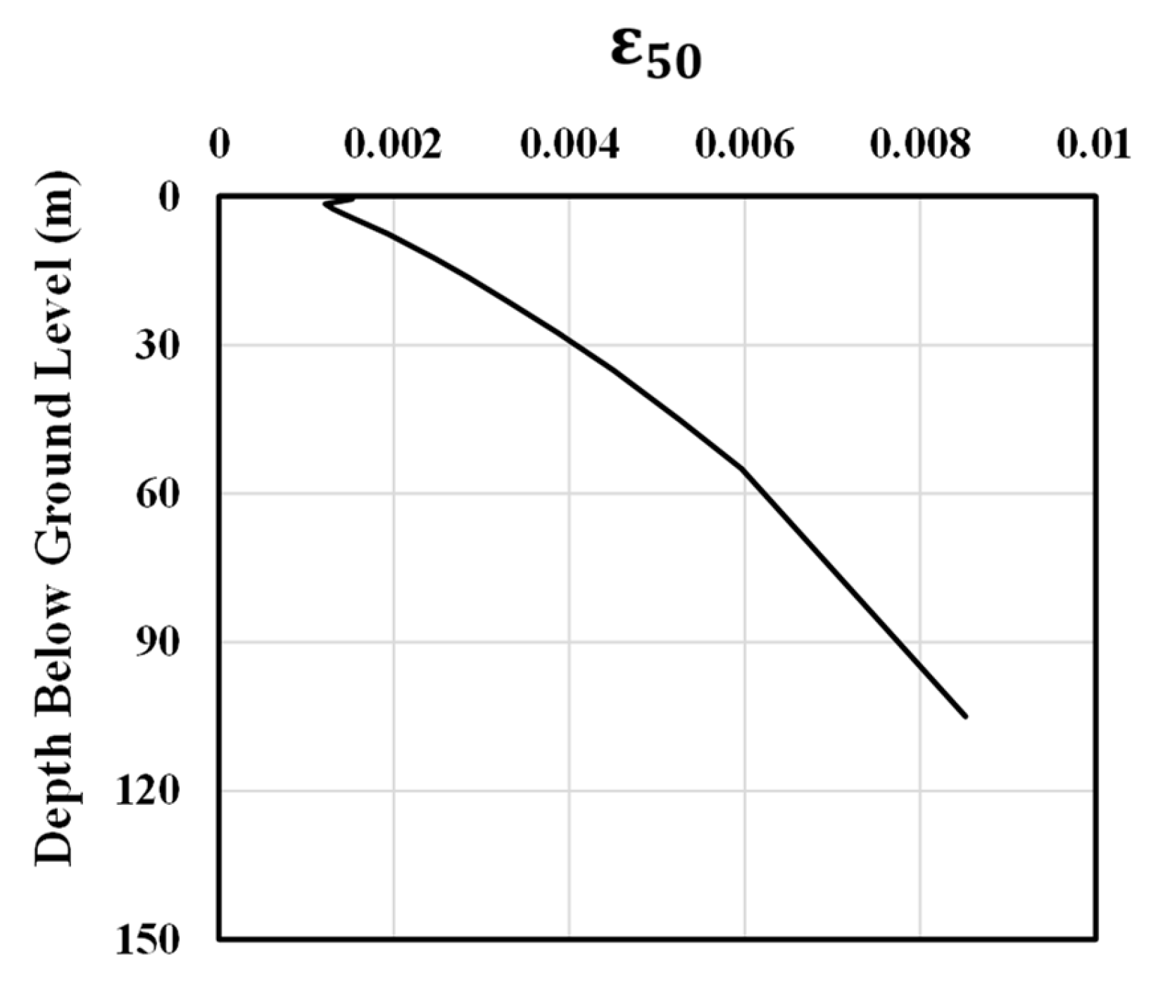
The monopile foundation analysis was performed using the commercial software LPile v2022, which is tailored for evaluating laterally loaded piles via the p–y method. LPile utilizes a finite difference approach to solve the beam–column differential equation, enabling the determination of the deflection, bending moment, shear force, and soil response along the pile’s length. For both the Matlock soft clay and Reese and Welch stiff clay without free water, LPile requires three input parameters: undrained shear strength ($S_u$), effective unit weight (${\gamma }^{\prime }$), and the strain corresponding to half of the maximum difference in principal stresses in the stress–strain curve of the undisturbed specimen of clay (${\mathsf{\epsilon }}_{50}$). The profiles for effective unit weight and undrained shear strength are detailed in Table 4. 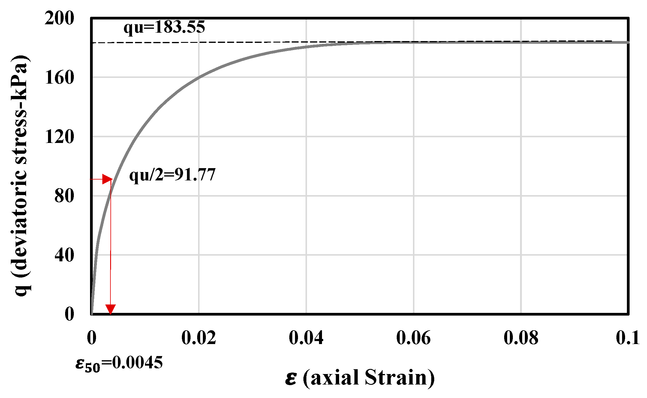To ensure consistency between the two approaches, i.e., the FE and standard p–y methods, ${\mathsf{\epsilon }}_{50}$ values were directly derived from numerical simulations of undrained triaxial tests. PLAXIS software provides a single-element algorithm that allows the simulation of common geotechnical laboratory tests for a defined set of parameters in a given constitutive model. There is no need for meshing in this method, and only the initial stresses on a 3D single element are defined. Then, changes in stress or strain are applied to the element according to the desired test. In this study, a 3-axis compression test was simulated in a displacement-controlled manner to determine ${\epsilon }_{50}$. After applying the initial stresses on a hypothetical element at the desired depth (based on the vertical in-situ stress and the lateral soil pressure coefficient), the axial strain was increased in small steps until the failure of the element (q = qu). Then, the strain corresponding to half of the failure deviatoric stress was determined as ${\epsilon }_{50}$. Figure 6 shows the simulated stress–strain curve for an element at the depth of −35 m. The ${\mathsf{\epsilon }}_{50}$ values used in this study are presented in Figure 7.

4. Results and Discussions

This section examines and discusses the lateral load response of monopile foundations with varying pile geometries based on the results of FE analysis and the 1D DNV p–y method. In the FE model, the load is applied at a height of 40 m above the mudline, while in the 1D DNV p–y analysis, conducted using LPile software, the horizontal load is applied at the mudline, and the load eccentricity is considered by applying an equivalent moment to the monopile at the mudline.

A diameter-to-thickness ratio ($D_{out}/t$) of 100 is maintained across all models in this study. Since the focus is on the lateral behavior of the monopile, no vertical load is considered. DNVGL-ST-0126 states that a criterion on displacement shall be considered as the accepting criterion for adequate lateral pile resistance. Therefore, a displacement of 10% of the monopile diameter is used to define the ultimate lateral capacity and ultimate limit state (ULS) criteria in this study [47]. Additionally, the serviceability limit state (SLS) criterion, based on the same code, is defined as an average rotation of 0.25 degrees at the mudline for a given load applied at an eccentricity above the mudline. The results of this study indicate that this rotation corresponds approximately to a lateral displacement of 1% of the pile diameter at the mudline, for all geometries studied, with a maximum divergence of 5% (see

Table 7. Monopile rotation at 0.01D lateral mudline displacement (in degrees).

L/D	D (m)
	4	6	8	10
4	0.236	0.240	0.242	0.243
6	0.242	0.250	0.254	0.255
8	0.259	0.262	0.265	0.263
10	0.260	0.262	0.254	0.263

). Consequently, for each monopile geometry analyzed, diagrams illustrating both large and small displacements will be presented and discussed. Table 1 details the dimensions studied in this research.

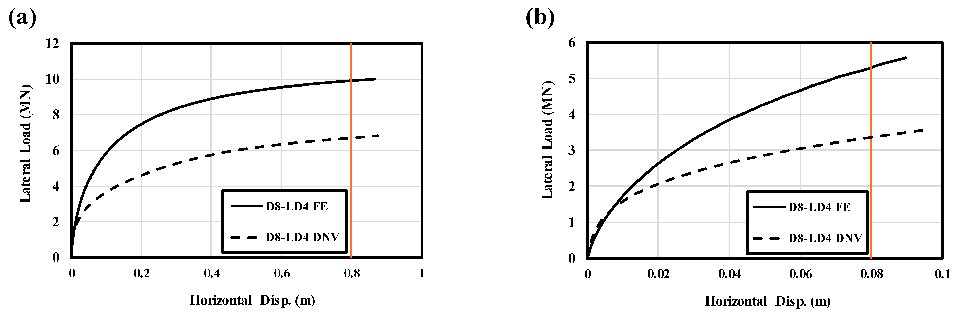
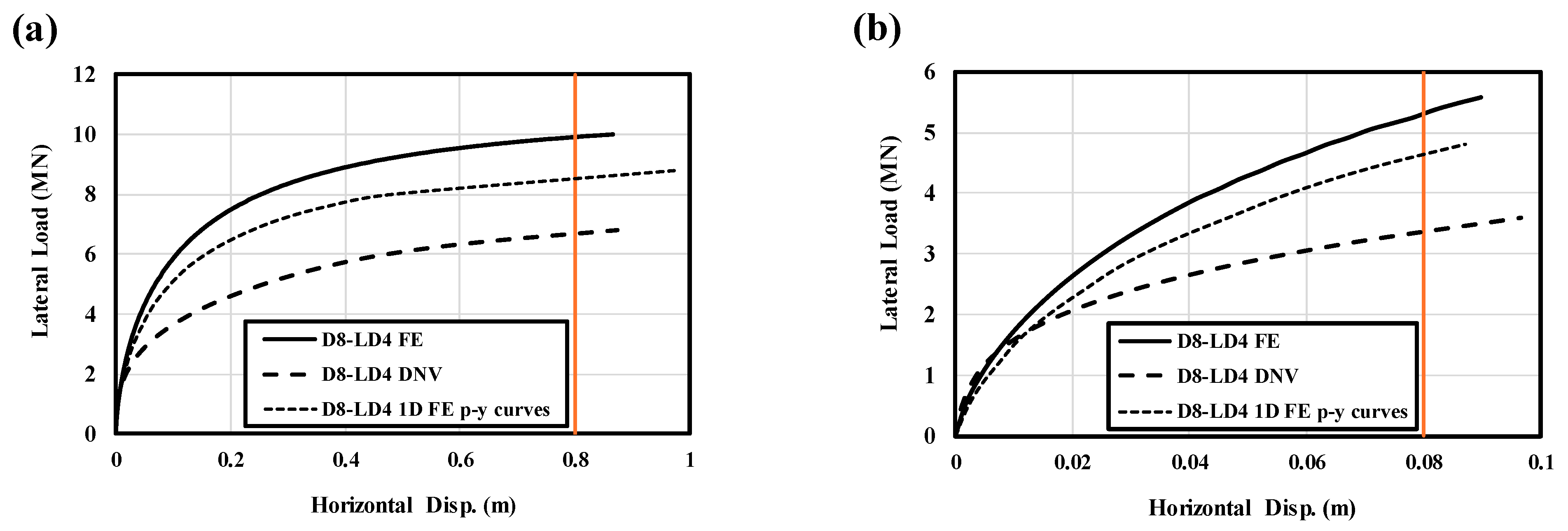
The 8 m monopile serves as the reference diameter in this study. Figure 8 illustrates the load–displacement curves for the D8-LD4 monopile, including results from both the numerical model and the 1D DNV p–y method. As can be seen, the DNV p–y method predicts a lower capacity of the monopile in both small and large displacements. Notably, the difference between the two methods increases with greater pile head displacement. In Figure 8b, it can be observed that at very small displacements (less than 0.02 m), the curves overlap. However, as displacement increases, the difference between the two curves increases, eventually reaching a point where the amount of difference remains nearly constant.

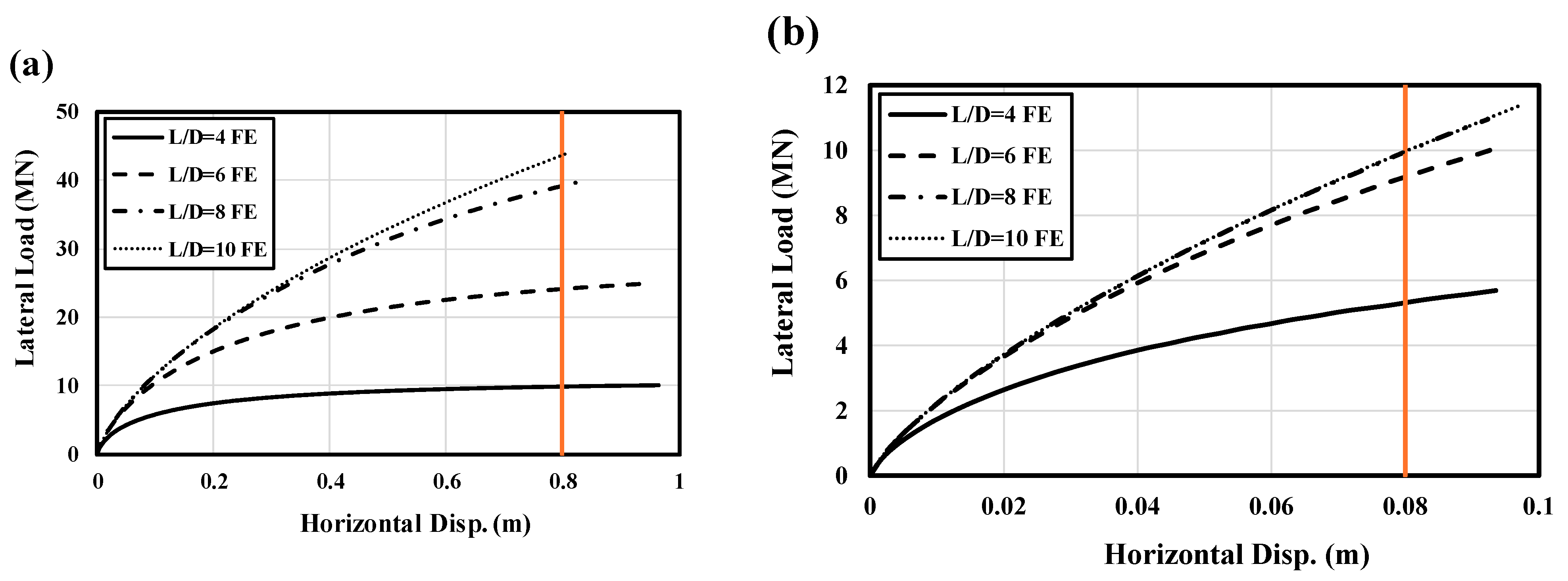
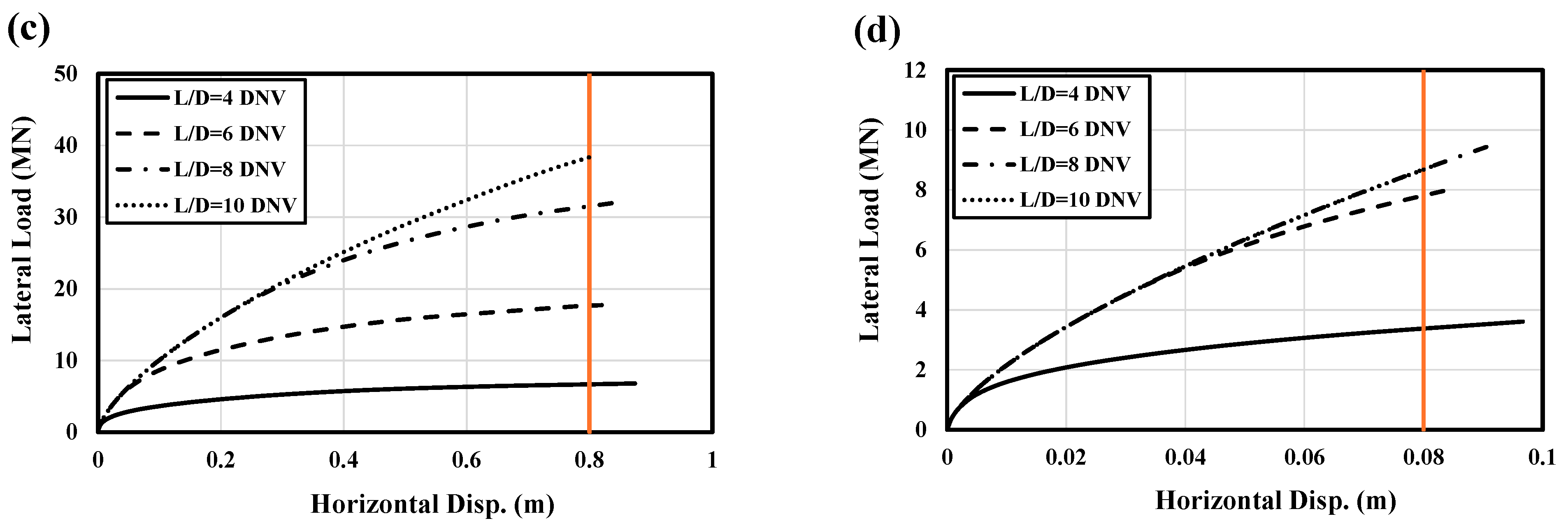
Figure 9 presents the load–displacement results for all L/D ratios considered for the 8 m monopile in this study. Graphs (a) and (b) display the results from the FE model, while graphs (c) and (d) show the results from the 1D DNV p–y method. Figure 9a,c indicate that monopile stiffness and capacity increase with the L/D ratio in both the FE and 1D DNV p–y methods. However, the rate of capacity increase diminishes as the L/D ratio rises. Specifically, the sharp increase observed from an L/D ratio of 4 to 6 turns into a more modest increase from an L/D ratio of 8 to 10.

This trend is more pronounced in small displacements (Figure 9b), where increasing the L/D ratio from 6 to 10 does not significantly enhance capacity. The 1D DNV p–y results, shown in Figure 9c,d, exhibit a similar trend and layout to the FEM results, particularly in the small displacements domain, albeit with a notably weaker load–displacement response.

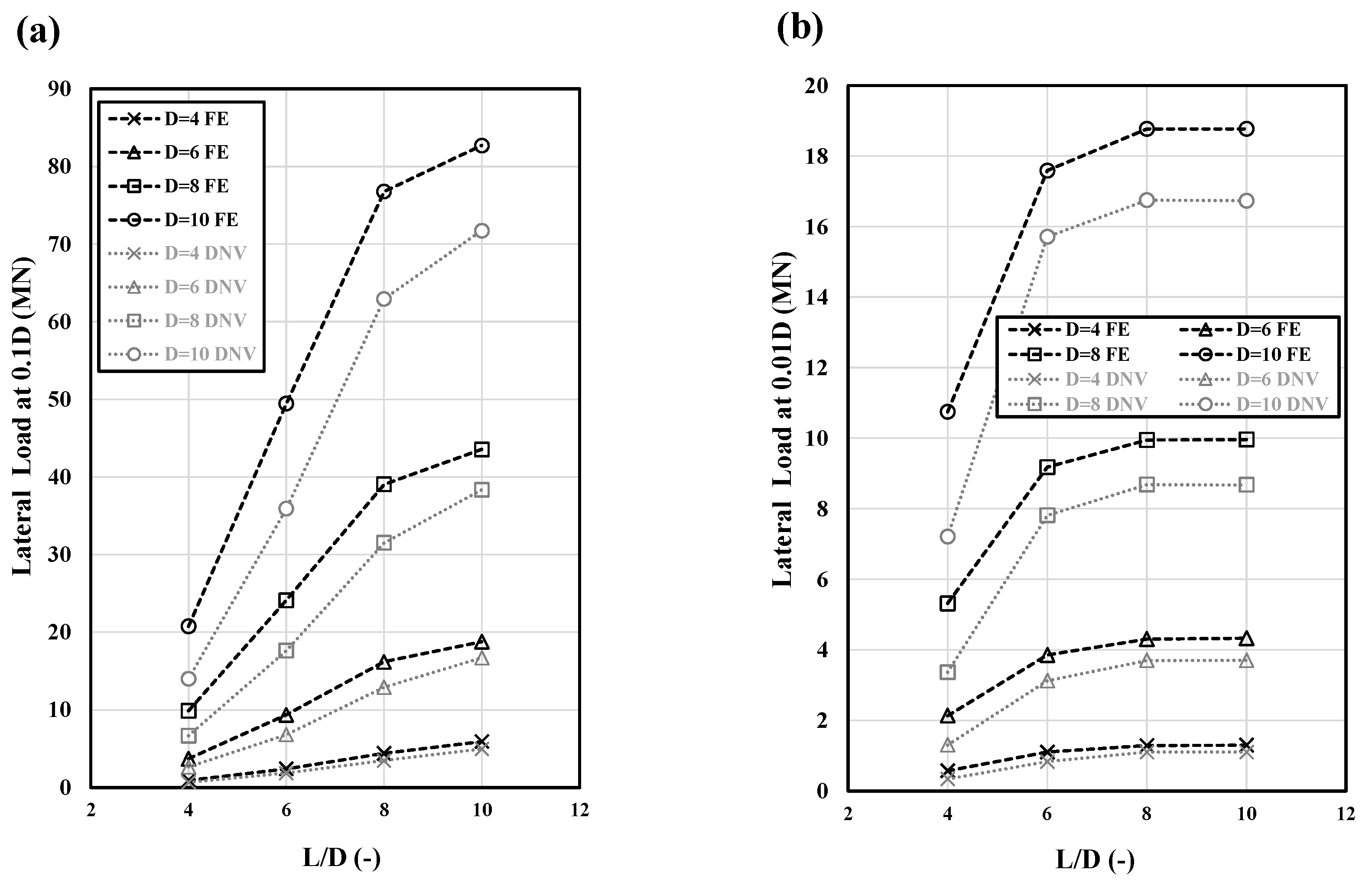
Figure 10 shows the lateral load capacity of all monopile geometries studied in this research at displacements of 0.1D and 0.01D, based on the 1D DNV p–y and 3D FE methods. The results are categorized by small and large displacements for various L/D ratios (4, 6, 8, and 10 m) of the monopile foundations. The findings indicate that while there is a difference in capacity values between the FEM and DNV methods, both show a similar trend of increasing capacity with increasing pile embedment length. As is illustrated in Figure 10a, for large displacements, increasing the embedment length for all monopile diameters leads to a continuous increase in capacity, with the rate of increase declining at an L/D ratio of 8 for both the 1D DNV p–y and 3D FE results. For small displacements, this decline in the rate of increase occurs at an L/D ratio of 6. Beyond this point, further increases in the L/D ratio do not result in significant capacity increases, causing the trend line to stabilize. This suggests that when considering small displacement or service criteria for determining the monopile embedment length, a smaller embedment depth can be selected compared to what would be required for achieving ultimate lateral capacity. Another notable point is the significant effect of increasing the monopile diameter on lateral capacity in both small and large displacements. While this approach can always be considered a viable solution, it is not always the most economical option.

The differences between the results of the 1D DNV p–y and FE methods, as shown in Figure 10, are detailed in Figure 11a,b for large and small displacements in percentages, respectively. According to these graphs, the maximum and minimum percentage differences between the 3D FE and 1D DNV p–y results are 41% and 11% for large displacements, and 32.5% and 13.3% for small displacements, respectively. The results indicate that as the L/D ratio increases, the percentage difference between the FE and 1D DNV p–y results decreases. While this reduction in difference has a steady trendline for small displacements, in large displacements, the rate of reduction decreases as the L/D ratio increases and stabilizes at an L/D ratio of 8 and higher. At an L/D ratio of 10, the discrepancy between the two methods narrows to an average of 13% across all monopile diameters, in large and small displacements. This reduction in the percentage difference with increasing L/D ratio is reasonable, as more slender monopiles align more closely with the conditions for which the DNV p–y method is designed. On the other hand, employing the 1D DNV p–y method for monopiles with an L/D ratio of less than 10 can lead to a substantial underestimation of their lateral capacity, potentially by as much as 41%. It is important to note that these quantities and ratios can vary depending on different soil conditions, the choice of constitutive models, and the specific loading conditions applied.

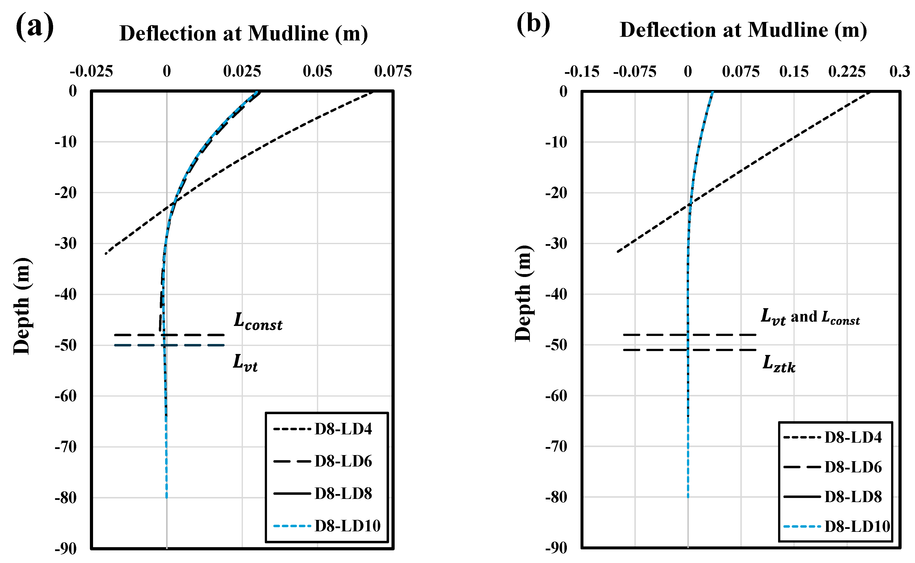
Figure 12a,b display the deflection profiles of the 8 m monopile at various L/D ratios, comparing the FE and 1D DNV p–y analyses, respectively. The deflection is obtained by exerting a 5 MN load at a height of 40 m above the mudline. As the L/D ratio increases from 4 to 10, the deflection at the pile toe decreases to nearly zero for both methods. At an L/D ratio of 4, the deflection profile is nearly linear with a constant slope, indicating rigid rotation with minimal flexure. The FEM results at L/D = 4 show slight flexure, while the DNV results indicate almost no flexure, suggesting nearly rigid behavior. As the L/D ratio increases to 10, the deflection at the pile toe approaches zero, being observed at L/D = 8 in the DNV p–y method and at L/D = 10 in the FEM results. Li et al., 2023, also reported zero deflection at depths of 7 to 9D in their experimental study [12]. For intermediate L/D values, the deflection profiles exhibit a series of curved lines with nonzero values at the end of the pile, indicating a combination of rotation and flexure.

Determining a minimum embedded length to ensure the stability of offshore monopile foundations under severe loading conditions is a crucial step in their design. While various criteria exist for geotechnical monopile design, there is no widely accepted standard for determining the optimal pile length. In many projects, a rigid grip of the pile in the subsoil under significant static loads is essential, which necessitates either a deflection profile with two zero-deflection points (zero-toe-kick criterion, $L_{ztk}$) or at least a vertical tangent (vertical-tangent criterion, $L_{vt}$) [48,49].

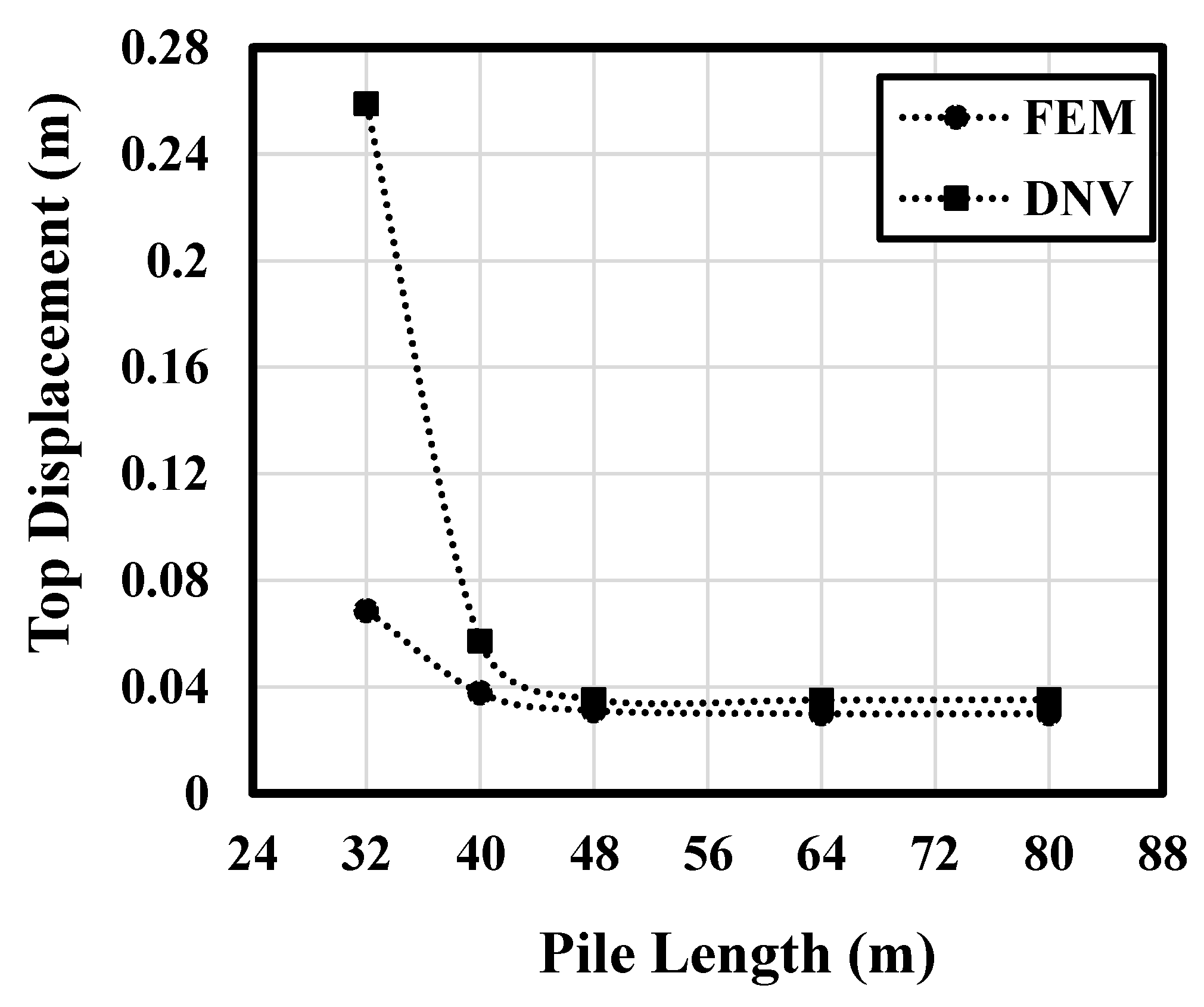
The aforementioned criteria may lead to excessively long embedded pile lengths for large-diameter monopile foundations with significant bending stiffness [50]. As an alternative, DNVGL-2016 proposes analyzing the influence of increased embedded length on pile head displacement and selecting an embedment length that places the design on the “flat part of the corresponding displacement–length curve”. This means that the length ($L_{const}$) should be chosen such that further increases in monopile length have minimal impact on pile head deflection.

Based on the descriptions provided, the critical lengths according to different criteria can be analyzed for both the 1D DNV p–y and FE methods using the data in Figure 12 and Figure 13. According to Figure 13, the $L_{const}$ for both methods is achieved at a pile length of approximately 48 m, beyond which further increases in pile length do not significantly reduce monopile head deflection.

The results also show that the vertical-tangent criterion leads to almost-similar pile lengths, with approximately 48 m for the 1D DNV p–y method and 50 m for the FEM results. Although the vertical-tangent criterion offers embedded lengths similar to the DNV recommendation, previous research has highlighted its unreliability, as this criterion may result in shorter embedded lengths for higher load eccentricities. This is not desirable, as a suitable criterion should lead to a larger pile length for more critical loading conditions [50]. The zero-toe-kick criterion, on the other hand, leads to the longest pile lengths, with approximately 51 m for the 1D DNV p–y method and more than 80 m for the FE results, under the 5 MN load considered.

The response of the monopile using p–y curves extracted from the FE model was also investigated using LPile software. This analysis was conducted for different L/D ratios of the 8 m monopile, the reference diameter in this study. The p–y curves can be extracted from the numerical model, y values through the direct output of the model, and p values from the numerical integration of normal and shear stresses on interface elements. The p–y curves were inserted into the LPile model using the user-defined p–y-curve option. Henceforth, these results will be referred to as the 1D model with FE-extracted p–y curves.

Figure 14 compares the results of the FE analysis, 1D DNV p–y method, and 1D model with FE-extracted p–y curves. It can be seen from Figure 14a,b that in low slenderness ratios (i.e., L/D = 4), there is a clear difference between the results of the FE model and the 1D model with FE-extracted p–y curves for both small and large displacements, highlighting the influence of additional components contributing to the lateral capacity of the monopile. However, as the L/D ratio increases to 6, 8, and 10, the 1D model with FE-extracted p–y curves converges more closely to the FE results. This indicates a reduction in the contribution of other resisting components. At an L/D ratio of 10, the results from the 1D DNV p–y, FE, and 1D model with FE-extracted p–y curves are quite similar, indicating minimal diameter effects for slender monopiles. This demonstrates that for slender piles with an L/D ratio of 10 or higher, the 1D DNV method can predict pile behavior with reasonable accuracy.

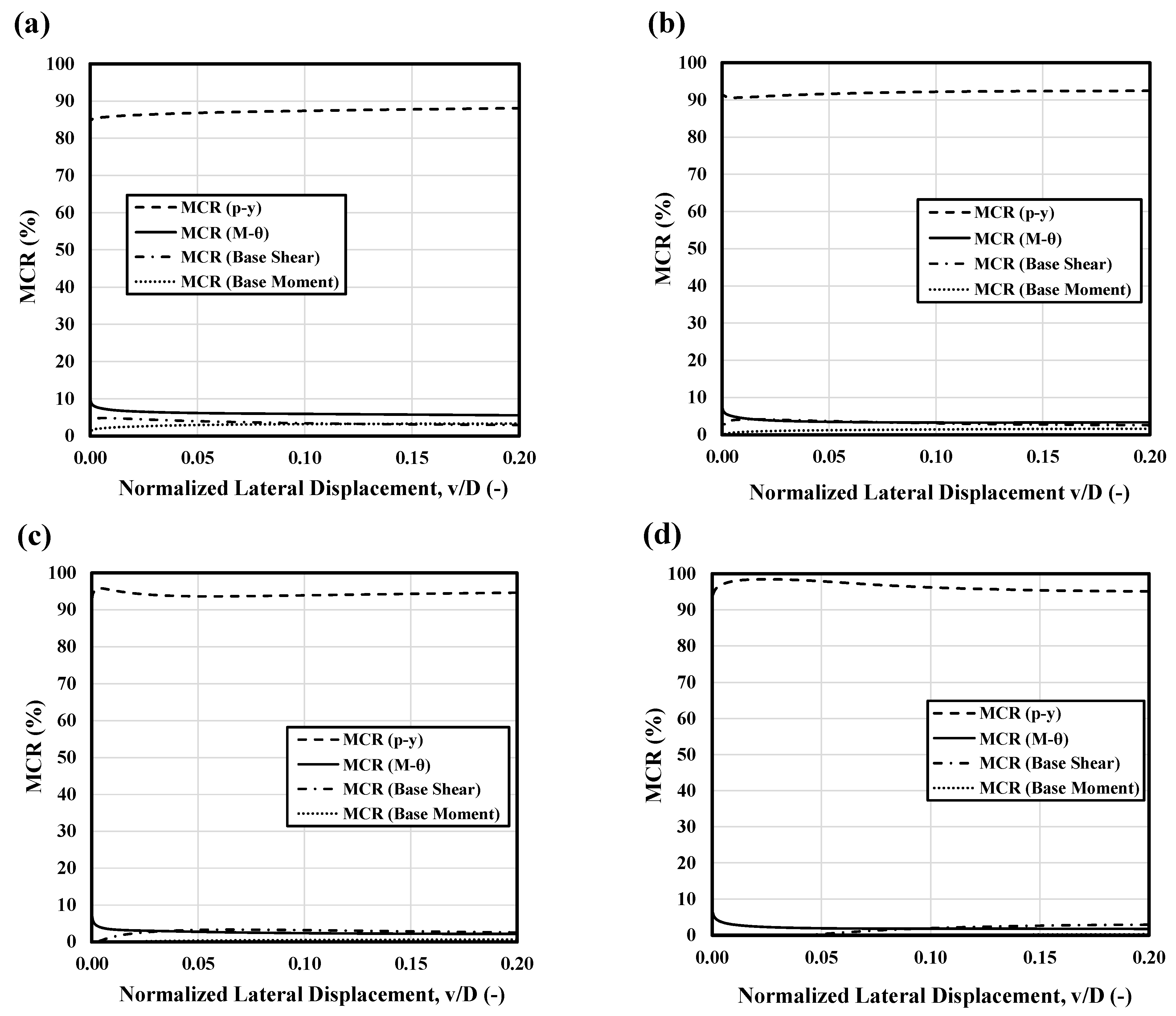
To evaluate the impact of the pile slenderness ratio (L/D) on the relative contribution of the four resisting components, the contribution of each component was expressed as a percentage of the applied moment around the center of rotation (which equals the restoring moment exerted by the soil on the pile). The total moment contribution from the p–y and base shear components (i.e., force components) was determined by multiplying the component force at each depth interval by its distance from the center of rotation (the point of zero lateral displacements, calculated during each load step) and summing these moments for each component. The contribution from the distributed moment caused by vertical shaft shear forces was calculated by integrating the distributed moment, m, along the length of the pile shaft. The total moment from each soil reaction component was then divided by the externally applied moment (applied lateral force × vertical distance to the point of rotation) to calculate the “moment contribution ratio” (MCR). The maximum displacement of 0.2D has been exerted on the monopile, and the displacement of the graphs presented in Figure 15 has been normalized by the diameter of the monopile (D).

The MCR values for each soil reaction component at slenderness ratios of 4, 6, 8, and 10 are presented in Figure 15 for the 8 m monopile. The results indicate that the primary portion of the resisting moment across all slenderness ratios is provided by the distributed lateral load acting along the monopile shaft (${MCR}_{p-\mathrm{y}}$). Furthermore, the contribution of this component increases as the slenderness ratio increases. Specifically, the contribution rises from approximately 87% at an L/D ratio of 4 (Figure 15a) to about 96% at an L/D ratio of 10 (Figure 15d). Conversely, the combined contribution of other components—shear force at the pile base (${MCR}_{BS}$), vertical shear stresses acting on the pile shaft (${MCR}_{M-\mathsf{\theta }}$), and base moment (${MCR}_{BM}$)—decreases as the slenderness ratio increases. At an L/D ratio of 4, these components contribute around 13% (Figure 15a), but their combined contribution drops to 4% at an L/D ratio of 10 (Figure 15d).

The results also revealed that the base moment ${MCR}_{BM}$ minimally contributed to the moment resistance of the monopile with a contribution of around 3 percent at an L/D ratio of 4 and almost zero at an L/D ratio of 10. Except for the L/D ratio of 4 where the vertical shear stresses along the pile shaft, ${MCR}_{M-\mathsf{\theta }}$ have a relatively greater contribution, in other L/D ratios, the ${MCR}_{M-\mathsf{\theta }}$ and ${MCR}_{BS}$ have similar contributions.

5. Conclusions

The lateral load response of monopile foundations in clay was studied using 3D numerical modeling and the 1D standard p–y method from common codes. The model was validated against a large-diameter monopile test by the PISA project team at the Cowden site. The methods were used to evaluate the lateral response of monopiles with different geometries under small (service) and large (ultimate) displacements. The study also identified the contribution of various resisting components to the lateral capacity of monopiles with different slenderness ratios and explored design aspects like minimum embedment length criteria. The main conclusions are summarized as follows:

• The results of the FE and 1D DNV p–y models show that, as the L/D ratio increases for a specific diameter (embedment length increase), the lateral capacity also increases, but the rate diminishes with greater embedment length. This trend is more pronounced at small displacements. For large displacements, increasing embedment length leads to a continuous capacity increase, with the rate declining at an L/D ratio of 8 for both methods. For small displacements, this decline occurs at an L/D ratio of 6, beyond which additional capacity gains are negligible. This suggests that for small displacements or service criteria, a shorter embedment length can be chosen compared to what is needed for ultimate lateral capacity.
• The results showed that among the three minimum embedment length criteria analyzed, the zero-toe-kick criterion led to excessively large embedment lengths. In contrast, the DNV recommended and vertical-tangent criteria provided shorter lengths, with the DNV recommended criterion being the shortest.
• The FE model predicts a higher capacity than the 1D DNV p–y method, particularly at large displacements. This discrepancy arises because of the difference between the distributed lateral reaction on the monopile in the FE model and the p–y curves considered in the 1D DNV p–y method. Additionally, the 1D DNV method does not consider supplementary resisting components such as vertical shaft shear forces, base shear, and the base moment.
• The results showed that the maximum and minimum differences between the 3D FE model and the 1D DNV p–y method were 41% and 11% at large displacements, and 32.5% and 13.3% at small displacements. As the slenderness ratio increases, the difference decreases, averaging 13% at an L/D ratio of 10 across all monopile diameters for both displacement domains. This trend is expected, as a more slender monopile better matches the conditions for which the 1D DNV p–y method is designed. Thus, for L/D ratios of 10 or higher, the 1D method can predict capacity with reasonable accuracy.
• Comparing the 1D DNV p–y method with the 1D FE-extracted p–y curves showed that as the slenderness ratio increased from 4 to 10, the results of the two models converged, reducing the impact of supplementary resisting components. However, the results never fully aligned, highlighting differences in the p–y curves used.
• The primary resisting moment across all slenderness ratios comes from the distributed lateral load along the monopile shaft (${\mathrm{M}\mathrm{C}\mathrm{R}}_{\mathrm{p}-\mathrm{y}}$). This contribution increases with slenderness, rising from about 87% at an L/D ratio of 4 to 96% at an L/D ratio of 10. The results showed that the base moment ${MCR}_{BM}$ minimally contributed to the moment resistance of the monopile, with about 3 percent at an L/D ratio of 4 and nearly zero at an L/D ratio of 10. Except for an L/D of 4, where vertical shear stresses along the pile shaft ${MCR}_{M-\mathsf{\theta }}$ contributed more, ${MCR}_{M-\mathsf{\theta }}$ and base shear ${MCR}_{BS}$ had similar contributions at other L/D ratios.