

Transit Traffic Filtration Algorithm from Cleaned Matched License Plate Data


Abstract
1. Introduction
2. Literature Review
3. Materials and Methods
3.1. Framework for Algorithm Development and Verification
3.2. Transit Traffic Filtration Algorithm
| Algorithm 1 Transit traffic filtration algorithm. |
|
3.3. Verification of the Method
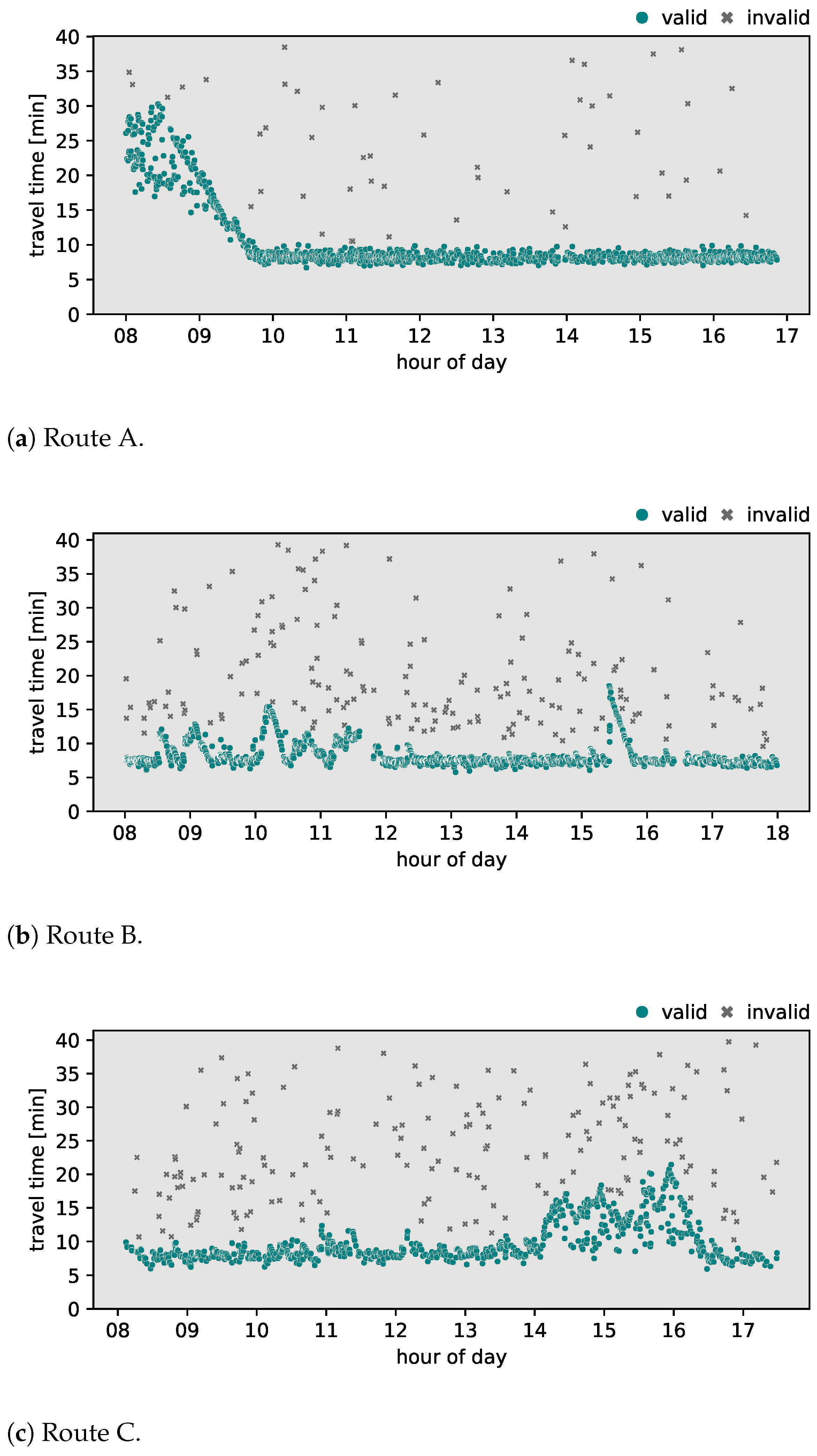
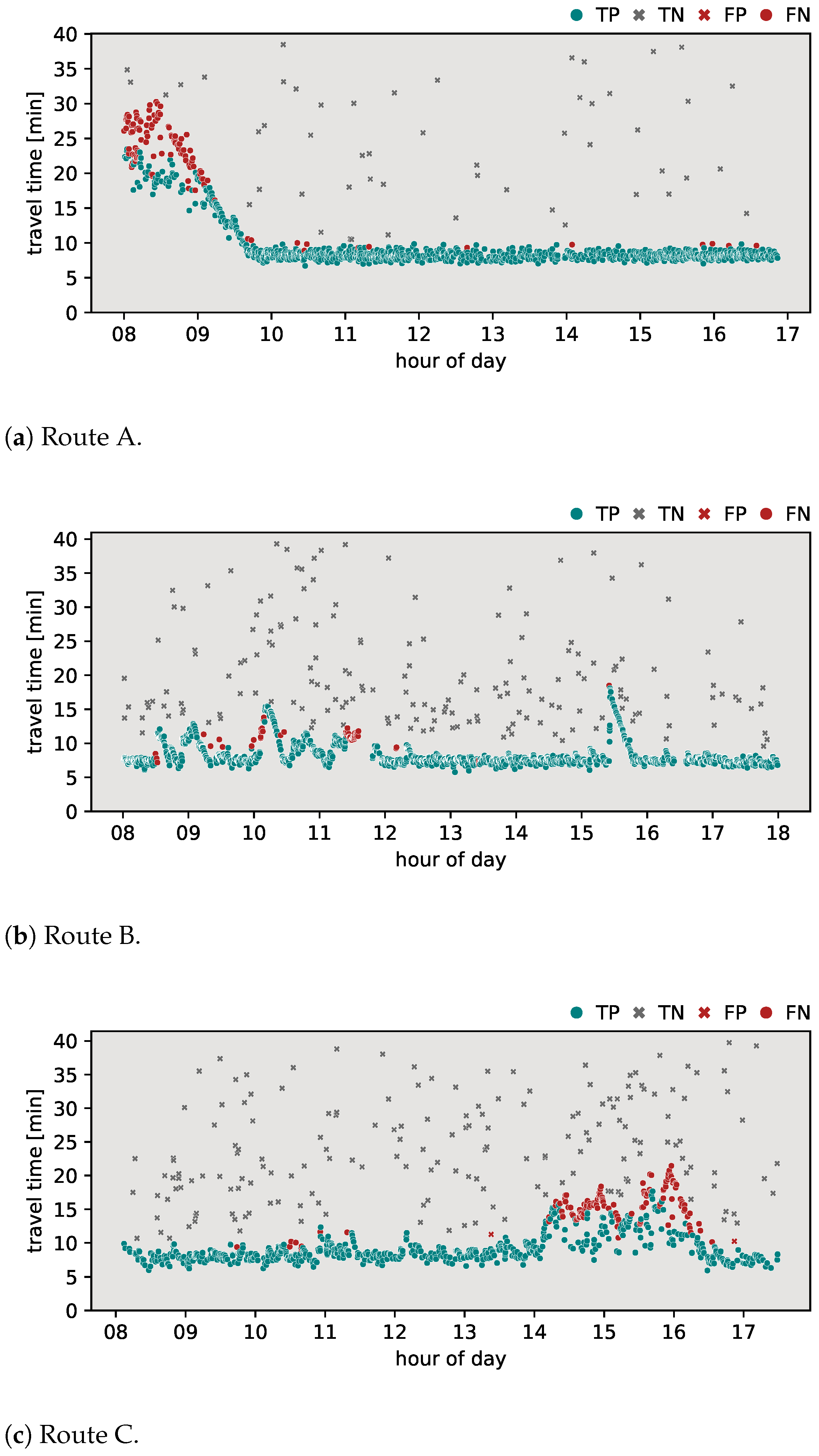
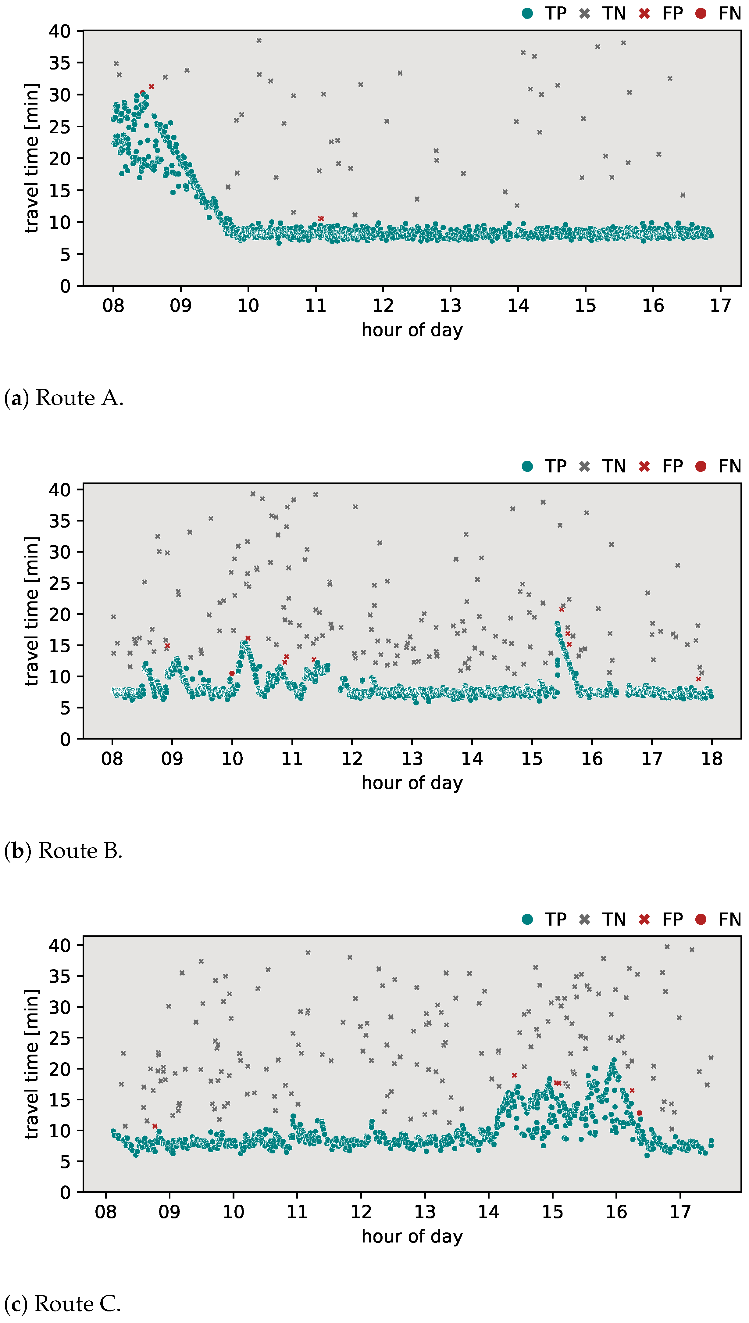
- Route A—urban arterial routeAn important feature of this route is an intersection with a directional ramp that facilitates the transition from a ring road to a main arterial road that enters the city. Other various exits along the route serve nearby residential and commercial areas, allowing vehicles to stop and thus observe non-transit travel times. Furthermore, the presence of a dedicated bus lane plays a key role in influencing travel times along this route, particularly during the morning peak hours. A visual analysis of Figure 2a shows that morning travel times peak at almost 30 min, reflecting the impact of capacity limitations due to infrastructure characteristics. After the morning rush hour, around 10 A.M., travel times stabilize at approximately 9 min, translating to an average speed of around 65 km per hour. The above-mentioned behavior can be seen on a graphical representation of the travel times plot during the morning rush hour.
- Route B—suburban commute routeCharacterized by a two-lane configuration with a single lane in each direction, overtaking is generally prohibited in most sections of this route. Two villages along the way with several pedestrian crossings contribute to reduced speeds. A notable feature is a single-lane roundabout with relatively high traffic flow, which could influence travel times along the route. In the visual examination presented in Figure 2b, morning travel times exhibit fluctuations ranging between 8 and 15 min, with sporadic data gaps during certain time periods. In the afternoon, a notable traffic accident occurred on this route, leading to longer travel times of up to 20 min. After the accident, travel times stabilize around 8 min in the afternoon, corresponding to an average speed of approximately 56 km per hour. This observation underscores the impact of external factors, such as accidents, on the temporal dynamics of travel times along route B.
- Route C—urban transit routeRoute C is characterized as a transit route through the city, featuring multiple intersections and notable points of interest, such as commercial and residential areas, along with the city center. A visual analysis of Figure 2c shows a relatively stable but oscillating pattern of travel times throughout the day. This minor variability can be attributed to the transit nature of the route, influenced by several major intersections that affect travel times. During the afternoon period, a more pronounced fluctuation is evident, particularly during rush hour. Some vehicles appear to have taken faster paths along this route, resulting in lower observed travel times compared to vehicles that followed the conventional path. Given that the route traverses the entire city, there are instances of non-transit vehicle travel times, which could reflect partial destinations within the city during their overall journey. Stable travel times along this route are consistently around 9 min, resulting in an average speed of 37 km per hour.
4. Results
5. Discussion
6. Conclusions
Author Contributions
Funding
Institutional Review Board Statement
Informed Consent Statement
Data Availability Statement
Conflicts of Interest
References
- Qi, W.; Rao, B.; Fu, C. A Novel Filtering Method of Travel-Time Outliers Extracted from Large-Scale Traffic Checkpoint Data. J. Transp. Eng. Part Syst. 2024, 150. [Google Scholar] [CrossRef]
- Nadrian, H.; Heizomi, H.; Shirzadi, S.; Moradi, M.S.; Hajibadali, P. Exploring the dimensions of urban quality of life associated with urban traffic jam: The development and validation of an instrument. J. Transp. Health 2022, 26, 101463. [Google Scholar] [CrossRef]
- Cats, O.; West, J.; Eliasson, J. A dynamic stochastic model for evaluating congestion and crowding effects in transit systems. Transp. Res. Part Methodol. 2016, 89, 43–57. [Google Scholar] [CrossRef]
- Fowkes, A.S. The Use of Number Plate Matching For Vehicle Travel Time Estimation. In Proceedings of the Seminar, Developing Countries, the PTRC Annual Summer Meeting, University of Warwick, Coventry, UK, 4–7 July 1983; p. 240. [Google Scholar]
- Montgomery, F.; May, A. Fators Affecting Travel Times on Urban Radial Routes. Traffic Eng. Control 1987, 28, 452–458. [Google Scholar]
- Clark, S.D.; Grant-Muller, S.; Chen, H. Cleaning of Matched License Plate Data. Transp. Res. Rec. 2002, 1804, 1–7. [Google Scholar] [CrossRef]
- Robinson, S.; Polak, J. Overtaking rule method for the cleaning of matched license-plate data. J. Transp. Eng. 2006, 132, 609–617. [Google Scholar] [CrossRef]
- Dion, F.; Rakha, H. Estimating dynamic roadway travel times using automatic vehicle identification data for low sampling rates. Transp. Res. Part Methodol. 2006, 40, 745–766. [Google Scholar] [CrossRef]
- Houston TranStar—About Houston TranStar. Available online: https://www.houstontranstar.org/about_transtar/ (accessed on 15 August 2023).
- Southwest Research Institute. Automated Vehicle Identification Model Deployment Initiative System Design Document; Technical Report SwRI Project No. 10-8684; Southwest Research Institute: San Antonio, TX, USA, 1998. [Google Scholar]
- Mouskos, K.C.; Niver, E.; Pignataro, L.J.; Lee, S.W.; Antoniou, N.; Papadoupolos, L. Transmit System Evaluation; Final Report; New Jersey Institute of Technology: Newark, NJ, USA, 1998. [Google Scholar]
- Zheng, P.; McDonald, M. Estimation of travel time using fuzzy clustering method. IET Intell. Transp. Syst. 2009, 3, 77–86. [Google Scholar] [CrossRef]
- Bezdek, J.C. Pattern Recognition with Fuzzy Objective Function Algorithms; Springer US: Boston, MA, USA, 1981. [Google Scholar] [CrossRef]
- Moghaddam, S.; Hellinga, B. Algorithm for detecting outliers in Bluetooth data in real time. Transp. Res. Rec. 2014, 2442, 129–139. [Google Scholar] [CrossRef]
- Jang, J. Outlier filtering algorithm for travel time estimation using dedicated short-range communications probes on rural highways. IET Intell. Transp. Syst. 2016, 10, 453–460. [Google Scholar] [CrossRef]
- Asqool, O.; Koting, S.; Saifizul, A. Evaluation of outlier filtering algorithms for accurate travel time measurement incorporating lane-splitting situations. Sustainability 2021, 13, 3851. [Google Scholar] [CrossRef]
- Li, J.; Van Zuylen, H.; Deng, Y.; Zhou, Y. Urban travel time data cleaning and analysis for Automatic Number Plate Recognition. Transportation Res. Procedia 2020, 47, 712–719. [Google Scholar] [CrossRef]


| Algorithm | Assumptions | Advantages | Disadvantages |
|---|---|---|---|
| Percentile | 20% of observations classified as outliers | Simple and easy to use | Algorithm incorrectly classifies 20% of data as outliers without regard to their validity |
| Mean absolute deviation | Observations are classified as outliers if they fall outside a validity range of 3 MAD | Simple and easy to use | Algorithm classifies all values outside the validity range as outliers without regard to their validity |
| Dion, Rakha algorithm [8] | Algorithm uses time intervals; validity range is based on observations in previous time interval | Takes into account the relationship between neighboring time intervals | Hard to apply, high number of user-defined parameters, does not react to abrupt changes in travel times |
| Robinson and Polak [7] | Vehicles with valid travel time observation will tend not to be overtaken, and if on multilane road then travel times will not be greatly dissimilar to overtaking vehicles | Simple and easy to use | Depends on tolerance time parameter, which can be obtained from known distribution of valid travel times |
| Jang algorithm [15] | Algorithm uses time intervals; validity range is based on observations in previous time interval | Takes into consideration the relationship between neighboring time intervals, could tract abrupt changes | Hard to calibrate due to a large number of user-defined parameters |
| License Plate | Entry Time | Exit Time | Travel Time (s) |
|---|---|---|---|
| 5AP***9 | 08:35:09 | 08:46:03 | 654 |
| 3AY***0 | 08:35:16 | 08:46:11 | 655 |
| 6M6***1 | 08:35:18 | 08:46:15 | 657 |
| 8U9***9 | 08:35:24 | 17:08:24 | 30,780 |
| 6E3***9 | 08:35:27 | 08:46:17 | 650 |
| 5H1***1 | 08:36:04 | 08:46:30 | 626 |
| 4M7***8 | 08:36:06 | 08:46:35 | 629 |
| 6P6***1 | 08:36:07 | 08:46:38 | 631 |
| 2H7***4 | 08:36:08 | 08:46:40 | 632 |
| 2H3***8 | 08:36:11 | 08:46:44 | 633 |
| 5H5***2 | 08:36:19 | 08:47:10 | 651 |
| 3SD***8 | 08:36:21 | 08:47:14 | 653 |
| 5E6***1 | 08:36:39 | 08:47:16 | 637 |
| 6E0***7 | 08:36:41 | 08:47:20 | 639 |
| 3AU***2 | 08:36:42 | 08:47:22 | 640 |
| Route | Algorithm | True Positives | False Positives | False Negatives | True Negatives | -Score |
|---|---|---|---|---|---|---|
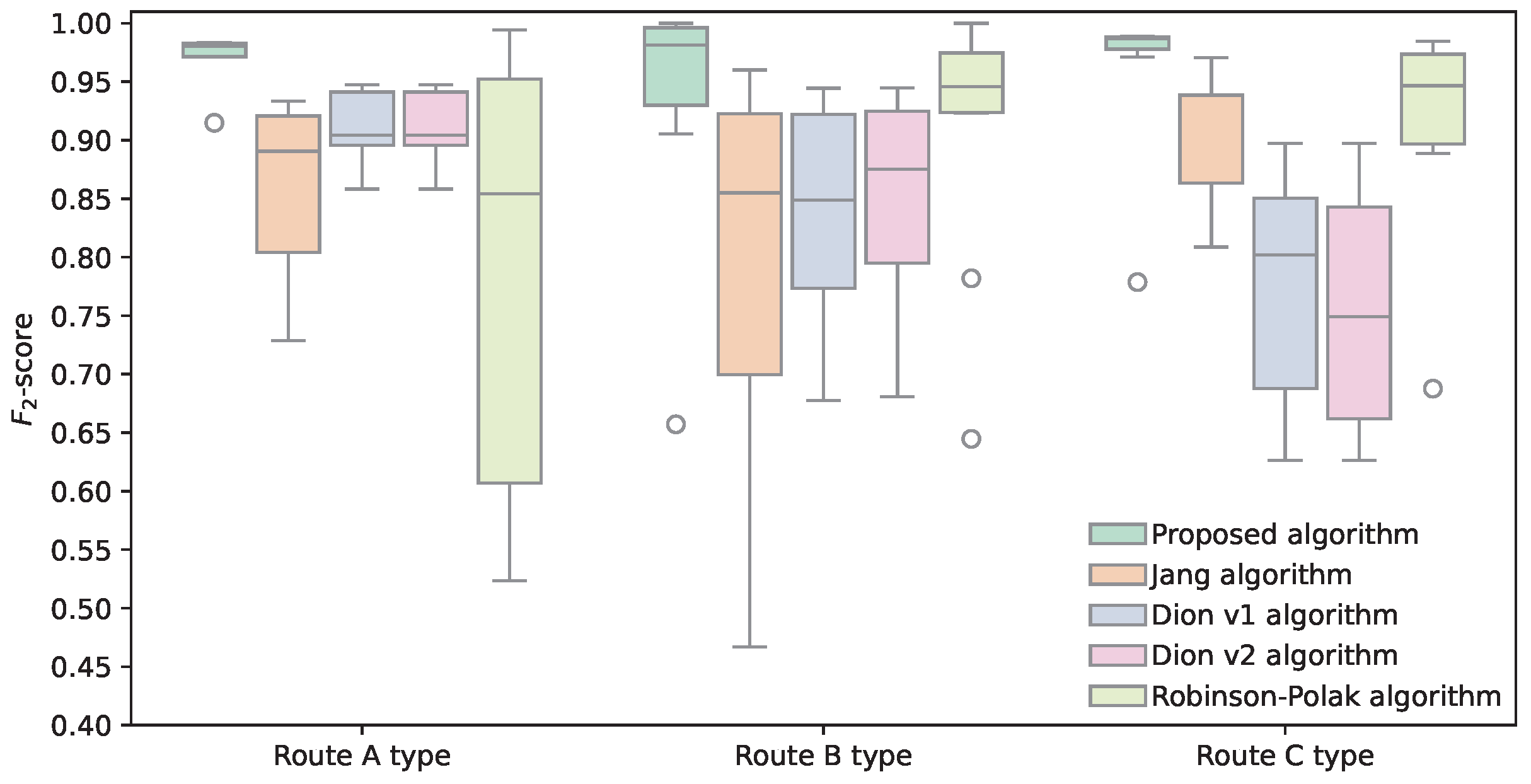
| Route A | Proposed algorithm | 1362 | 3 | 1 | 141 | 0.982 |
| Jang | 1316 | 1 | 47 | 143 | 0.933 | |
| Dion–Rakha v1 | 1353 | 7 | 10 | 137 | 0.947 | |
| Dion–Rakha v2 | 1353 | 7 | 10 | 137 | 0.947 | |
| Robinson–Polak | 1240 | 0 | 123 | 144 | 0.854 | |
| Route B | Proposed algorithm | 2853 | 9 | 1 | 224 | 0.968 |
| Jang | 2595 | 2 | 259 | 231 | 0.812 | |
| Dion–Rakha v1 | 2658 | 42 | 196 | 191 | 0.724 | |
| Dion–Rakha v2 | 2703 | 38 | 151 | 195 | 0.763 | |
| Robinson–Polak | 2757 | 0 | 97 | 233 | 0.923 | |
| Route C | Proposed algorithm | 973 | 5 | 1 | 325 | 0.987 |
| Jang | 945 | 18 | 29 | 312 | 0.939 | |
| Dion–Rakha v1 | 954 | 74 | 20 | 256 | 0.802 | |
| Dion–Rakha v2 | 955 | 113 | 19 | 217 | 0.697 | |
| Robinson–Polak | 809 | 2 | 165 | 328 | 0.905 |
Disclaimer/Publisher’s Note: The statements, opinions and data contained in all publications are solely those of the individual author(s) and contributor(s) and not of MDPI and/or the editor(s). MDPI and/or the editor(s) disclaim responsibility for any injury to people or property resulting from any ideas, methods, instructions or products referred to in the content. |
© 2024 by the authors. Licensee MDPI, Basel, Switzerland. This article is an open access article distributed under the terms and conditions of the Creative Commons Attribution (CC BY) license (https://creativecommons.org/licenses/by/4.0/).
Share and Cite
Richter, P.; Matowicki, M.; Kumpošt, P. Transit Traffic Filtration Algorithm from Cleaned Matched License Plate Data. Appl. Sci. 2024, 14, 8182. https://doi.org/10.3390/app14188182
Richter P, Matowicki M, Kumpošt P. Transit Traffic Filtration Algorithm from Cleaned Matched License Plate Data. Applied Sciences. 2024; 14(18):8182. https://doi.org/10.3390/app14188182
Chicago/Turabian StyleRichter, Petr, Michal Matowicki, and Petr Kumpošt. 2024. "Transit Traffic Filtration Algorithm from Cleaned Matched License Plate Data" Applied Sciences 14, no. 18: 8182. https://doi.org/10.3390/app14188182
APA StyleRichter, P., Matowicki, M., & Kumpošt, P. (2024). Transit Traffic Filtration Algorithm from Cleaned Matched License Plate Data. Applied Sciences, 14(18), 8182. https://doi.org/10.3390/app14188182