2.1. Minimum Enclosing Quadrate Treatment of Leaf Samples
In the classification and recognition of plants, the shape and texture features of leaves are particularly important. However, asymmetric compression operations are often detrimental to maintaining the normativity of these features. As shown in
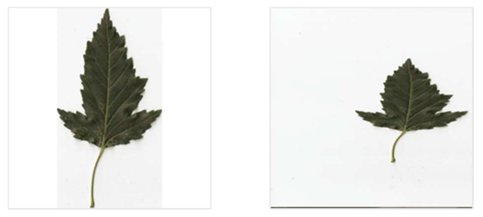
Figure 1, the original sample image is shown on the left, and the compressed image of this sample is shown on the right. In the process of compression, its size is changed from 2544 × 1205 to 224 × 224. It can be clearly seen that the basic characteristics of the leaves have been greatly changed. Obviously, this phenomenon is not conducive to the classification and recognition of the CNN models. It can also be seen that there is a lot of redundant information in the original sample, which will also affect the classification accuracy of the models.
In order to avoid the influence of the abovementioned problems on the classification results, the MEQ method is proposed to standardize the leaf-sample datasets.
Firstly, the RGB image of the leaf sample is converted into a grayscale image by eliminating the hue and saturation information while maintaining the brightness. In this process, RGB values are converted to gray values by calculating the weighted sum of
R,
G, and
B components. The calculation method is given in Equation (1).
where
Gray represents the transformed gray value; and
R,
G, and
B separately represent the red, green, and blue components.
Secondly, the gray image is converted into a binary image to show the leaf contour more clearly. Before that, the Otsu [
18] method is used to calculate the global threshold of the grayscale image. Otsu is an algorithm to determine the threshold of image binarization segmentation, and Otsu is used in this experiment to select the optimal threshold that minimizes the within-class variance of the thresholded black-and-white pixels. The principle of finding the best threshold,
, is as follows.
Let the gray level of a given image be denoted by , and there exists a threshold, , to classify the pixels in the image into 2 classes: class and class . The pixels of class have gray levels of (1, …, ), and the gray level of class pixels is (, …, ).
The within-class variance,
, and between-class variance,
, are expressed as follows:
where
and
are the probabilities of occurrence of class
and
, respectively;
denotes the variance of class
; and
denotes the variance of class
. In addition,
and
, respectively, represent the average gray values of the two categories, and
represents the total average level of the grayscale image.
Since
is always true (where
is the total variance), the sum of the within-class variance and the between-class variance is fixed, which means that the maximum between-class variance is the minimum within-class variance. So, the optimal threshold,
, should satisfy the following equation:
And the search for the maximum,
, can be restricted to the following:
Here,
and
where
and
are the zeroth- and the first-order cumulative moments of the histogram up to the
th level, respectively. And
denotes the probability that a pixel with gray value
appears in the image.
Therefore, according to the obtained optimal threshold, , all values greater than the threshold in the grayscale image are replaced with 1 (white), and all other values are set to 0 (black) to obtain the binary image of the sample.
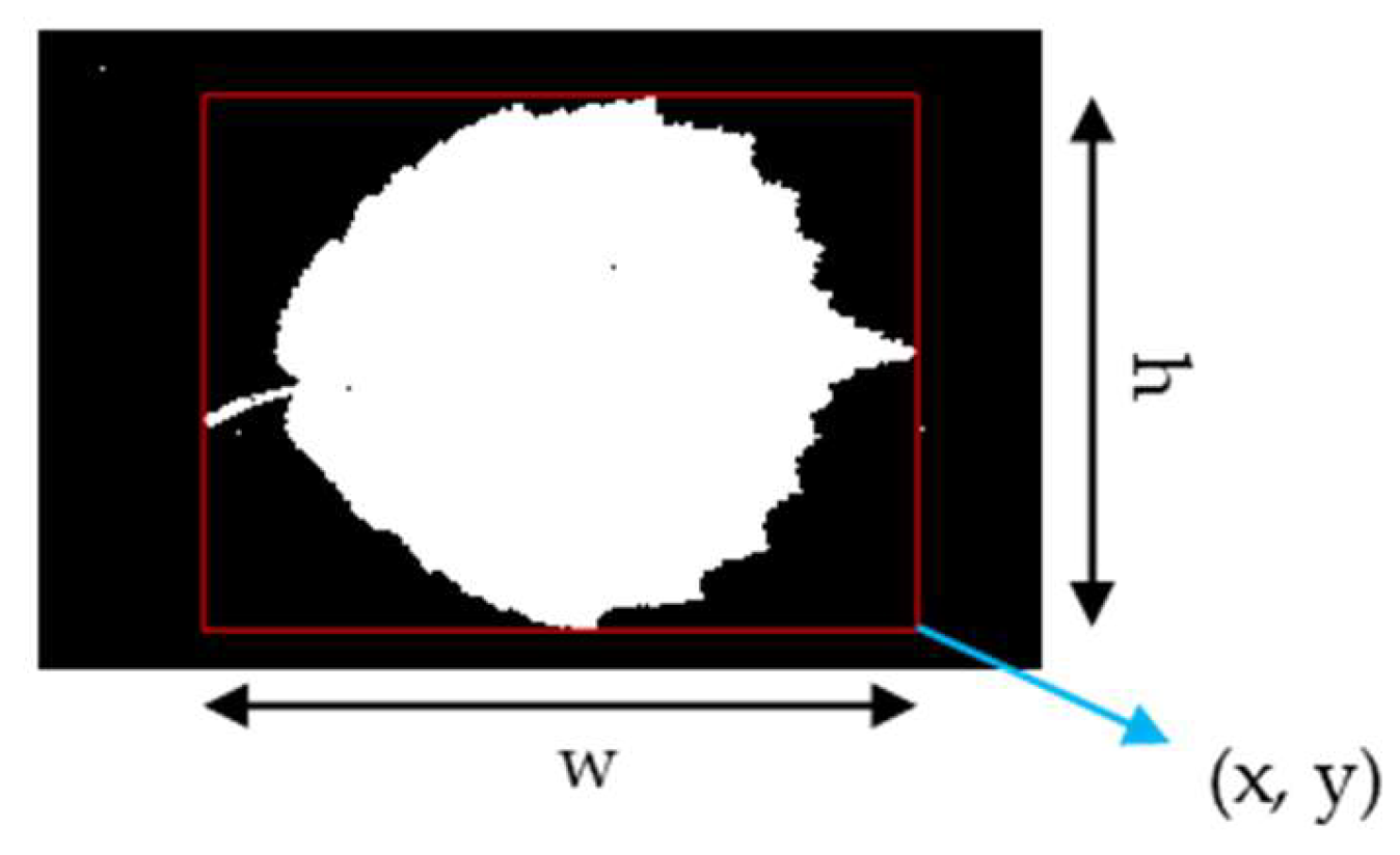
After that, the next work is to find the minimum enclosing quadrate of the sample. To do this, we need to find the minimum enclosing rectangle (MER) of the sample. MER refers to the maximum extent of some 2D shape (e.g., points, lines, and polygons) represented in 2D coordinates, that is, a rectangle bounded by the maximum abscissa, minimum abscissa, maximum ordinate, and minimum ordinate of each vertex of a given 2D shape. However, due to the interference of the image background and redundant information, directly calculating the MER of sample binary images cannot achieve the desired effect. Consequently, in this paper, the method of finding the maximum connected component of the image is adopted to obtain the MER of the leaf. We take the area of each object (connected component) in the image and create a rectangle parallel to the axis in 2D coordinates. As shown in
Figure 2,
is defined as a rectangular four-element vector (expressed in data units). The point
represents the lower-right corner of the rectangle and is used to determine its position. The
and
denote the length and width of the rectangle, respectively, and are used to determine the dimensions of the rectangle. Then, the four-element vector of the rectangle with the largest area in the image is recorded, which is the MER of the leaf. The search for the rectangle,
, can be determined according to the following expression:
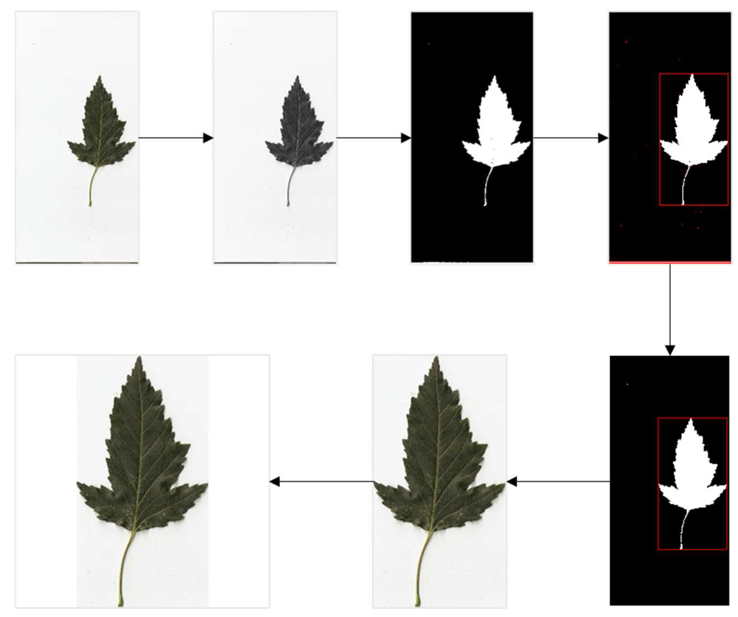
Finally, according to the recorded coordinate data, the target area is cropped out in the original color sample image. The shorter side of the rectangle is symmetrically extended on both sides, transforming it into a square. It should be mentioned that, considering the importance of leaf edge information, we retain part of the background information of leaf edges.
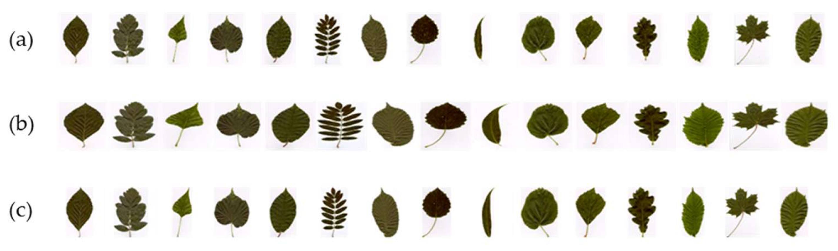
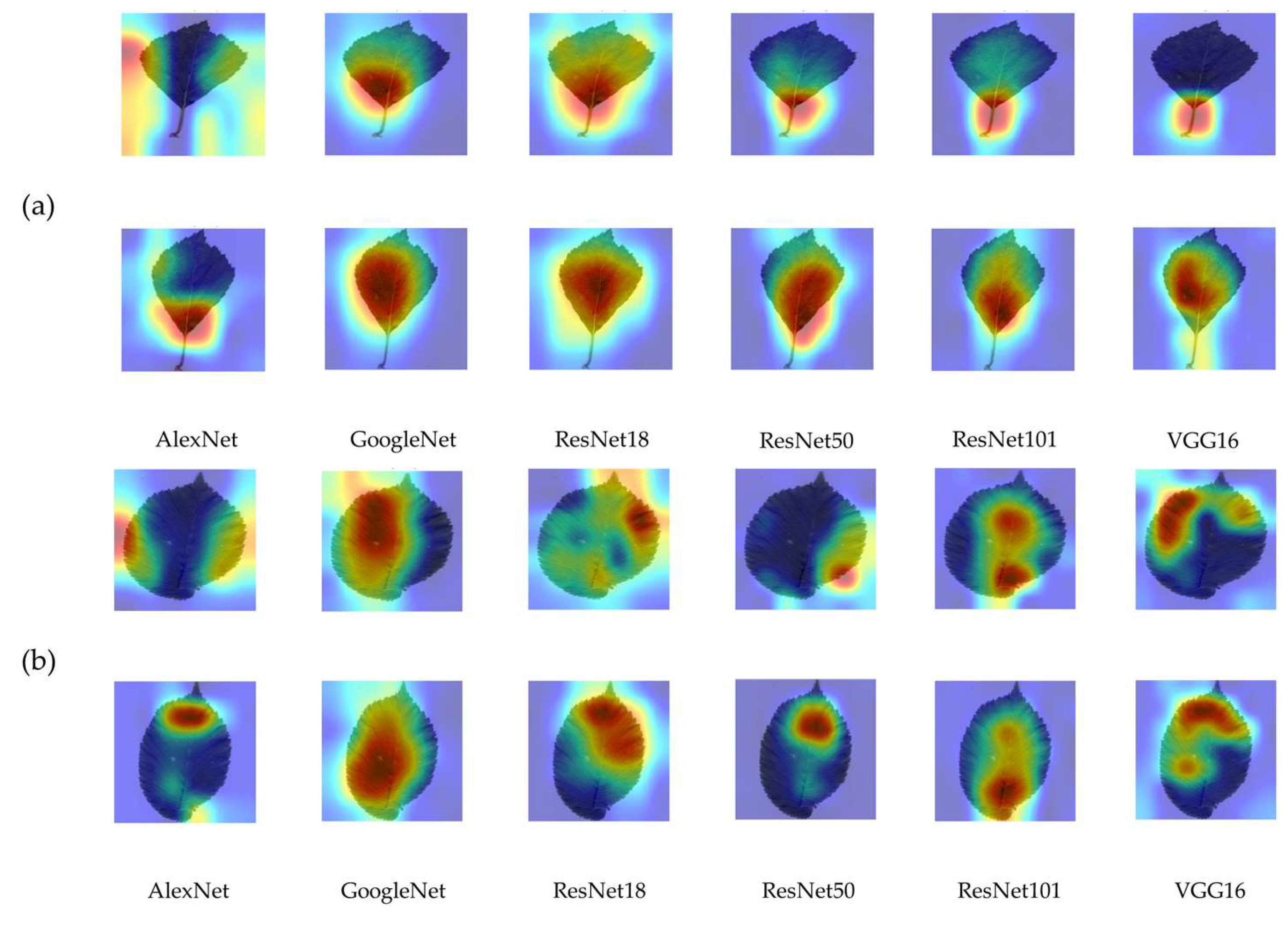
Figure 3 shows the standardization process of a sample, and
Figure 4 shows the compressed images of the standardized sample and the original sample, which is from the MEW2012 leaf dataset. From
Figure 3, it can be found that the sample processed by the MEQ method not only fully retains the main characteristics of the leaf but also eliminates most of the redundant information in the image. It can also be clearly seen from
Figure 4 that the characteristics of the original sample have changed greatly after direct compression. Different from them, the MEQ method ensures the standardization of the sample features, and the texture information of the leaf also becomes clearer, which is very helpful for the feature extraction of the CNN models.


