3.1. Factors Influencing the Performance of Thrust
In this section, the effects of , , and on push force are analyzed based on the experimental results. The parameters that make the push force output more stable are selected and used to verify the accuracy of the measurement method in this paper.
We set the weight of the bit to 1 MPa and the rotational speed
= 120 rpm to test the push force output under different inclination angles. Because of the unsatisfactory reduced deviation control effect of the N-MVDT when
is low (
), and because the main focus of this paper is on the degree of performance improvement in the MVDT by the TID, the range of
in this experiment was limited to 1~5°. In the tool inclination correlation analysis
, the average value of the output pushing force of each hand was used. The experimental result is shown in
Figure 15.
According to
Figure 15, when
is small (
≤ 1), the difference between
in the respective prototypes is similar. However, when
is larger (
≥ 3), the
values of the USR are similar and significantly larger than the
values of LSR in the respective prototypes. This indicates that the O-MVDT and the N-MVDT effectively reduce the inclination of the wellbore when
is large. Therefore, the reliability of the corrective function of the O-MVDT and the N-MVDT was preliminarily confirmed.
Furthermore, for = 2, there is no notable disparity in the value of the O-MVDT, whereas the value of the LSR in the N-MVDT is marginally lower than the corresponding value of the USR. This suggests that the N-MVDT has a superior capability to reduce the wellbore inclination than the O-MVDT at = 2.
It should be noted that other MVDT structures can still maintain their normal inclination deviation correction function even at very low values of . However, for the N-MVDT, the inclination deviation function is gradually lost when . Since this paper focuses on studying the improvement effect of the TID on the N-MVDT, experimental data with > 2 were selected to compare the inclination deviation effects between the O-MVDT and the N-MVDT in subsequent studies.
Additionally, the
values observed in the O-MVDT are marginally higher than their counterparts in the N-MVDT for all
values. This discrepancy could potentially stem from the N-MVDT’s intricate design, which encompasses multiple elements like the adjusting device. These components contribute to a heightened pressure drop in the drilling fluid, as stated in [
31], subsequently resulting in a decreased inlet pressure within the N-MVDT’s channel.
The speed was set to 120 rpm and the inclination was 3°. The push force under three different sets of bit weights was obtained through the experiment based on the principles of the executing agency described in
Section 2. After increasing the weight on the bit, since the magnitude of
is dependent on the pressure difference between the inside and outside of the drilling tool [
32], a larger
results in a larger
. According to the data in
Figure 16, the
of the N-MVDT is slightly lower than that of the O-MVDT. Since the difference between the high and low edge
values is more obvious at a higher bit weight,
P = 1.5 MPa was selected as the experimental parameter for use in the subsequent experiment.
When comparing the push force alterations at the well’s upper and lower sides, analyzing the variations in the upper side proves to be more straightforward.
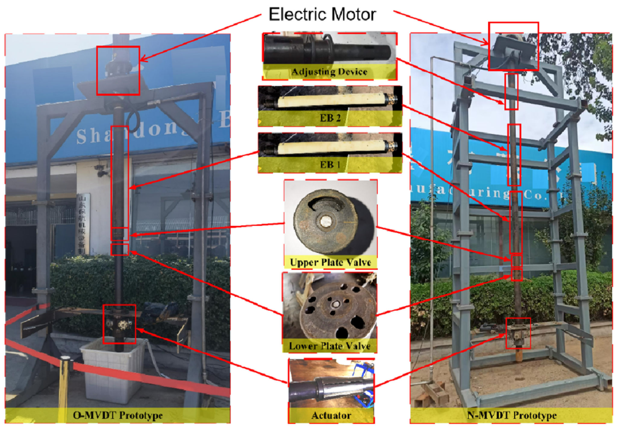
Figure 17 illustrates the output curve of the tested drill tool’s high-side hand push force at varying speeds. Notably, the O-MVDT’s force sensor, denoted as
, underwent two and three complete cycles at rotational speeds of 90 and 120, respectively, indicating a direct correlation between the number of cycles and the increase in speed. However, at slower rotational speeds, EB 1 encountered static friction from the upper plate valve, causing it to rotate in unison with the shell, which poses a potential issue. Consequently, to streamline the subsequent analyses, a rotational speed of
= 120 was chosen as the preferred option.
The above regularities are consistent with the experimental data, indicating that the fundamental design objectives were achieved for both prototypes and confirming the reliability of the experimental data. To visually compare the stability differences between the O-MVDT and the N-MVDT, the operating conditions of = 3, = 120, and = 1.5 were selected for the experimental parameter.
3.2. The Difference in Performance of the O-MVDT and the N-MVDT
According to the experimental parameters selected in
Section 3.1, the push-back performance of the two kinds of vertical drills was tested, and the output curves of the force of the two kinds of vertical drill was obtained under the selection of
= 3,
= 120, and
= 1.5.
Figure 18(a1,a2) show
in the O-MVDT and the N-MVDT, respectively. The graphs reveal that the
values of the LSR are similar and lower than the
values of the USR in both prototypes, and the data fluctuations are regular. This indicates that both prototypes were in a relatively stable condition during the measurement.
It should be noted that when the drilling tools were tilted, the upper arc hole should have remained stable at the upper side of the well bore. While there should be no drilling fluid passing through the channel of the LSR, the
values of the LSR in both prototypes were not zero, as depicted in
Figure 18(a1,a2). This is due to the small gap between the two plate valves, which allows for the drilling fluid to enter the channel of the LSR [
33], leading to non-zero
readings.
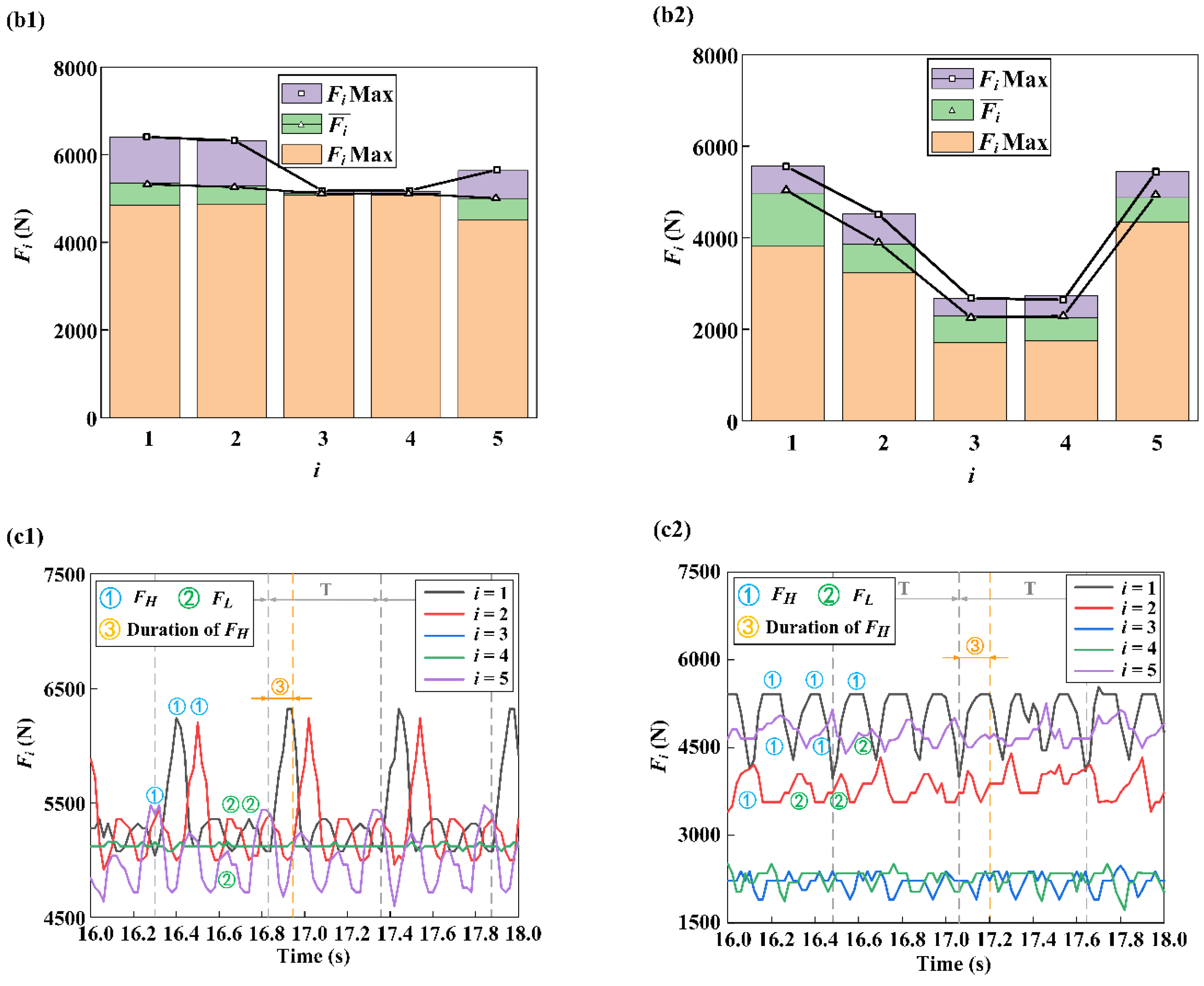
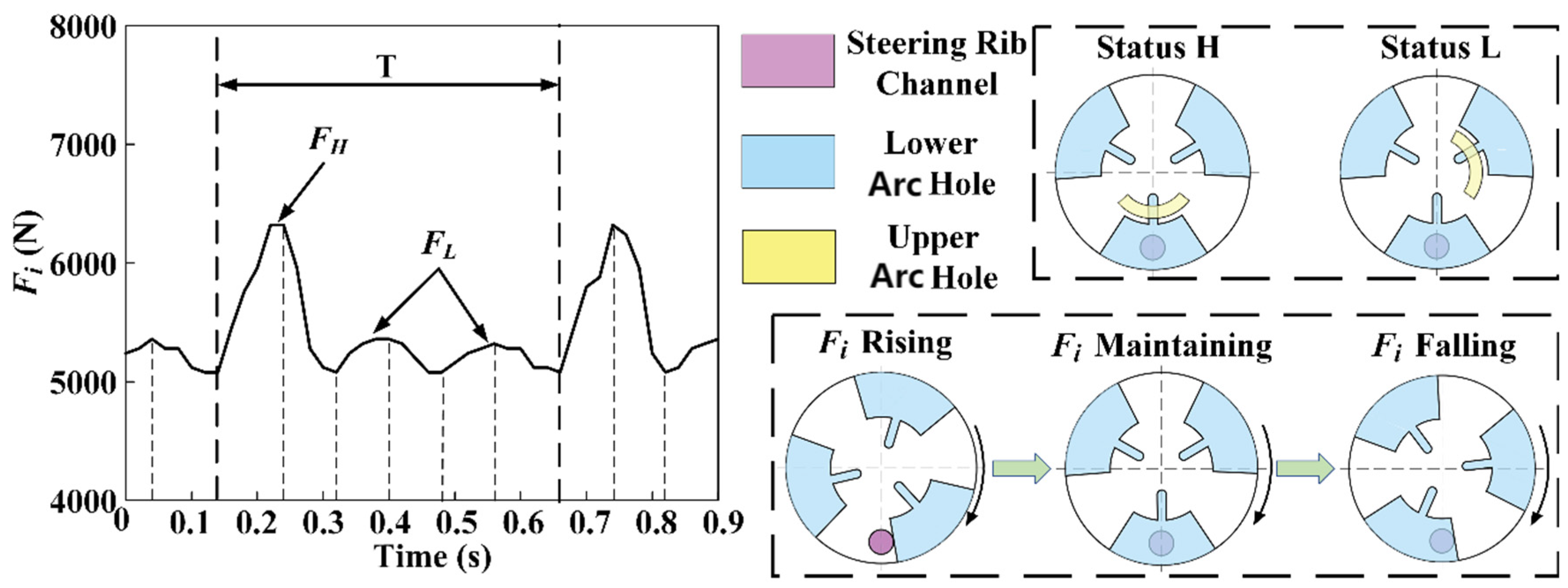
The three waves of
may exhibit different patterns in a single period, as depicted in
Figure 18(c1,c2). When a “rising–falling” or “rising–stable–falling” wave is more prominent within a period, it is referred to as a higher pushing force (
), while considerably smaller waves are referred to as a lower pushing force (
). The distinction between
and
is evident in
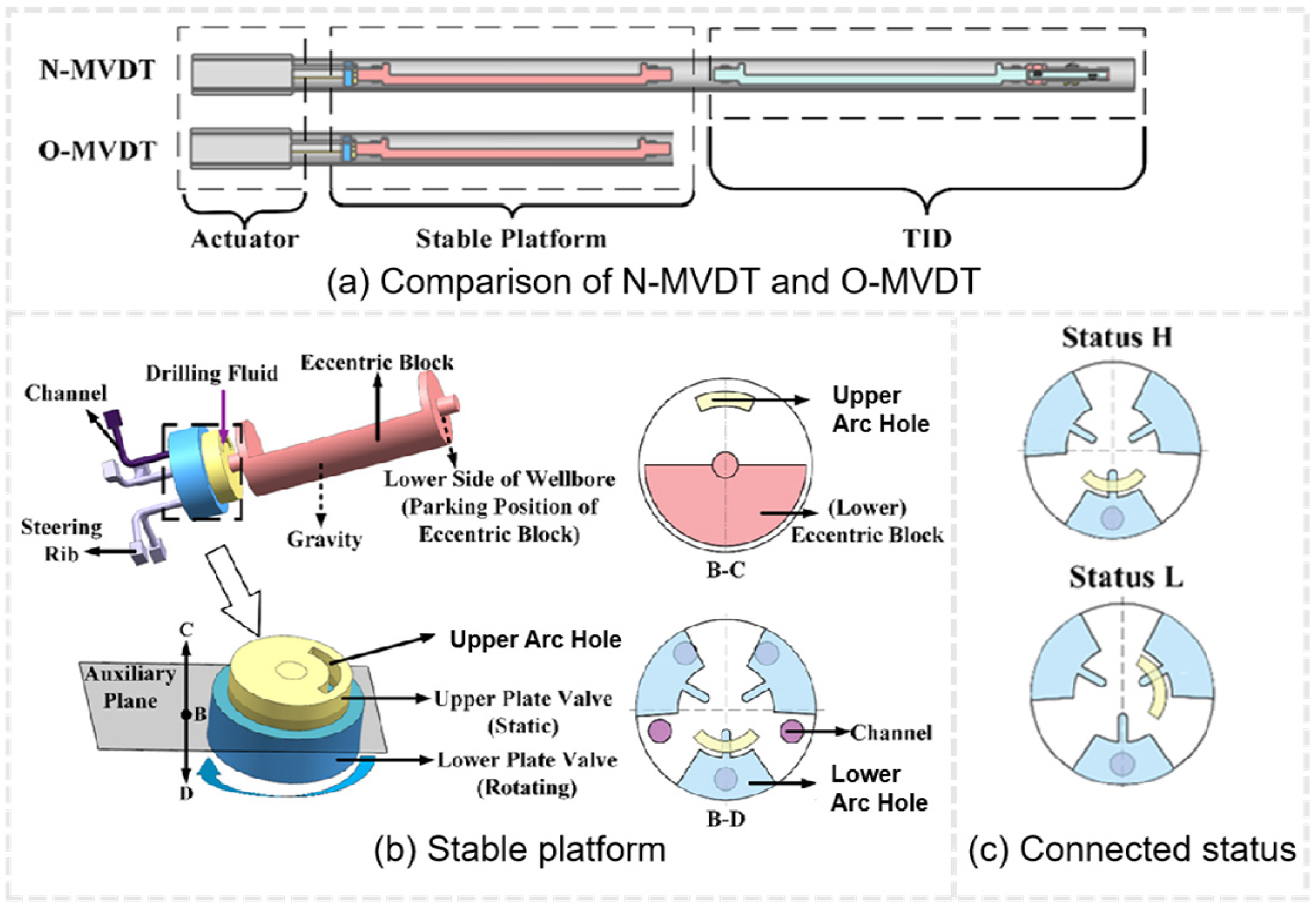
Figure 18(c1,c2). When a channel, an upper arc hole, and one of the lower arc holes are all connected, this connection status is referred to as status
H. During status
H,
starts to rise as the drilling fluid flows into the channel, and it remains high for the duration of this status.
falls when the connection is not in status
H.
occurs during status L when the drilling fluid flows into the channel through the gap between the upper and lower plate valves, even when the upper arc hole is not connected. At this moment,
will slightly increase, resulting in the appearance of
. Moreover, it is expected that the upper plate valve and EB 1 will be stabilized in their final positions. In this scenario, if
occurs, there should be three identical
in one period. However, in reality,
and
exist simultaneously in one period, indicating that EB 1 is not completely static.
The analysis above indicates that the function of EB 1 for detecting well inclination remains effective even in a partially static condition. For simplicity, we define State 1 as when EB 1 or upper plate valve is completely static, State 2 as when EB 1 is not completely static but does not affect the inclination correction of the drilling tool, and State 3 as when EB 1 is completely unstable.
In State 1, will display three identical waves during each period. In State 2, the upper plate valve will not be stationary and will oscillate within a small range because of the slight rotation. Consequently, both status L and status H will occur simultaneously during one period for a given channel, resulting in the presence of both and .
The above law applies to both the O-MVDT and the N-MVDT, but there are significant differences between the two prototypes in terms of
. The magnitude of
differs between the prototypes, as shown in
Figure 18(a1,a2). In the O-MVDT, the sequence of
is
, whereas in the N-MVDT, the sequence of
is
. This indicates that the position of the upper arc hole is different in the two prototypes because of the influence of the adjusting device. The different positions of the upper arc hole result in different flows of the channels and change the magnitude sequences of
.
The statistics of
are presented in
Figure 18(b1,b2), which shows that in the N-MVDT, the average and maximum values of
for the USR are significantly larger than those for the LSR. In contrast, the differences among these values are relatively small in the O-MVDT. This suggests that EB 1 is more stable under the action of the adjusting device in the N-MVDT, and the lower arc hole stays longer at the USR compared with the O-MVDT.
Furthermore, the duration and frequency of in the USR of the N-MVDT are longer and higher, respectively, compared with the O-MVDT. Specifically, of in the N-MVDT appears three times in one period and occupies almost the entire period, while in the O-MVDT, there is only one of in one period with much less duration.
As the lower arc hole rotates at a uniform speed and passes through one channel three times in one period, in State 2, the duration of status H is longer than the duration of status L when the upper arc hole stays in the position of this channel for a longer time. As the lower arc hole rotates at a constant speed, it traverses a channel three times within a single cycle. In State 2, the duration of status H surpasses that of status L because of the upper arc hole’s extended presence within the channel’s position. As a result, more appears, and the duration of is longer. By combining the data on all , it can be concluded that the upper arc hole stays longer at the USR, and the value of comes closer to the theoretical lower side in the N-MVDT than in the O-MVDT.
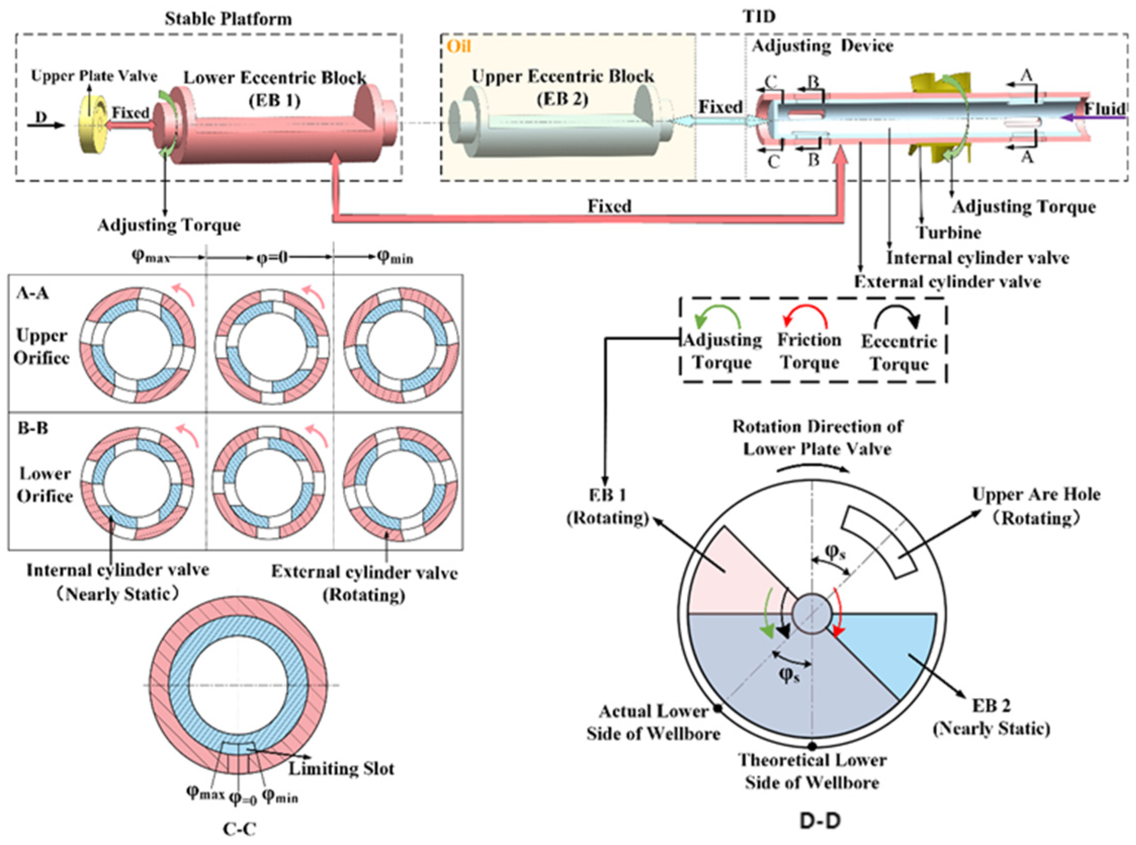
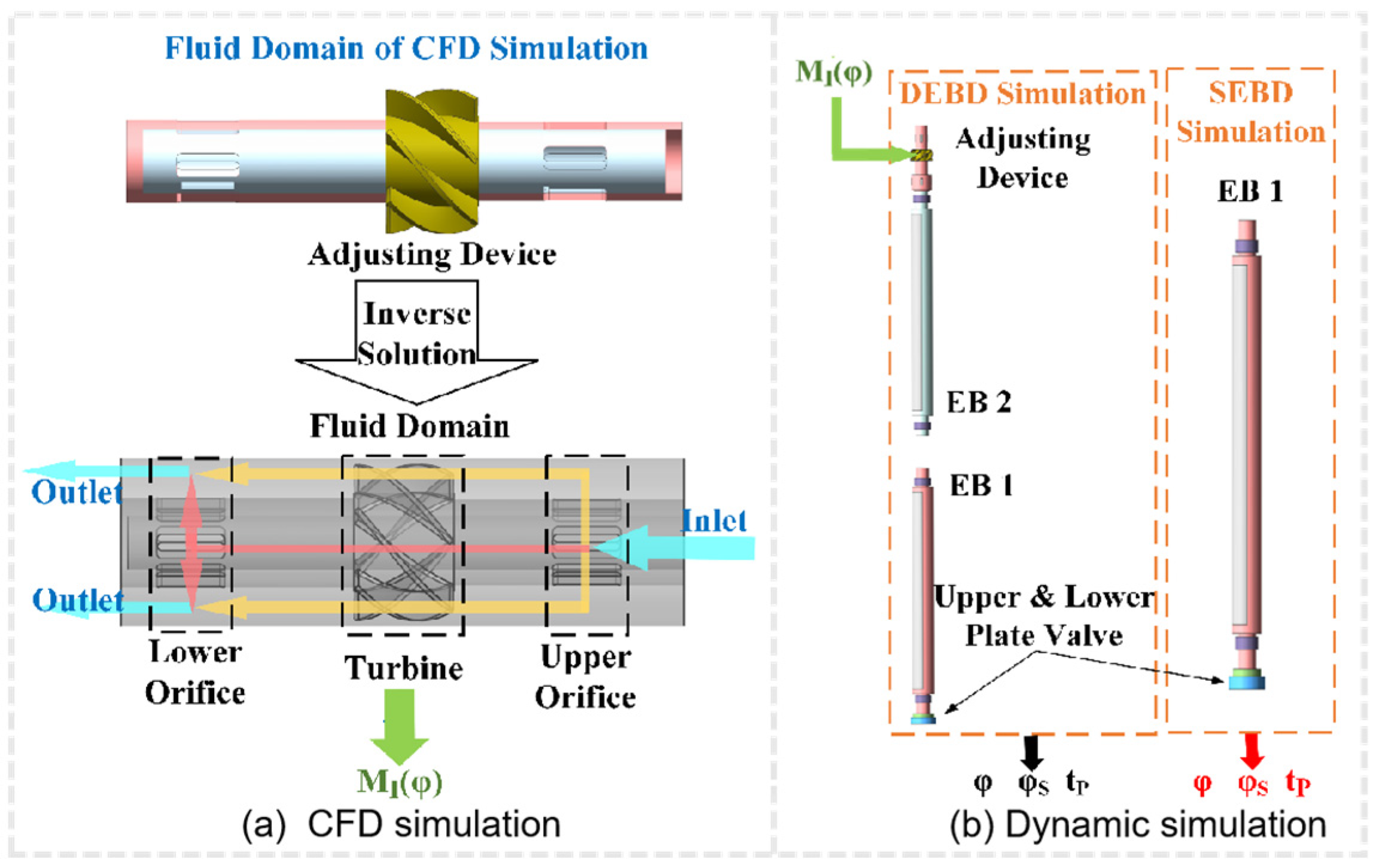
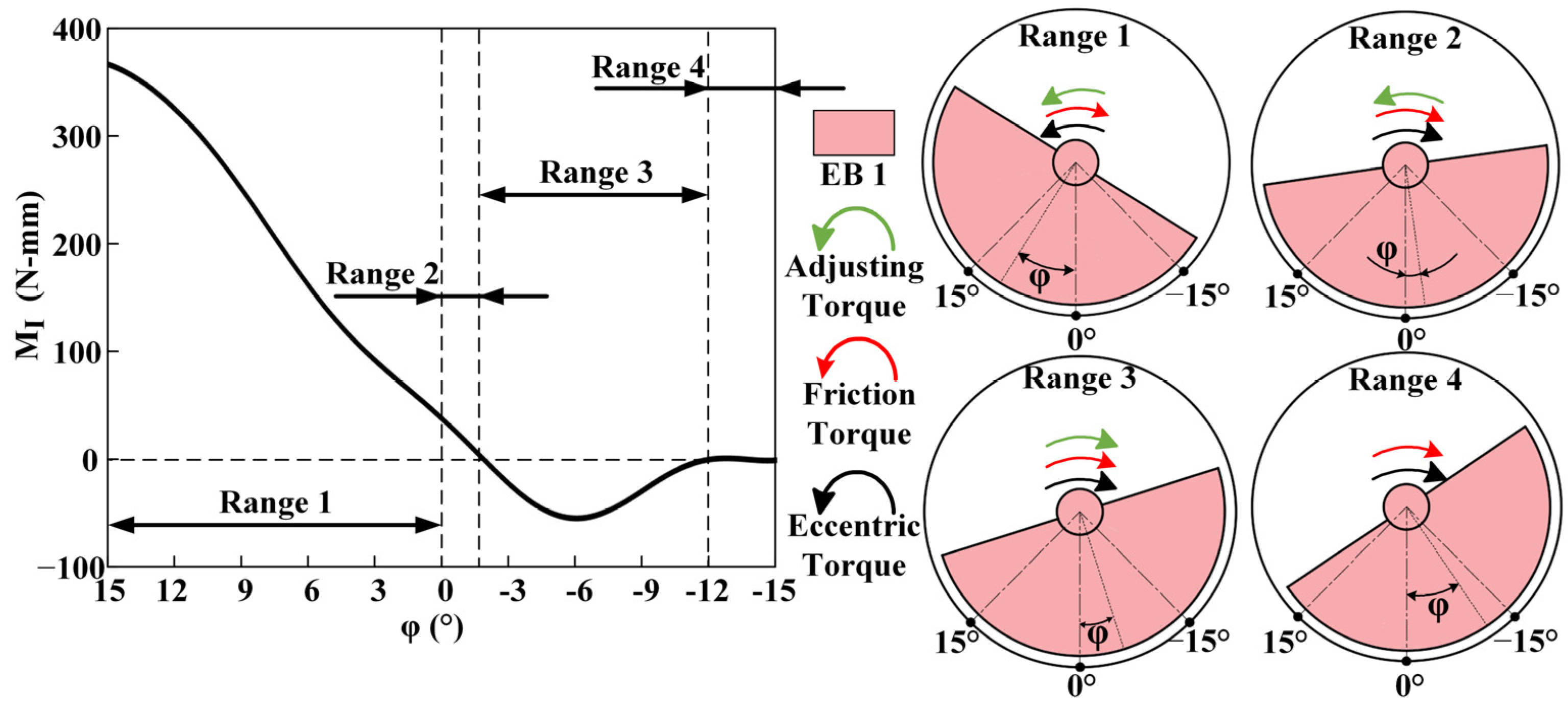
The adjusting device of the TID operates in a fluid environment within the downhole. The adjusting torque, denoted as , can be obtained through computational fluid dynamics simulation (CFD simulation).
First, the three-dimensional fluid domain model of the adjusting device and rotation of the fluid domain of the external cylinder valve were derived to represent its rotation under the influence of EB 1. When the value of
is different, the fluid domain of the orifices in the external cylinder valve will rotate to different angles, resulting in different fluid flow rates passing through the turbine. The turbine at different values of
is obtained through CFD simulation (as shown in
Figure 19), which considers the flow area of the upper and lower orifices, as illustrated in
Figure 3. As EB 1 deflects in the direction of the balanced friction torque, the positive direction of
is defined as such. Equivalently, the positive orientation of
is designated as being opposite to the frictional torque experienced by the upper plate valve.
When is in range 2, the flow area of the upper orifice is smaller than that of the lower orifice, but remains positive. Despite its opposite direction to the friction torque, moves away from zero and reduce negatively at this point.
When is in range 3, the smaller flow area of the upper orifice and the negative produce a combined effect that brings closer to zero, despite the direction of being the same as the friction torque.
When is in range 4, the upper orifice is nearly closed, and the lower orifice is almost completely opened. is approximately zero, and approaches zero under the combined effect of the two torques, without any adjusting torque.
Although briefly becomes negative because of reflux, its magnitude is small, and it helps to bring from negative values closer to zero as the eccentric block swings because of inertia. Furthermore, since the direction of the friction torque is constant, is generally not negative. Therefore, by outputting the adjusting torque, the adjusting device can be closed-loop to bring closer to zero.
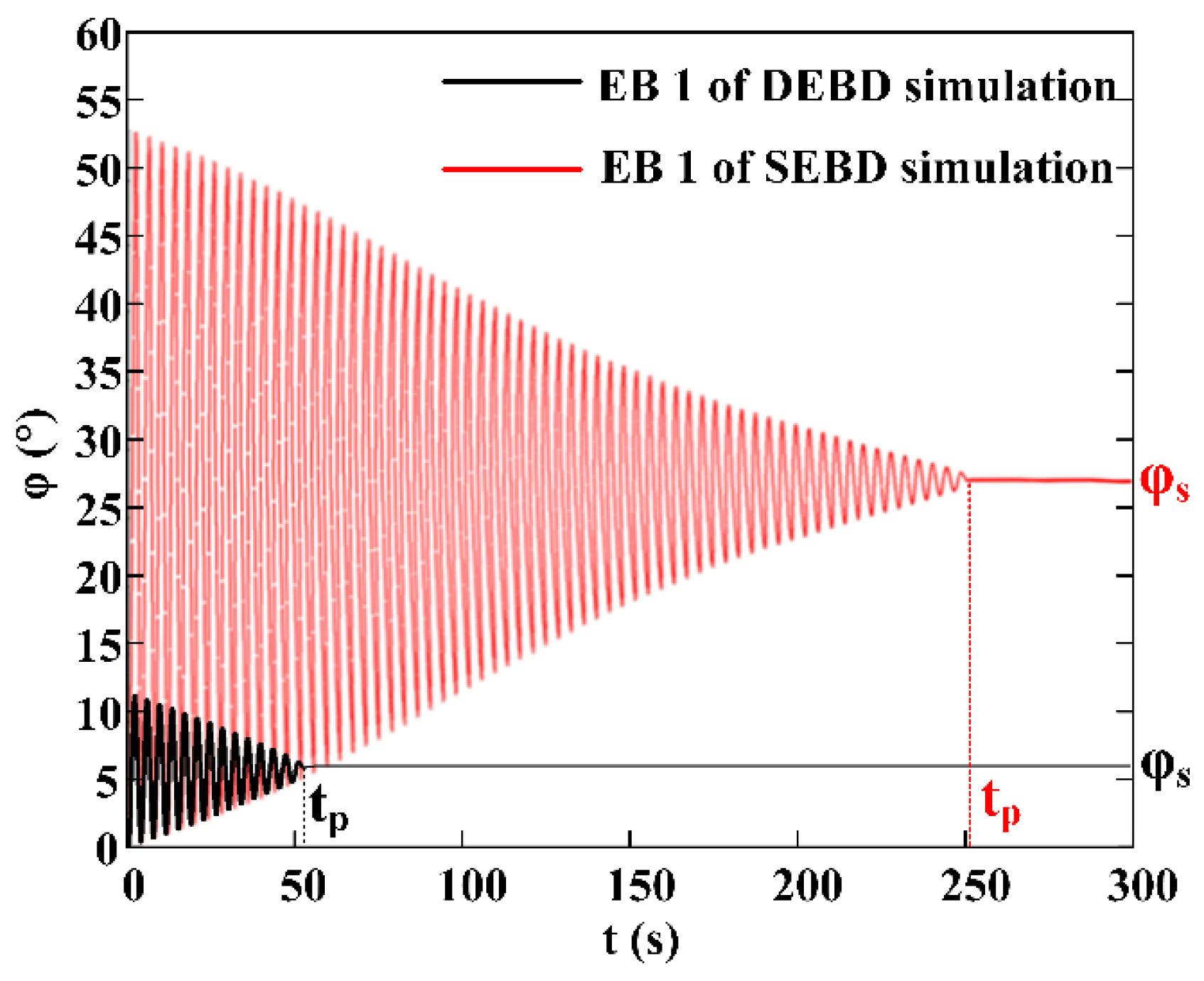
For a stable platform,
changes instantaneously with time under the action of multiple moments in EB 1, and EB 1 stabilizes at
after the stable time (
). These three parameters (
,
, and the range of
) can be obtained by multibody dynamics simulation [
34] and can be used to evaluate the results of the simulation. The stability of EB 1 is better when
is shorter and the range of
is smaller. The stability is also reflected when
is closer to zero.
The curve of the fail over time in the DEBD simulation and the SEBD simulation was obtained after inputting the adjusting torque, as illustrated in
Figure 20.
The main difference between the DEBD simulation and the SEBD simulation is that is shorter in the DEBD simulation. Additionally, the range of in the DEBD simulation is much smaller, approximately [0°, 11°], compared with the SEBD simulation, which has a range of approximately [0°, 55°]. Finally, is approximately 5° and 27° in the DEBD simulation and SEBD simulation, respectively.
In summary, increasing the adjusting torque of EB 1 significantly reduces , , and the range of . The simulation results demonstrate that the TID can achieve its design purpose, and increasing the TID will improve the stability and reduce the deviation control accuracy of the N-MVDT. The experimental results in this paper confirm that because the pressure loss caused by the regulating device, the pushing force of the improved N-MNDT decreases compared with that of O-MVDT. However, because the time of the development of the TID is short, there are still some drawbacks. Therefore, the current N-MVDT is suitable for drilling conditions with small pushing force and high accuracy requirements. The flow channel structure can be optimized and improved to solve this problem.
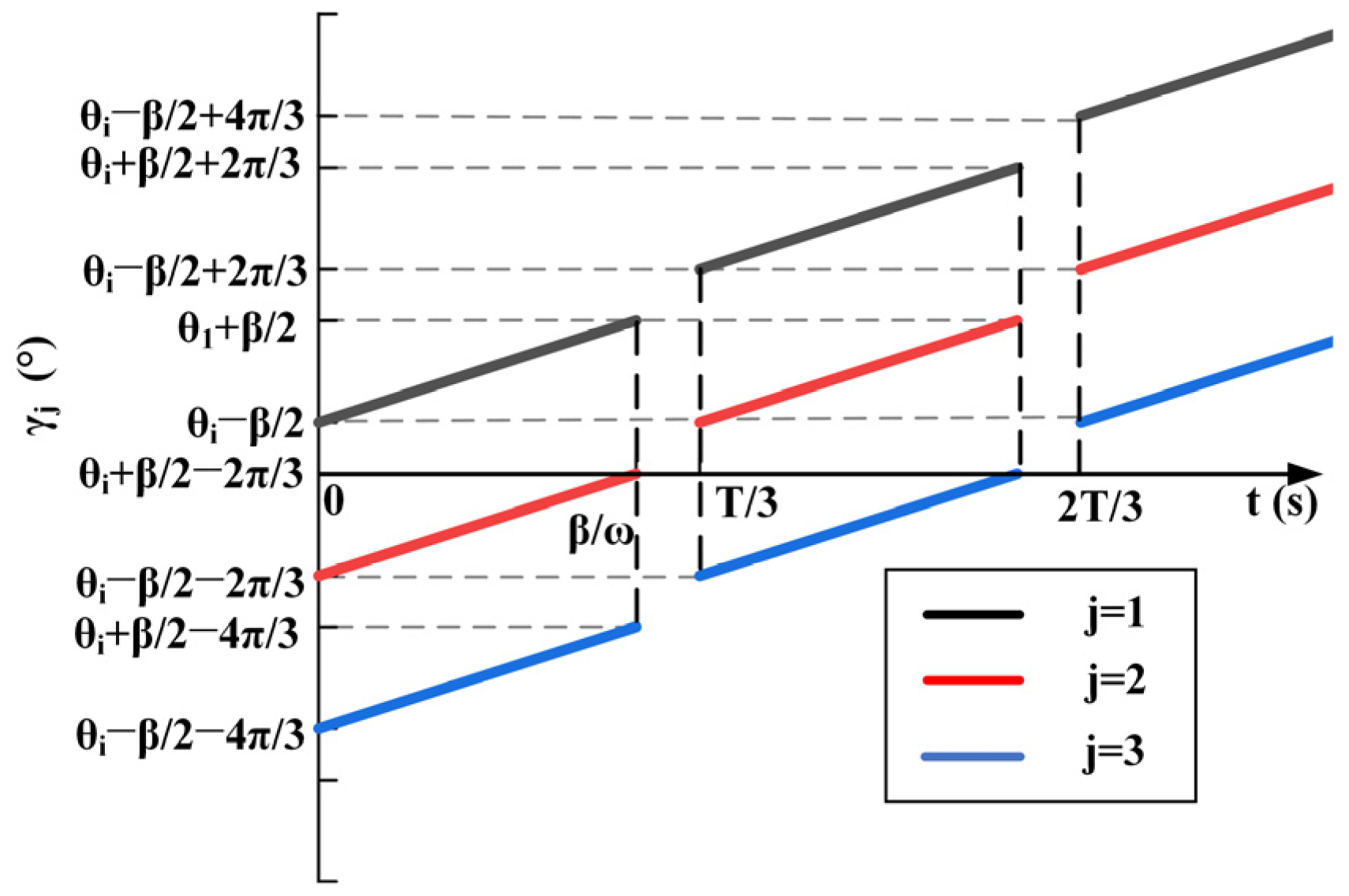
3.3. Measurement Accuracy Analysis
According to the results of the experiment, the fluctuations in
showed a regular periodic pattern, as illustrated in
Figure 18(c1,c2). Each period of
contained three waves. This can be attributed to the design of the lower plate valve, which has three arc holes that align with the channel as the valve rotates. This creates three instances of what is referred to as status L within one period of rotation. During status L,
starts to rise and remains elevated until the valve moves out of the status L position, at which point
begins to fall again, as shown in
Figure 21.
Figure 21.
Diagrams and reasons for the appearance of
and
.
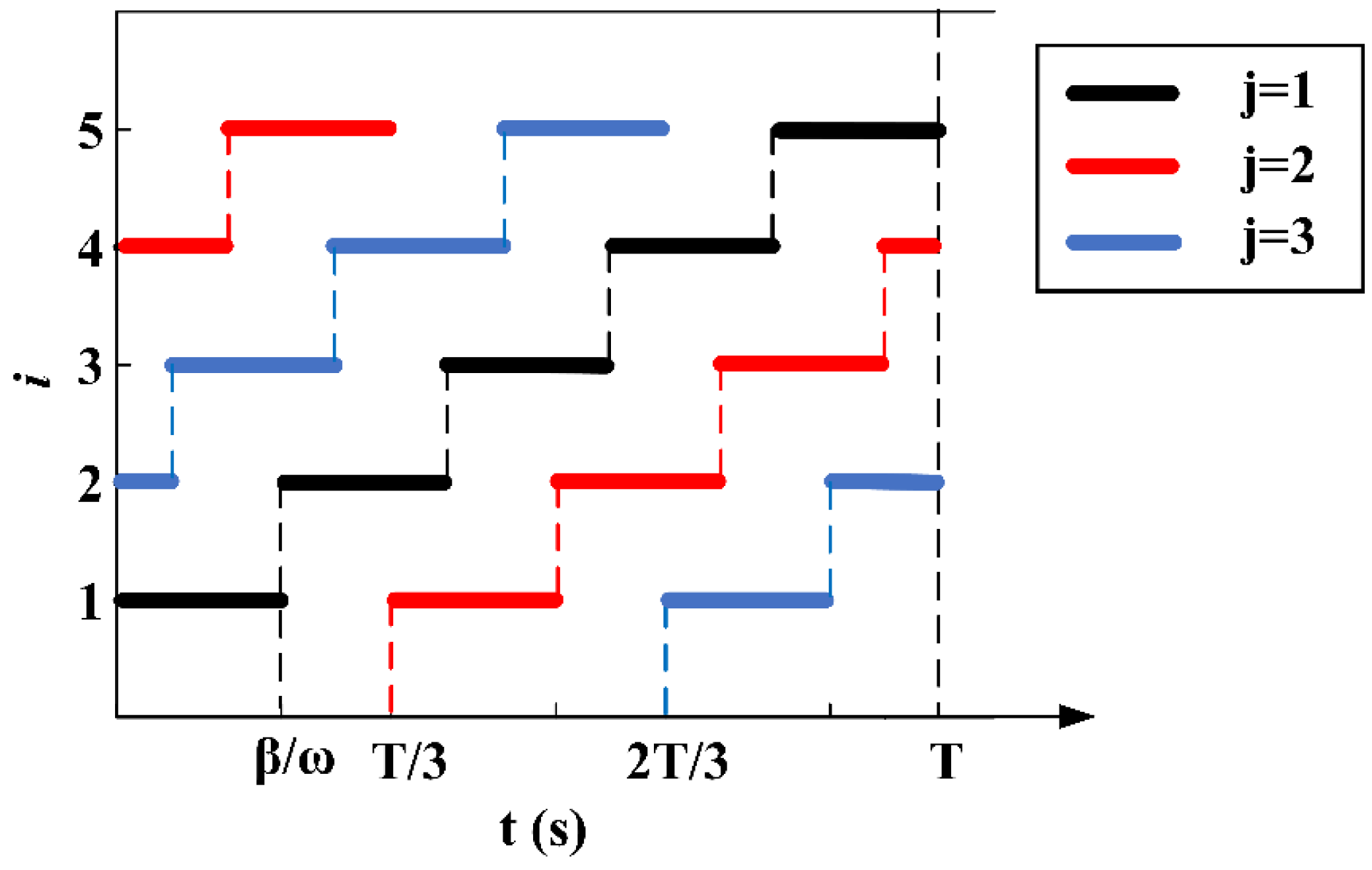
Table 6 shows all the
numbers of
in one period.
Figure 21.
Diagrams and reasons for the appearance of
and
.
Table 6 shows all the
numbers of
in one period.
Table 6.
Comparison of numbers in one period of the O-MVDT and the N-MVDT under .
Table 6.
Comparison of numbers in one period of the O-MVDT and the N-MVDT under .
|
| Numbers of the O-MVDT | Numbers of the N-MVDT |
|---|
| 1 | 1 | 3 |
| 2 | 1 | 1 |
| 3 | 0 | 0 |
| 4 | 0 | 0 |
| 5 | 2 | 2 |
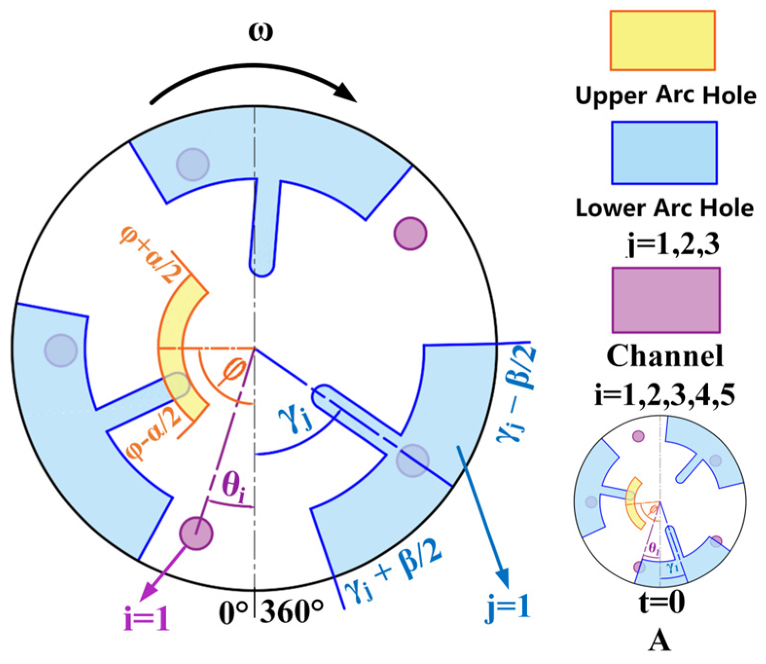
Specifically, to simplify the calculation, if there are three
in one period of
, and each
has a longer duration (almost one-third of the period, as shown by
in
Figure 18(c2)), it can be assumed that the steering rib
is in the through flow state (or status H) at any time. At this moment, Equation (11) can be simplified as:
If there is no
in one period of
, the steering rib
i cannot flow through via the upper arc hole at any time. In this case, (12) can be simplified as:
The range of can be solved according to using (9)–(12), (16) and (17).
In conclusion, the experiments and analysis of the O-MVDT and N-MVDT prototypes revealed significant changes in the rotating situation of the upper plate valve. The adjusting torque on EB 1 balanced the friction moment and reduced the value of . In the N-MVDT, the range of was smaller and was closer to the theoretical lower side. Additionally, in State 2, the N-MVDT had more numbers and a longer duration of . Despite reducing the magnitude of , the addition of the TID improved the stability of the upper plate valve and . These findings demonstrated the successful operation of the TID.
The deviation angle range of the O-MVDT and the N-MVDT obtained from mathematical models was used to obtain the mathematical model of the instantaneous deflection angle and analyze the optimization effect of the TID on the N-MVDT’s stability. In this section, we calculated the range of based on the experimental data.
Because of the large amount of data, only a portion was selected for analysis. The selected data had the same parameters as in
Section 3.1 as follows:
= 5,
= 120, and
= 1.5. The parameters in the model for this operating condition are shown in
Table 7.
The wave situation of
in one period for the O-MVDT and the N-MVDT is shown in
Table 6. For
of the N-MVDT, we can obtain the range of
through (16):
For
of the N-MVDT, the range of
can be obtained using Equation (17).
Through Equation (10), we can calculate the range of
for
of the N-MVDT:
The range of
for
and
of the N-MVDT can be obtained using Equation (17):
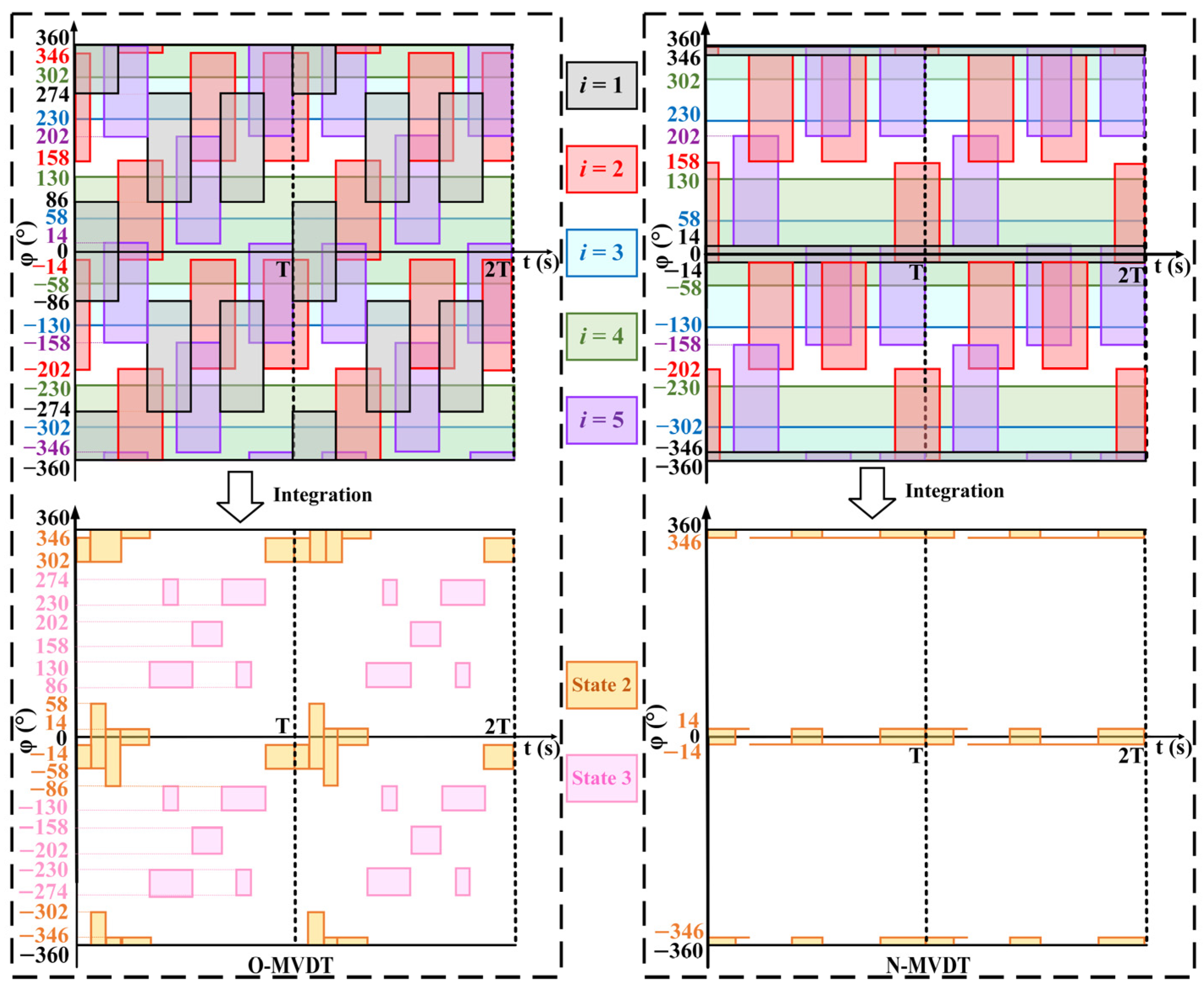
Using (18) to (22), we can calculate the range of
with respect to
in the N-MVDT. We can apply the same method to obtain the range of
with respect to
for the O-MVDT, as illustrated in
Figure 22.
The range of is more clearly defined when the upper plate valve is in State 2. When it is in State 3, although can still cause flow in the corresponding channel, the movement of the upper plate valve is irregular, and the range of is less accurate. However, the upper plate valve will eventually return to State 2 after some time.
During the N-MVDT’s operation, the upper plate valve remains in State 2 for almost the entire time, allowing for a controlled range of within [−14°, 14°]. On the other hand, during the O-MVDT’s operation, the range of is much larger at [−86°, 58°] when the upper plate valve is in State 2, and the duration of State 2 is much shorter compared with the N-MVDT. The TID effectively decreased the range of and increased duration in State 2, indicating that the MVDT’s stability was improved. Moreover, the range of was more uniformly distributed in the N-MVDT, providing further evidence that the N-MVDT’s stability is superior to the stability of the O-MVDT, which demonstrates the effectiveness of the TID in achieving the desired design objectives.
In this section, the experimental data was fed into the derived relationship, and the specific angle range of phi was obtained. The accuracy of the mathematical model was validated by the comparison of simulation and experimental results.
Additionally,
Table 8 presents a comparison between the range of
obtained from the model and simulation. The main source of error comes from the negative range of
, which is caused by the inertia of EB 1 during the experiment, leading to rotation in the negative direction of
. However, the error in the positive range of
is small, indicating the reliability of the model.


