A Novel Algorithm for Optimal Discretization of Stress–Strain Material Curves for Application in Finite Element Analyses

Featured Application

The maximal vertical distance (MVD) algorithm is intended to be used for the discretization of stress–strain metallic material curves for defining a multilinear material model when conducting a finite element analysis of engineering components with included material nonlinearities.

Abstract

The maximal vertical distance (MVD) recursive algorithm, a novel approach for the optimal discretization of stress–strain material curves, is proposed. The algorithm simplifies the process of defining multilinear curves from material stress–strain curves when conducting a finite element analysis (FEA) of components. By directly selecting points on the material curve, the MVD algorithm eliminates the requirement for initial discretization, thereby minimizing information loss. As the measure of goodness of fit of the simplified polyline to the original curve, the percentage of stress deviation (SD) is proposed. The algorithm can generate multiple multilinear curves while keeping the stress deviation of each curve within a predefined limit. This feature is particularly beneficial during the finite element analysis of components exhibiting complex and position-dependent material properties, such as surface-hardened components, ensuring consistent modelling accuracy of material properties across the components’ geometry. Consistent accuracy also proves advantageous when exploring multiple differing material states of quenched and tempered steel, ensuring fair and reliable comparisons. The MVD algorithm was compared with existing algorithms from the literature, consistently maintaining the accuracy of the multilinear curves within predetermined limits using the fewest possible points.

1. Introduction

In the preliminary phases of product development and engineering design, the ability to evaluate the load capacity and durability of components is of the highest interest. A fundamental aspect of this process involves conducting numerical analyses, often finite element analysis (FEA), to simulate the behavior of engineering components considering various operational conditions and different materials. To effectively capture the mechanical behavior of components, FEA software includes various material models, whose parameters are typically obtained through standardized material tests. Monotonic stress–strain curves obtained from tensile tests, or cyclic stress–strain curves obtained from cyclic experiments, can be represented with different material models [1,2]. When these models are not natively integrated into FEA, they can be implemented using multilinear material models.

1.1. Overview of Material Models

A material model included in software for finite element analysis is essentially a mathematical representation of the behavior of a material under a given load [3]. The nonlinear relationship between stress and strain can be simplified and represented with material models of different complexity. Good examples include the practical and widely used Ramberg–Osgood model [4] or one of its variations [5,6,7], and more complex models like the Chaboche model [8]. A reason for the wide acceptance of the Ramberg–Osgood model is its ability to effectively describe the elasto-plastic stress–strain behavior of most metallic materials, particularly steels. The monotonic stress–strain curve obtained from tensile tests can then be approximated using the following Ramberg–Osgood equation [4]:

$$\epsilon ={\epsilon }_{\mathrm{e}}+{\epsilon }_{\mathrm{p}}={\displaystyle \frac{\sigma }{E}}+{\left({\displaystyle \frac{\sigma }{K}}\right)}^{{\displaystyle \frac{1}{n}}}.$$

(1)

This equation establishes the relationship between true stress, σ, and true strain, ε, under monotonic loadings. True strain can be further divided into elastic and plastic components of strain, denoted as ε_e and ε_p, respectively. Material properties include Young’s modulus, E, the strength coefficient, K, and the strain-hardening exponent, n [4]. When the relationship between σ and ε_p is plotted on a double logarithmic scale, it forms a straight line. In this plot, the slope of the line is represented by the strain-hardening exponent n, while the strain-hardening coefficient K corresponds to the stress value at plastic deformation ε_p = 1 [4].

The cyclic stress–strain curve, obtained from cyclic tests, defines the relationship between stress amplitude, σ_a, and strain amplitude, ε_a, and can be represented with the following cyclic Ramberg–Osgood Equation (4):

$${\epsilon }_{\mathrm{a}}={\epsilon }_{\mathrm{a},\mathrm{e}}+{\epsilon }_{\mathrm{a},\mathrm{p}}={\displaystyle \frac{{\sigma }_{\mathrm{a}}}{E}}+{\left({\displaystyle \frac{{\sigma }_{\mathrm{a}}}{K\prime }}\right)}^{{\displaystyle \frac{1}{n\prime }}},$$

(2)

where K′ is the cyclic strength coefficient and n′ is the cyclic strain-hardening exponent. When plotting the relationship between the stress amplitude σ_a and the plastic strain amplitude ε_a,p on a double logarithmic scale, the result is a straight line. Thus, the cyclic Ramberg–Osgood parameters can be interpreted in a similar way as in the case of monotonic loading: The cyclic strain-hardening exponent, n′, is the slope of the line, and the cyclic strength coefficient, K′, is the stress amplitude corresponding to a plastic deformation amplitude of ∆ε_p/2 = 1 [4].

Employing the Ramberg–Osgood model to characterize the stress–strain relationship of specific materials has shown some inaccuracies in the range of larger strains [5,7]. To address this limitation, numerous alternative models based on the Ramberg–Osgood expression have been introduced in the literature. Xia et al. [5] introduced a novel model describing the mechanical behavior of advanced high-strength steels by refining the Ramberg–Osgood expression. They developed an updated two-stage, plus linear stress–strain model, addressing the post-yield inaccuracies observed in conventional models [5]. The proposed formulation for two stages is as follows:

$$\epsilon =\left\{\begin{array}{l}{\displaystyle \frac{\sigma }{E}}+p{\left({\displaystyle \frac{\sigma }{{\sigma }_{\mathrm{p}}}}\right)}^n\hspace{1em}\hspace{1em}\hspace{1em}\hspace{1em}\hspace{1em}\hspace{1em}\hspace{1em}\hspace{1em}\hspace{1em}\hspace{1em}\hspace{1em}\hspace{1em}\hspace{1em}\hspace{1em}\hspace{1em}\hspace{1em}\hspace{1em}\mathrm{for} 0\le \sigma \le {\sigma }_{\mathrm{p}}\\ {\displaystyle \frac{\sigma -{\sigma }_{\mathrm{p}}}{E_{\mathrm{p}}}}+\left({\epsilon }_{\mathrm{e}\mathrm{u}}-{\epsilon }_{\mathrm{p}}-{\displaystyle \frac{{\sigma }_{\mathrm{e}\mathrm{u}}-{\sigma }_{\mathrm{p}}}{E_{\mathrm{p}}}}\right){\left({\displaystyle \frac{\sigma -{\sigma }_{\mathrm{p}}}{{\sigma }_{\mathrm{e}\mathrm{u}}-{\sigma }_{\mathrm{p}}}}\right)}^m+{\epsilon }_{\mathrm{p}}\hspace{1em}\hspace{1em} \mathrm{for} {\sigma }_{\mathrm{p}}<\sigma \le {\sigma }_{\mathrm{e}\mathrm{u}}\end{array},\right.$$

(3)

where ε_p and σ_p denote the strain and stress of p offset (with a plastic strain of p), E_p represents the tangent modulus at σ_p as calculated by expressions provided by the authors [5], and ε_eu and σ_eu are the strain and stress of the equivalent ultimate point.

Similarly, Fernando et al. [6] developed a simple approach to modeling the stress–strain relationship of stainless steel. Their approach involves the development of two-stage models predicting stress–strain behavior covering the full range of tensile and compressive strains separately. To obtain a comprehensive stress–strain model covering the entire range of tensile and compressive strains, it is recommended to combine proposed tensile and compressive models. For the definition of the model, only Young’s modulus and the parameters of the Ramberg–Osgood monotonic equation are used.

Another model, also defined using three Ramberg–Osgood parameters, is the two-stage Rasmussen model defined in [7] as:

$$\epsilon =\left\{\begin{array}{l}{\displaystyle \frac{\sigma }{E}}+0.002{\left({\displaystyle \frac{\sigma }{R_{\mathrm{p}0.2}}}\right)}^n \mathrm{f}\mathrm{o}\mathrm{r} \sigma \le R_{\mathrm{p}0.2}\\ {{\displaystyle \frac{\sigma -R_{\mathrm{p}0.2}}{E_{0.2}}}+{\epsilon }_{\mathrm{u}}\left({\displaystyle \frac{\sigma -R_{\mathrm{p}0.2}}{{\sigma }_{\mathrm{u}}-R_{\mathrm{p}0.2}}}\right)}^m\mathrm{f}\mathrm{o}\mathrm{r} \sigma >R_{\mathrm{p}0.2}\end{array}\right.,$$

(4)

where R_p0.2 is 0.2% proof stress representing equivalent yield stress, E_0.2 is tangent modulus of the σ-ε curve at the yield stress, σ_u is ultimate tensile strength, and m is the coefficient determining the shape of the second stage of the curve, which can be calculated with an accompanying equation specified by the author [7] requiring only R_p0.2 and σ_u.

As opposed to the aforementioned models, complex constitutive material models enable a more comprehensive modeling of mechanical behavior of components under cyclic loading conditions, including phenomena such as the Bauschinger effect and ratcheting. Among these models, the Chaboche material model [8] is frequently used [9,10]. This model accounts for isotropic and kinematic hardening or softening behavior, reflecting changes in the yield surface throughout loading cycles. In contrast to models based on the Ramberg–Osgood material model, which need fewer parameters for their definition, the Chaboche model incorporates additional parameters to accommodate a broader range of material behaviors [10]. However, obtaining material parameters necessary for defining the Chaboche model is not always straightforward, requiring the additional experimental characterization of material behavior, including tensile and cyclic tests. Therefore, in situations wherein simplicity and computational efficiency take priority over capturing intricate material behaviors, models like those based on the Ramberg–Osgood model may be preferable. In cases wherein those models suffice, they can be represented within finite element analysis using a multilinear material model.

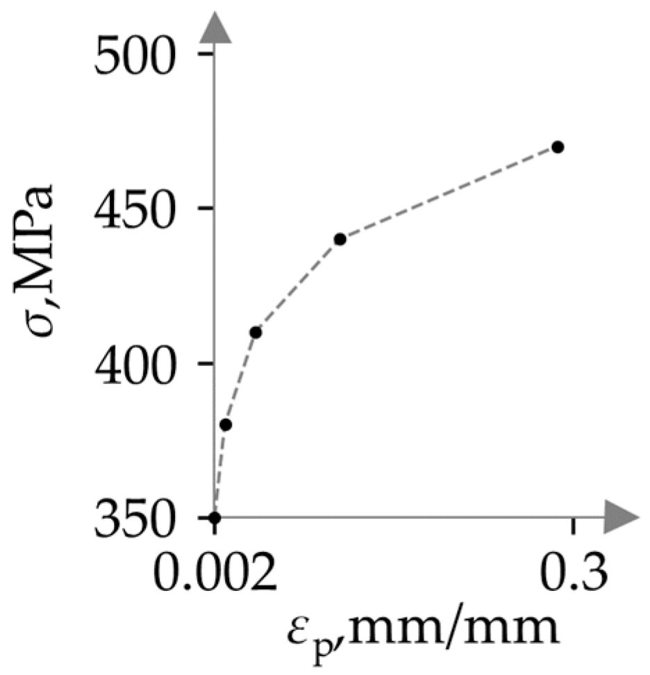
When formulating the multilinear material model in some commercially available finite element analysis software, whether based on one of the mentioned material models or another tailored to a specific material group or loading condition, the calculation of stress values is conducted for specific plastic strain values. The elastic strain is determined using Young’s modulus and Poisson’s ratio. Figure 1 provides an illustrative example of a multilinear curve, defined by five combinations of stress and plastic strain values for incremental selection of stress values in equal steps. The computation of plastic strain values is then performed for each specific stress increment, with the first point conventionally having the stress value equal to yield stress, R_e, or some other designated stress value.

1.2. Problem Definition

A multilinear material model acts as a piece-wise linear approximation of the continuous material curve. Using a more densely selected set of points ensures better alignment to the original curve and, therefore, better accuracy of the resulting stress values obtained from FEA. Especially when modeling components with complex material properties, such as surface-hardened steel components, balancing accuracy with computational efficiency can become important since more complex models take a longer time to complete.

Surface hardening is commonly employed in highly stressed parts of components to enhance their durability and performance. Critical regions are selectively heat-treated to increase their hardness while preserving the integrity and ductility of the rest of the components [11]. For example, metal gear teeth often undergo surface hardening, as they experience cyclic loading that can lead to material fatigue and gear failure [12]. Such materials, possessing gradually varying material properties, are often referred to as functionally graded materials (FGMs) [13]. Surface-hardened gears and surface-hardened components in general exhibit varying levels of hardness, strength, and residual stresses from the surface towards the core, with the exact distribution requiring precise measurement and experimental testing. However, due to the complexities and high associated costs of conducting cyclic experiments, the common approach is to estimate cyclic and fatigue properties from tensile test data or hardness measurements [14,15,16]. Furthermore, the utilization of empirical expressions [17,18] can provide estimations of the hardness distribution across the surface-hardened component, from its outer layer to its core, based on the heat treatment parameters applied during the surface-hardening process. Employing the mentioned estimation techniques to establish correlations between hardness and other material properties enables the comprehensive characterization of the material of such components, which can then be effectively modeled to predict their mechanical behavior.

Significant advances in determining the mechanical behavior of surface-hardened components have been made, from early analytical methods [13,19] to more sophisticated computer-aided numerical methods [12,20]. A widely adopted strategy for the numerical modeling of surface-hardened components, or, more generally, functionally graded materials, is the multilayer method [12,20,21,22], which involves dividing geometry into layers, with each layer characterized by constant homogenous properties. Figure 2 illustrates a typical distribution of Brinell hardness observed in surface-hardened gears with the discretized hardness profile that is then used in FEA to apply the multilayer method.

Regarding the multilayer method, Yin and Fatemi [20] introduced a finite element model to predict the monotonic and cyclic behavior of steel specimens under axial loading. Two models are proposed within the study: a two-layer model and a four-layer model. In the two-layer model, the surface-hardened specimen is divided into a hardened surface and a core, with each layer modeled as a homogeneous material having its own stress–strain curve derived from experimental tests. The four-layer model incorporates two additional layers featuring homogeneous material properties, with each layer characterized by its own stress–strain curves obtained through the interpolation of stress–strain data from the two-layer model.

Similar to the two-layer model mentioned earlier, Yadegari [21] proposed a model to consider the effects of surface hardening in the fatigue strength assessment. The surface layer of the component is modeled as homogenous and exhibits high hardness with an accompanying compressive residual stress state. At the interface to the core of the component, there is an abrupt transition to a homogeneous area of low hardness and tensile residual stress. Using this model, the fatigue life of the component is then calculated based on the local strain approach for the notch root and the point on the interface between the surface layer and core material.

Additionally, Čular et al. [12] proposed a numerical model to predict the location of fatigue crack initiation and the required number of loading cycles for bending fatigue failure in surface-hardened steel gears. The tooth root area of the gears is divided into layers in which constant homogeneous material properties (material strength and residual stress) are assumed to exist within each layer. Only linear FEA was conducted obtaining elastic stresses and strains, which were then corrected for elastoplastic via Neuber’s rule [23]. For fatigue life prediction, the strain-life approach was employed, with the required fatigue parameters estimated using the Hardness method [16].

When the estimation of elastoplastic stresses and strains from elastic strains using approximation methods such as the aforementioned Neuber’s rule is not possible, modeling nonlinear material behavior in finite element analyses becomes necessary. For this purpose, the multilayer method can be employed, which involves assigning each layer its own stress–strain monotonic or cyclic curve using a multilinear material model, as previously mentioned. Modeling each layer with a specific multilinear curve increases the complexity of the finite element model if more stress plastic strain points for each individual curve are used. To keep the complexity of a curve low while still preserving the same compliance to the original curve, the number and position of stress–strain points in a multilinear curve should be selected in an optimal manner.

The problem of optimal discretization of power law-based stress–strain curves has already been explored in the work of Hoff et al. [24]. In this context, a criterion for optimal discretization is introduced with the goal of using the fewest line segments within predetermined error bounds. The proposed formulation results in a system of nonlinear equations with no apparent closed-form solution, requiring solving through an iterative search technique. However, in practical industrial applications, implementing such an iterative approach solely for the discretization of multiple stress–strain curves may be impractical due to time limitations.

The challenge of optimal discretization of stress–strain curves further extends to maintaining consistent accuracy across each individual multilinear curve in relation to the original curve when employing a multilayer approach to model complex material properties. The stress values derived using a multilinear curve can deviate from the ones obtained from the original curve depending on the number and position of multilinear points. Consequently, the resulting stress values obtained from FEA may exhibit inconsistent deviations across the geometry, impacting the overall accuracy and reliability of the model.

Considering all the mentioned challenges, the focus of this research is the optimal discretization of a stress–strain material curve used for defining a multilinear material model. The issue of maintaining a consistent level of compliance to the original curve across multiple multilinear curves is also addressed. Given the considerable time constraints in the industry, the proposed discretization algorithm should require only essential, readily available material parameters.

2. An Overview of Line Simplification Algorithms

As the objective is to optimally select points on a continuous material curve, in this section, various line simplification and curve discretization algorithms are explored. Given a continuous curve, a piece-wise linear approximation is obtained by connecting selected points on a curve with linear segments. Approximation is closer to the original curve by using more optimally distributed points [25]. For a function f(x), piece-wise linear approximation can be obtained for any given value of x′, such that x_i ≤ x′ ≤ x_i+1. The function value f(x′) is then approximated to a combination of f(x_i) and f(x_i+1) [26]. Most algorithms work by first discretizing a continuous curve, which transforms it into a finite set of equally distributed discrete values, thus leading to information loss [27]. A large number of data points that are then acquired is reduced using an algorithm, which decreases the number of piece-wise segments and distributes them in the most favorable position according to prescribed error tolerance, keeping only the most significant points [28]. Different line simplification algorithms can determine the significance of a single data point in different ways, such as by removing the points that are grouped together, measuring the absolute curvature at that point [28], measuring the distance from a selected line segment, and measuring the impact of a point on the overall shape of a line.

2.1. Line Simplification Algorithms and Error Measures

A general proposed division of simplification algorithms is local algorithms, which consider several consecutive original points; global algorithms, which process the whole domain of a function; and independent algorithms, which do not search for any mathematical relationship between neighboring points. An example of a simple independent algorithm is the nth point routine, which selects every fixed number of consecutive points, also called the equal intervals algorithm (EI) [29]. Since the goal is to optimally distribute and select the points to define the multilinear curve, more attention will be given to local and global algorithms.

Local algorithms consider relationships between several neighboring points of a function and decide on the removal of a specific point depending on the distance from other points or the area enclosed by points in its proximity. One such algorithm is the Reumann–Witkam routine [30], which uses user-defined distance tolerance to decide if the point is to be kept or removed. First, a line is defined through the first two consecutive points, x_i and x_i+1. The shortest distance from this line to each next point of the original dataset is calculated, and the points whose distance exceeds the predefined tolerance are kept. The process continues until reaching the last point. The simplification algorithm developed by Lang [29] searches the space of a fixed number of consecutive original points. In the search space, the first and last original points are connected, and the points between them that have a perpendicular distance to that line segment smaller than the tolerance are removed. The Visvalingam Whyatt (VW) algorithm [31] is another local simplification algorithm that works by removing points that cause less change in the shape of the function. Successive triplets of points are formed along the piece-wise function. The algorithm removes point x_i if the area of the triangle with points x_i−1, x_i, and x_i+1 is smaller than the user-defined value. By doing so, the points that give the smallest change in overall function shape are removed, and the iteration starts again [31].

Global line-simplification algorithms consider a relationship between all points of a given dataset in one iteration. Similar to the local Visvalingam Whyatt algorithm, the global VW algorithm [31] also forms successive triplets of points, but computes the effective area of all triangles formed. The algorithm eliminates the point with the minimum effective area in each iteration. This process is repeated, forming successive triplets and removing points until all areas are within the specified tolerance [29].

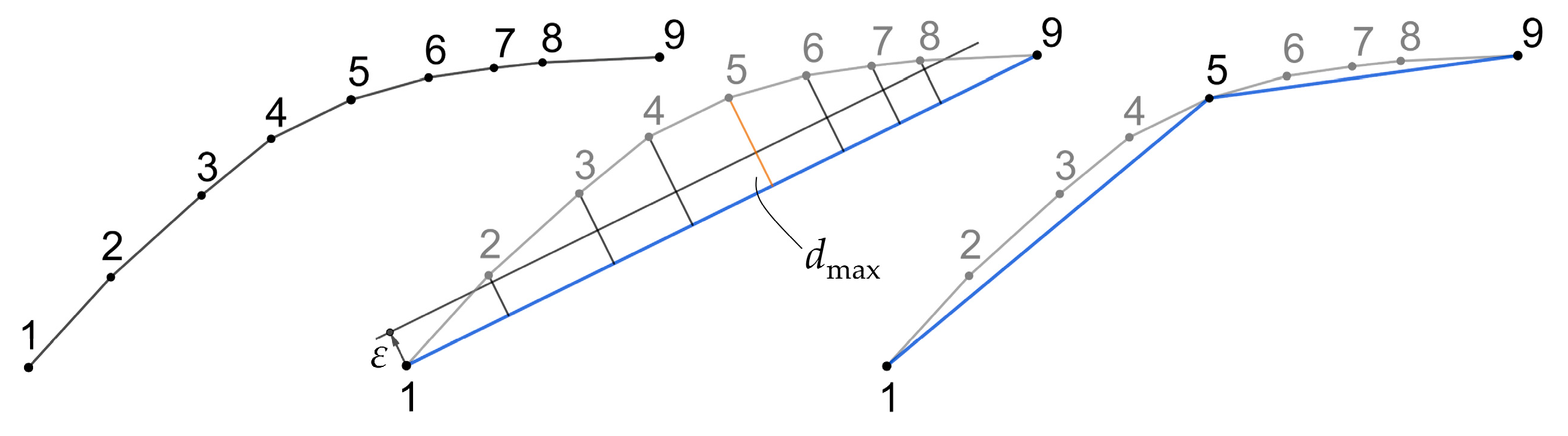
Another example of global simplification algorithm is the Ramer–Douglas–Peucker (RDP) algorithm, shown in Figure 3, which recursively divides the entire line and calculates the distance of points [32]. The algorithm works with an already discretized initial curve by connecting the first original point, x₁, to the last original point of the dataset, x_n, with a line segment and calculating the shortest distances of all original points to that line. The farthest distance is labeled d_max, and the point corresponding to that distance, x_i, is kept in a new simplified dataset if it is outside of the predefined tolerance ε. The iterative process continues with two new line segments, with the point x_i being the new end point for the left line segment and the new start point for the right line segment. The process continues until all points are within the predefined tolerance.

In assessing the accuracy of various line-simplification algorithms [32], the deviation of the discretized polyline from the original shape can be quantified. Deviation of the discretized polyline to the original shape depends on the chosen method and can be quantified measuring the error, taking into account both the number and position of the reduced points. Two commonly employed methods for error calculation are distance-based measures and area-based measures. The positional error sum, a distance-based measure, quantifies positional errors by calculating the distance from the removed points on the original curve to the simplified polyline. Summing the positional errors of every original point results in the positional error sum measure [32], offering a metric for comparing different line-discretization algorithms.

To better understand the global deviation of the simplified polyline from the original, the areal difference measure can be employed [32]. By connecting the first and last points of both the original and discretized polylines, an area is formed. The final error measure is obtained by quantifying both polyline areas and calculating the absolute difference between these areas. Figure 4 illustrates the method for determining the areal difference measure on a polyline similar to the shape of the nonlinear part of a steel stress–strain curve.

These error measures provide valuable insights into the deviation from the original material curve and can serve as an effective stopping criterion when employing simplification algorithms.

2.2. Discussion of the Mentioned Algorithms

The local and global simplification algorithms mentioned earlier work through either point addition or point removal. Initially, a continuous curve is discretized, with points being either removed (VW) or added successively (RDP). Due to this discretization process, the accuracy and final simplified polyline are influenced by the position and density of the original points rather than solely by the complexity of the line [29]. A more effective approach involves directly selecting points from continuous curves, bypassing the need to discretize the initial curve and, thereby, minimizing information loss.

Moreover, the mentioned algorithms rely on user-defined tolerance as a criterion for point removal. For example, the Visvalingam Whyatt algorithm requires the input of minimal triangle size, which is difficult to estimate since the optimal triangle size is not unique and can vary for various material curves to achieve consistent accuracy. Additionally, even slight variations in the tolerance value can lead to different numbers and positions of simplified points on the final polyline. Given that the provided tolerance does not directly indicate the deviation of stresses or strains of the simplified polyline from the original curve and lacks intuitiveness, an alternative stopping criterion must be considered for this purpose.

While the algorithms can be adjusted to stop when a predefined total number of points in a simplified polyline is reached, the desired number of points alone also does not provide meaningful information about the deviation of the simplified polyline from the original curve. That is why incorporating the previously mentioned error measures into the stopping criterion proves to be a more effective approach. The positional error sum depends on the discretization of the original curve, as it sums errors from the original points to a simplified line. Thus, it greatly depends on the number of points in the original curve and the scale of the stresses and strains and cannot be used to compare curves with a different number of points or different material constants. Again, if the positional error sum is a user-defined value, it is difficult to estimate its value, as it does not contain specific information that can be known to the user beforehand. The positional error sum could potentially be useful only in determining the goodness of algorithms when comparing simplified curves with the same number of points obtained from the original curve discretized with an identical number of points.

A better quantifying error measure, which could also potentially be used as a stopping criterion, is the areal difference measure. This measure can be converted to a percentage and used to quantify the percentage that is not explained by the simplified curve. An areal difference measure could be used as a stopping criterion, but it fails to provide information on the maximum deviation of stress values to the original curve, which is information of importance when optimally discretizing a material stress–strain curve. For this reason, another measuring error that considers the deviation of stresses between the simplified and original curves is proposed.

3. Materials and Methods

Considering the assessment and limitations of algorithms in the existing literature, a novel algorithm is introduced for optimizing the discretization of material stress–strain curves. This algorithm incorporates a stopping criterion called the percentage of stress deviation, which is obtained through a maximal vertical distance measure. Unlike the perpendicular distance measure employed in the original RDP algorithm, which calculates the maximal distance from a line segment to a data point on the discretized original curve, the maximal vertical distance measure directly evaluates the maximal vertical distance from the line segment to the non-discretized original curve. This distinction eliminates the need for initial discretization of the material stress–strain curve, thus avoiding additional errors introduced during that process and enhancing the accuracy of the discretization.

3.1. Defining the Maximal Vertical Distance Measure

A maximal vertical distance measure is introduced and implemented to optimally select the points along a material curve for retention. The stopping criterion, defined as a percentage of stress deviation, SD, will be demonstrated using a Ramberg–Osgood material model for illustrative purposes. However, with the necessary adjustments, the stopping criterion and accompanying algorithm can also be applied to other material models.

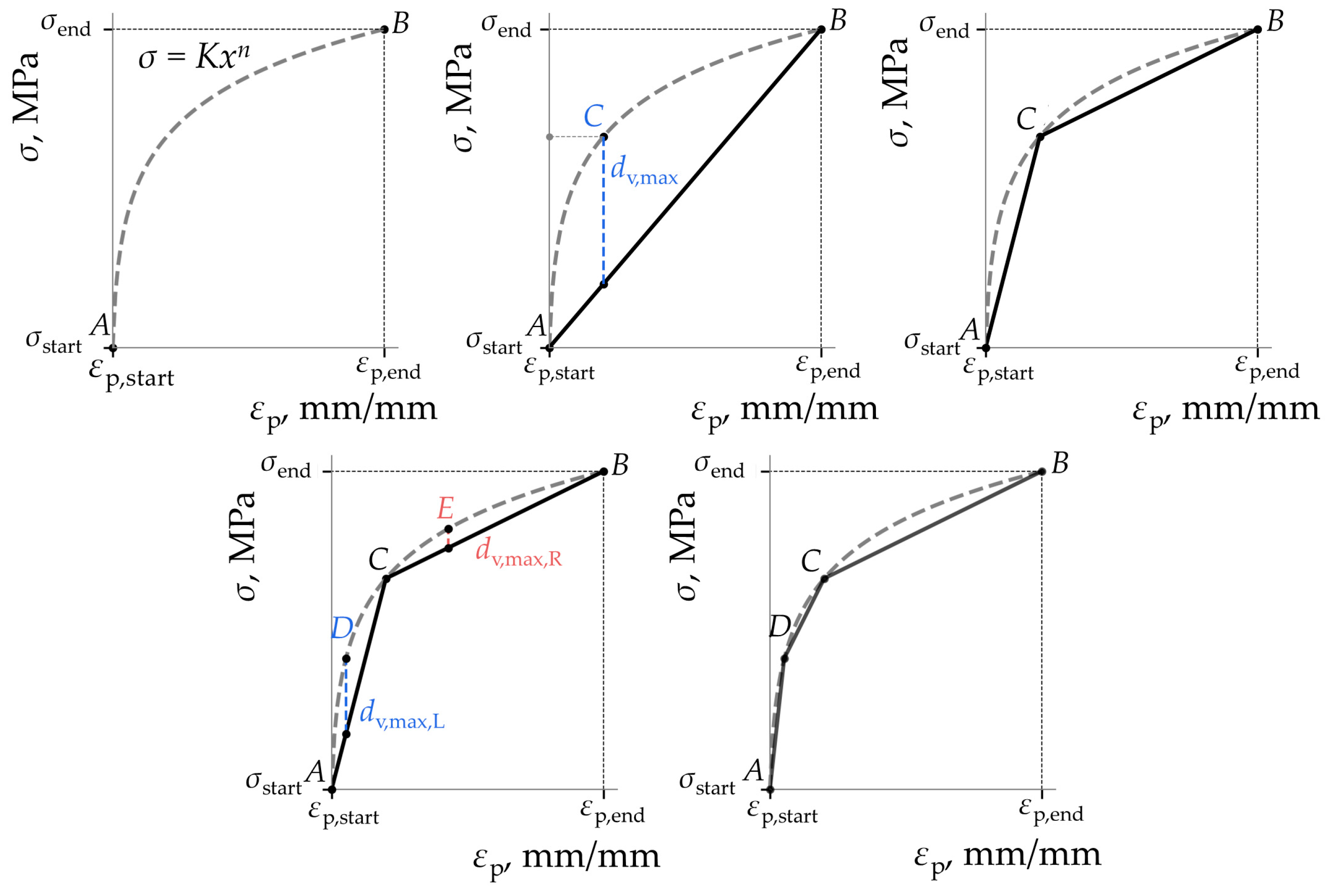
The Ramberg–Osgood model presented in Equation (1) can be further simplified by segmenting the linear and nonlinear portions of the stress–strain curve as follows:

$$\epsilon =\left\{\begin{array}{l}\sigma /E \mathrm{f}\mathrm{o}\mathrm{r} \sigma \le R_{\mathrm{e}}\\ {\displaystyle \frac{\sigma }{E}}+{\left({\displaystyle \frac{\sigma }{K}}\right)}^{{\displaystyle \frac{1}{n}}}\mathrm{f}\mathrm{o}\mathrm{r} \sigma >R_{\mathrm{e}}\end{array}\right..$$

(5)

This form is widely applied in finite element simulations, as it takes advantage of the linearity of the stress–strain relationship before reaching the yield point [33]. Materials display an elastic component of strain both before and after surpassing the yield stress, allowing for the further subdivision of the nonlinear portion of the complete stress–strain curve into elastic and plastic components. The plastic portion of the Ramberg–Osgood curve is a stress–strain power law given by the equation f(x) = Kxⁿ, where x represents plastic strain values and f(x) represents stress values. The strain-hardening exponent, n, has a value between 0 and 1. The strength coefficient, K, is typically defined as the stress value corresponding to a plastic strain value of 100%. To visually demonstrate the maximal vertical distance measure applied to the chosen material model, the stress–strain power law model is presented in Figure 5. This figure shows a line denoted with a function g(x) = ax + b connecting two arbitrary points, A and B, on the material model defined with power law f(x).

As depicted in Figure 6, subtracting the lower line function g(x) from the upper material curve f(x) yields a new function labeled h(x): Kxⁿ − ax − b

$$h\left(x\right)=f\left(x\right)-g\left(x\right)=K{x}^n-ax-b.$$

(6)

If a given function h(x) is differentiable on an interval [a, b], then the maximum value of h(x) in that interval must occur either at x ϵ [a, b], where the first derivative is equal to zero, or at the endpoints a and b of the interval. Thus, the first derivate of this function is:

$$h^{\prime }\left(x\right)=nK{x}^{n-1}-a.$$

(7)

The x_max value for which h(x) is maximized is then obtained by setting the derivative of h(x) to zero:

$$\begin{gathered} nK{x}^{n-1}-a=0, \\ {x}_{\mathrm{m}ax}={\left({\displaystyle \frac{a}{nK}}\right)}^{{\displaystyle \frac{1}{n-1}}}. \end{gathered}$$

(8)

The maximal vertical distance between the line segment g(x) and the material curve f(x) is calculated by substituting x_max (Equation (8)) into the function h(x) (Equation (6)):

$$\begin{gathered} d_{\mathrm{v},\mathrm{m}\mathrm{a}\mathrm{x}}=K{x}_{\mathrm{m}\mathrm{a}\mathrm{x}}^n-a{x}_{\mathrm{m}\mathrm{a}\mathrm{x}}-b, \\ {d}_{\mathrm{v},\mathrm{m}\mathrm{a}\mathrm{x}}=K{\left({\displaystyle \frac{a}{nK}}\right)}^{{\displaystyle \frac{n}{n-1}}}-a{\left({\displaystyle \frac{a}{nK}}\right)}^{{\displaystyle \frac{1}{n-1}}}-b. \end{gathered}$$

(9)

Figure 7 illustrates the process of obtaining the maximal vertical distance between a continuous curve given by a power law and a line segment.

The resulting maximum vertical measure (d_v,max) is then normalized by the stress value corresponding to the strain value for the maximal vertical distance, denoted as σ_max. This yields a measure used as a stopping criterion in the proposed algorithm called the percentage of stress deviation (SD), with the formula defined as:

$$SD={\displaystyle \frac{d_{\mathrm{v},\mathrm{m}\mathrm{a}\mathrm{x}}}{{\sigma }_{\mathrm{m}\mathrm{a}\mathrm{x}}}}\cdot 100.$$

(10)

When using an alternative material model defined by a different constitutive equation, it is essential to integrate the relevant parameters and functional expressions, along with their derivatives, into the presented framework. If the chosen alternative material model is complex and the exact computation of its first derivative requires numerous function evaluations, the utilization of numerical differentiation algorithms becomes needed for approximating the derivative.

The proposed maximal vertical distance measure, along with the percentage of stress deviation, offers a comprehensive and intuitive approach for optimizing the discretization of the Ramberg–Osgood power law for use in a multilinear material model.

3.2. Proposed Maximal Vertical Distance Recursive Algorithm (MVD)

The percentage of stress deviation (SD) is implemented into the algorithm for optimal point selection from the continuous material curve, using the plastic portion of the Ramberg–Osgood model (stress–strain power law) as an example. This implementation refines the original Ramer–Douglas–Peucker (RDP) algorithm, which relies on maximal perpendicular distance for point retention by adopting the previously explained maximal vertical distance measure. By doing so, the need to discretize the initial curve is eliminated, ensuring that the accuracy of the resulting simplified polyline remains independent of the number of discretized points originally present on the curve. This represents a significant advantage over existing algorithms like RDP and VW, as documented in the literature. Furthermore, this approach provides precise insights into the stress deviation of the multilinear curve in relation to the original Ramberg–Osgood curve, with the measure of SD serving as the algorithm’s stopping criterion.

The proposed algorithm is implemented on the plastic portion of Ramberg–Osgood material model and is designed to request user-input values, including the following:

• The coefficients used to describe the Ramberg–Osgood material curve: the strength coefficient (K) and strain-hardening exponent (n) in the case of static loadings, and the cyclic strength coefficient (K′) and exponent n′ in the case of cyclic loadings;
• The minimum plastic strain value (ε_p,start) at which the first corresponding stress value is calculated, typically set at 0.2%;
• The maximum desired plastic strain (ε_p,end);
• The desired percentage of stress deviation (SD_lim).

The pseudo-algorithm for the proposed maximal vertical distance recursive algorithm (MVD) applied to the plastic portion of Ramberg–Osgood material model is outlined in Algorithm 1.

Algorithm 1. Pseudo-algorithm of the maximal vertical distance (MVD) recursive algorithm.
Input variables: K (or K′), n (or n′), εp,start, εp,end, SDlim.
With σstart = Kεnp,start define start point A (σstart, εp,start). With σend = Kεnp,end define end point B (σend, εp,end).
Define function: MVD (K, n, A, B, SDlim)
	Connect start point, A with end point, B and calculate linear equation coefficients of formed line.
	Calculate the maximal vertical distance and select the point C on material curve for which maximal vertical distance is reached.
	Calculate percentage of stress deviation, SD.
	If SD > SDlim:
		Recursive call:
		MVD (K, n, A, C, SDlim) MVD (K, n, C, B, SDlim)
	Else:
		Keep the points selected until this step.

The outlined method is visually depicted in Figure 8, utilizing the following material constants of low-alloy steel taken from [34]: K = 549 MPa, n = 0.038, conventionally taken ε_p,start = 0.002, and a maximum stress deviation SD_lim = 5%. Initially, the algorithm defines a starting point A (σ_start, ε_p,start) and an end point B (σ_end, ε_p,end), with R_e and σ_end computed using the plastic portion of the Ramberg–Osgood equation (Equation (5)) for corresponding values of stress. Subsequently, the algorithm establishes a line connecting points A and B by determining the coefficients of the linear equation that characterize this line.

Utilizing the maximal vertical distance measure, the algorithm computes the maximum vertical distance, d_v,max, from this line to the material curve, characterized by constants K and n. A new point, C, is then marked on the curve. The stress on the material curve corresponding to the strain value of the maximal vertical distance, denoted as σ_max, is used to calculate the stress deviation (SD). If the stress deviation (SD) exceeds the predefined limit of maximum stress deviation (SD_lim), point C is retained as a new point on the simplified polyline. The algorithm then divides the material curve into left and right sides from point C. It then recursively calls itself, computing the maximal vertical distance and, consequently, the percentage of stress deviation for the two new line segments, $\overline{AC}$ and $\overline{CB}$, denoted as d_v,max,L and d_v,max,R, respectively. Recursion concludes when the percentage of the stress deviation of the constructed polyline (SD) computed from the maximal vertical distance falls below the user-defined value (SD_lim).

4. Results of Comparison of Proposed MVD Algorithm with Existing Algorithms

The proposed maximal vertical distance recursive algorithm (MVD), as illustrated in the Ramberg–Osgood model, is compared with two algorithms, one being the global Visvalingam Whyatt (VW) algorithm [31] and other one being an independent equal-intervals algorithm (EI) [29], both mentioned in Section 2.1. Adjustments were made to the original VW algorithm to ensure that it generates a simplified polyline with the same number of points as obtained from the MVD algorithm. This ensures a fair comparison, focusing solely on the accuracy of the resulting polylines in regard to the original material curve, eliminating the variable of a different number of points on a simplified polyline, which can result in different computing times when loading the multilinear curve to the finite element model.

The VW algorithm computes the area of triangles formed by three successive points on the initial curve. This necessitates the discretization of the initial material curve, leading to potential variations in the position of points on the final simplified polyline based on the initial discretization. The VW algorithm requires user-input values, including the material constants of the used-material model, the number of initial discretization points, and the desired number of final points on the simplified polyline. Starting with the material constants, the material curve is initially discretized to a specified number of points. In each iteration, the algorithm calculates the minimal triangle area from the first to the last point. The middle point of the triangle with the minimal area is then removed, and the next iteration proceeds with all points except the removed one. The algorithm stops when it attains the desired number of points on a simplified polyline. Ultimately, the percentage of the stress deviation (SD_fin) of the constructed polyline is computed in relation to the original material curve.

The EI algorithm, on the other hand, simply selects a fixed number of consecutive points with equal intervals based on strain and also maintains an equivalent number of points to the MVD algorithm for the sake of comparison.

The comparative analysis of the MVD, VW, and EI algorithms is presented in

Table 1. Comparison of MVD, VW, and EI algorithms on different materials.

Stopping Criterion	Algorithm	Number of Initial Points	K = 549 MPa n = 0.038 εp,start = 0.002		K = 1435.7 MPa n = 0.276 εp,start = 0.002
			SDfin, %	Final Number of Points	SDfin, %	Final Number of Points
SDlim = 2%	MVD		1.1	5	1.9	9
Number of simplified points *	EI		0.8		3.18
	VW	500	2.49		5.05
	VW	1000	2.52		5.29
	VW	10,000	2.02		3.24
SDlim = 5%	MVD		4.57	3	4.57	6
Number of simplified points *	EI		2.85		6.65
	VW	500	5.94		12.69
	VW	1000	5.94		12.82
	VW	10,000	5.38		10.46

* The VW and EI algorithms stop when the same number of simplified points that were obtained with MVD algorithm are reached.

and is conducted on the plastic portion of Ramberg–Osgood material model with a starting strain value of 0.2% and final strain value of 30% for illustrative purposes. During the generation of simplified points through the MVD algorithm, two SD limits, 2% and 5%, were investigated. The resultant number of final simplified points obtained from the MVD algorithm was then employed as a stopping criterion for both the VW and EI algorithms.

For the VW algorithm, the initial plastic portion of the Ramberg–Osgood curve underwent discretization by generating equally spaced strain values between the starting and final strain values. To evaluate the VW algorithm’s performance under different levels of discretization, the discretization of the initial Ramberg–Osgood curve was performed using different numbers of initial points: 500, 1000, and 10,000. Using the EI algorithm, stress values were also computed from the plastic portion of the Ramberg–Osgood curve at equal intervals of strain values, corresponding to the number of points obtained from the MVD algorithm.

This systematic procedure was repeated for two distinct steel materials, each characterized by different Ramberg–Osgood monotonic material constants. These constants cover a wider range and are obtained from experimental tests from the available literature. The first studied material is characterized by K = 549 MPa and n = 0.038 [34], and the second material by K = 1435.7 MPa and n = 0.276 [35]. Subsequently, the final SD_final measure for each simplified line was determined and is presented in Table 1.

The proposed maximal vertical distance algorithm performs better than the Visvalingam Wyatt algorithm in terms of the finally obtained stress deviation percentage (SD_fin) for all combinations of studied material constants and maximal stress deviations (SD_lim). For different numbers of initially given points, the discretized polyline obtained from the Visvalingam Wyatt algorithm obtains varying SD_fin measures, making it less reliable. When comparing the obtained SD_fin values with the maximal requested limit SD_lim, the VW algorithm yields values exceeding the limit for the same number of points as those obtained by the MVD algorithm. Determining the optimal number of initial discretization points for the VW algorithm is challenging, given the variability in SD_fin limits. Also, a considerable number of points is needed for the discretized polyline to closely resemble the original curve. As the VW algorithm iteratively removes points starting from the complete set, it demands a greater computational effort with finer initial discretization.

The equal-intervals algorithm occasionally exhibits a lower percentage of stress deviation compared to the MVD algorithm. However, it is inconsistent, as it does not comply with the limit of stress deviation in every observed case, making predictions unreliable. In contrast, the MVD algorithm stops once it achieves the minimum number of points required to meet the stress deviation criterion, ensuring consistent adherence to predefined limits.

To visually illustrate the multilinear curves obtained using the compared algorithms, only specific parameter combinations from Table 1 were chosen. Here, the focus is on results corresponding to SD_lim of 5% and a fixed number of initial points for VW discretization set at 10,000. This visual representation includes both materials and all three algorithms and is depicted in Figure 9, with the left side illustrating material 1 and the right side illustrating material 2. The upper graphs showcase the final multilinear curves obtained from all algorithms, while the bottom graphs illustrate the percentage of stress deviation, SD, obtained for the values of the plastic strain. Notably, the peaks of stress deviation (SD_fin) are most pronounced at smaller values of plastic strains.

It is evident from the figure that the EI algorithm can occasionally yield even lower values of SD_fin than the MVD algorithm, particularly notable for material 1. However, since it exceeds the limit of stress deviation for material 2, it is clear that it is failing to adhere to the initial condition. To keep the EI algorithm within the predefined limits, a greater number of points would be required, which would increase model complexity. Although the MVD algorithm may appear visually farther from the Ramberg–Osgood line for material 2, it is important to note that it guarantees all stress values calculated from strain values during finite element analysis will remain within the predefined limits. This level of reliability is not ensured with the EI and VM methods, which may exceed limits depending on specific combinations of parameters, making them overall less consistent.

The MVD algorithm holds a distinct advantage by directly selecting points from the original Ramberg–Osgood curve, characterized by parameters K and n, thereby eliminating the need for initial discretization. Furthermore, with the methodical approach of starting with only two initial points and systematically adding one at a time, the MVD algorithm exhibits fast computing times. On the other hand, due to its straightforward method of selecting equal intervals of points and calculating corresponding stress values, the EI algorithm exhibits faster performance than MVD on average. It is indeed possible that EI could achieve better SD_fin performance if given the same time as MVD. Despite this speed advantage, the results remain favorable for MVD due to conducting the simultaneous optimization. The EI algorithm might densely allocate points in areas already within the SD_lim measure, resulting in an unnecessarily high number of points, while the approach to use fewer points is prioritized, as discussed in Section 1.2. In comparison to VW, which also performs optimization, the MVD algorithm exhibits significantly faster performance.

5. Application of the MVD Algorithm and Discussion

This section addresses the challenge of generating multilinear curves to characterize surface-hardened steel, as discussed in the introduction. When simulating surface-hardened components in finite element analysis (FEA), the aforementioned multilayer approach, which segments the geometry into layers and applies homogeneous properties to each layer, proves effective [12].

To illustrate the generation of multilinear curves for fatigue analysis of surface-hardened components using the MVD algorithm, AISI 4140 or 42CrMo4 low-alloy steel is chosen due to its widespread use in machinery and automotive engine applications [11]. After undergoing heat treatment, this steel exhibits desirable properties such as high fatigue strength and wear resistance.

For the purpose of illustrating the generation of multiple multilinear curves, the typical hardness profile of surface-hardened components is discretized into five layers, each with uniform hardness distribution (Figure 2) and represented with one multilinear stress–strain curve. To generate a distinct multilinear curve for each layer, equations correlating hardness measurements taken at various cross-section points with Ramberg–Osgood cyclic material parameters are utilized. In the literature, a strong correlation between the cyclic strength coefficient K′ and hardness is identified, while a good correlation between hardness and the cyclic strain-hardening exponent n′ is absent [15,36]. Consequently, a regression equation correlating cyclic strength coefficient K′ with Brinell hardness HB of 42CrMo4 steel is employed, while the strain-hardening exponent n′ is taken as a constant value [15]:

$$\begin{gathered} K^{\prime }=0.009H{B}^2+0.1173HB+376.75, \\ {n}^{\prime }=0.1087. \end{gathered}$$

(11)

Arbitrarily selected hardness values ranging from 550 HB (surface) to 420 HB (core), as observed in the distribution shown in Figure 2, are employed to represent a surface-hardened component. From these hardness values, using Equation (8), the cyclic strength coefficient K′ is calculated, and the cyclic strain-hardening exponent n′ is constant. The conventional starting point of the plastic strain, ε_p,start = 0.002, is chosen, from which the yield stress R_p0.2 is determined.

The proposed MVD algorithm, characterized by a predetermined stress deviation value SD_lim, ensures that each layer’s multilinear curve adheres to the specified stress deviation threshold. This way, the accuracy of stress amplitudes for any observed strain amplitude remains consistent regardless of the geometry’s position.

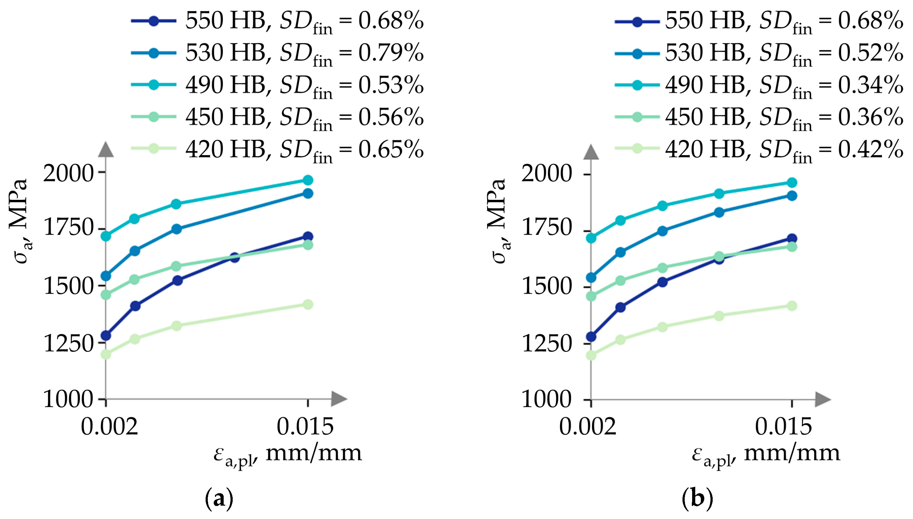
Figure 10 provides multiple multilinear curves constructed for the selected hardness values with the maximum predefined stress deviation SD_lim of 1% and maximum plastic strain amplitude of 0.015 mm/mm (1.5%). Subsequent calculation of the final stress deviation from the original Ramberg–Osgood curve for each multilinear curve reveals a consistent SD_fin of 0.82% across all curves, confirming the adherence to the specified stress deviation threshold. Each multilinear curve comprises five points, discretized at equal strain intervals.

When the strain-hardening exponent is not held constant, the resulting multilinear curves may display varying slopes and potentially overlap. Consequently, not all curves will share the same optimal strain values. This variability can pose challenges, particularly in FEA, wherein convergence issues may arise due to differing intervals of strain values between multilinear curves [37]. When modeling temperature-dependent materials, the same challenge arises wherein each temperature level requires its own material curve, similar to the situation with varying hardness levels, wherein each hardness level necessitates its own material curve [37]. Thus, the approach of achieving uniform strain distribution across multiple curves, as discussed, can be similarly applied to temperature-dependent materials to ensure consistency and reliability in simulations across different temperature ranges.

To illustrate the aforementioned situation of generating multiple multilinear curves with varying strain-hardening exponents, the following regression equation between the strain-hardening exponent (n′) and the ratio of yield stress to ultimate strength (R_e/R_m), valid for most steels, serves as an example [38]:

$$n^{\prime }=-0.33\left({\displaystyle \frac{R_{\mathrm{e}}}{R_{\mathrm{m}}}}\right)+0.40.$$

(12)

As the regression equation does not directly associate the cyclic strain-hardening exponent with hardness, regression equations correlating yield and ultimate strength to Brinell hardness are used, which are valid for 42CrMo4 low-alloy steel [32]:

$$\begin{gathered} R_{\mathrm{e}}={\displaystyle \frac{354.6-0.517HB}{1-\left(\frac{HB}{291}\right)+{\left(\frac{HB}{568}\right)}^2}} \\ {R}_{\mathrm{m}}={\displaystyle \frac{H{B}^2}{400}}+1.6HB+270. \end{gathered}$$

(13)

Using Equations (11)–(13), multilinear curves are generated, as illustrated in Figure 11a. It is evident that each curve is optimized independently, resulting in varying strain intervals between curves and differing numbers of points. However, despite these variations, all curves remain within the prescribed 1% stress deviation limit. This demonstrates the MVD algorithm’s ability to optimize each individual curve separately while maintaining overall adherence to the specified stress deviation threshold.

If requiring all curves to share identical discrete strain values, one approach could be to first identify the curve with the highest number of individual discretized points. If multiple curves have the same number of points, the curve with the lowest stress deviation SD_fin is chosen. Finally, the discretized strain values from the selected curve should be applied to discretize all others. In this specific case, the curve with a hardness value of 550 HB had the greatest number of points, which was 5. The discretized strain values obtained from this curve were, therefore, used to discretize all other curves. Consequently, the multilinear curves illustrated in Figure 11b were obtained. It is evident that all multilinear curves remained within the initially defined stress deviation limit of 1%. This process ensures uniformity in strain distribution across all multilinear curves, as well as the consistency and accuracy of modeling the material at different hardness levels.

6. Conclusions

The maximal vertical distance (MVD) recursive algorithm presents a robust and efficient method for the optimal discretization of the material stress–strain curve, as is demonstrated in the stress–strain power law. Such discretized material curves can then be employed in finite element analysis software describing the material behavior of a component under consideration using the multilinear material model. By directly selecting points from the material curve, the algorithm eliminates the need for initial discretization, ensuring consistent compliance with the original curve across multiple multilinear curves.

Comparative analysis with the Visvalingam Whyatt (VW) and equal-intervals (EI) algorithms highlighted the MVD algorithm’s consistency in accuracy regarding the percentage of stress deviation (SD). The MVD algorithm outperformed the VW algorithm in terms of the final stress deviation percentage (SD_fin) for all studied parameter combinations. Additionally, the VW algorithm failed to maintain SD_fin within an initially set percentage of stress deviation (SD_lim) for some parameter combinations. The EI algorithm, while occasionally exhibiting a lower SD_fin than the MVD algorithm, proved unreliable and inconsistent, as it often failed to adhere to the initial condition of SD_lim. Only the MVD algorithm guarantees that the final percentage of stress deviation (SD_fin) will remain within the predefined limits (SD_lim) for any combination of input parameters, ensuring that all possible stress values during the execution of finite element analysis will be within the specified limits.

Additionally, its simplicity, efficiency, and ability to maintain accuracy across various multilinear curves, as shown in Section 4, make it valuable for simulating components with complex material properties in finite element analysis.

Future investigations will involve the development of a parametric numerical model, enabling the efficient testing of different material states after surface-hardening with material curves defined using the MVD algorithm. Given the complex properties of surface-hardened components and the associated challenges of finite element modeling, future work aims to enhance the reliability and precision of simulations concerning the mechanical behavior of these materials.