Abstract
A dump is a loose accumulation of solid waste from mining operations that easily leads to disasters such as landslides and debris flows. Taking a dump in the Panzhihua region of China as an example, based on the MPM and SPH meshless methods, the dynamic calculation of the instability process of the spoil slope was carried out according to the realistic three-dimensional calculation model of the generated terrain. Firstly, the strain and displacement of the dump under normal conditions and heavy rainfall conditions were simulated by the MPM material point method. The maximum spatial displacement of the dump under heavy rainfall conditions reached up to 386 m. Then, the motion and morphology of the accumulation of the dump under ordinary working conditions and heavy rainfall conditions were analyzed using the smooth particle hydrodynamics (SPH) method. Under heavy rainfall conditions, the maximum horizontal displacement of the dump was approximately 394 m. The research results are conducive to the risk assessment of the spoil slope and provide theoretical support for the calculation of the range of potential threats from the dump.
1. Introduction
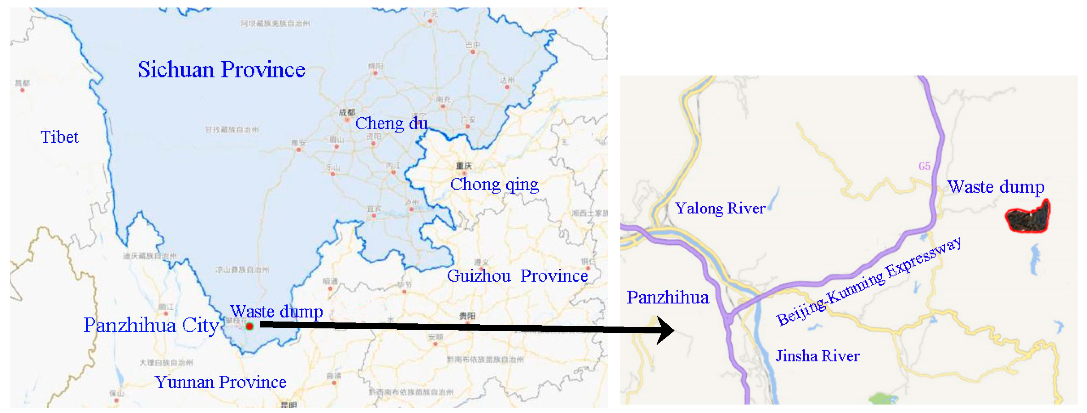
A dumping site refers to a place where waste soil, waste rock, waste residue, and other wastes are concentrated and discharged from mining operations. Generally, it contains a very large volume of waste material. Because it is an artificial loose accumulation of material, a dumping site often presents potential safety hazards that are affected by various factors. Without reasonable support measures, it can very easily deform and lose stability. Landslides, debris flows, and other disasters not only affect the normal production of mines but also pose serious threats to the lives and property of citizens and can damage the environment. For example, in October 1966, in the small village of Aberfan in southern Wales, the United Kingdom, a landslide occurred in a waste pile; it is known as the “everlasting pain in the history of Wales” mine disaster of the village of Aberfan. After several weeks of rain, coal mine waste soil was severely liquified into thick mud that flowed down steep slopes at more than 128 km per hour, killing 144 people, including 116 school children. On 30 April 2006, a dam-break landslide accident occurred when Zhen’an County Gold Mining Co., Ltd. of Shangluo City, Shaanxi Province increased the capacity of its tailings dam. The amount of tailings sand released was about 200,000 cubic meters; 76 residential houses were destroyed, 22 people were buried, 5 people were rescued, and 17 people were missing. On 22 February 2023, a large-scale landslide occurred in the Xinjing Coal Mine in Inner Mongolia. More than 50 operating vehicles were working at the bottom of the pit. The workers and vehicles at the bottom of the pit were buried instantaneously, resulting in 53 deaths and six injuries. The direct economic loss was CNY 204 million. In June 2017, a landslide occurred at a coal mine north of Athens in the northern region of Greece. Approximately 80 million cubic meters of earth and rock were displaced, causing damage to houses and evacuation of villagers, resulting in the burial of at least 25 million tons of lignite and losses of up to EUR 500 million. On 28 February 2022, a landslide occurred again in the Pagan Jadeite mining area in Kachin State, northern Myanmar. At the time of the incident, three excavation groups were on-site, with about 12 people in each group. In addition, there were more than ten maintenance personnel on the site. After the landslide, more than 50 workers on the site disappeared, and three excavators and a truck were also buried. Landslides are due to natural phenomena and human-induced waste dumps. Natural phenomena include earthquakes, rainfall, snowmelt, floods, surface water erosion, soaking, rivers, other surface water on the slope toe of the continuous erosion, etc. Human-induced waste dumps include, for example, unreasonable human activities, excavation of slope toe, blasting, violation of mining sequence, indiscriminate excavation, lack of professionals in some design units, poor location of reservoir site selection leading to dam foundation subsidence, violation of design construction, an illegal increase of loading, and improper safety evaluation of existing problems, all of which ultimately lead to the occurrence of accidents. Therefore, it has become a nonnegligible problem to study the stability of mine dumps and predict the range of possible risks from a collapse accident.
A dump is a deposit formed by stacking materials, and it is characterized by particle size classification and particle breakage. Its stability is affected by many factors, such as the mechanical properties of the deposit, rainfall, earthquakes, external loads, bearing capacity of the foundation, slope gradient and height, topography, surface vegetation, and gully surface runoff. There are roughly three types of factors: the physical and mechanical properties of the deposit, the bearing capacity of the foundation of the dump, the design of the dump, and the stacking process. For example, Rajak studied the effects of different slope heights, slopes, and soil materials on the stability of dumps [1]. Some scholars analyzed the stability of the dump based on the mechanical parameters, stacking sequence, and substrate properties of the dump deposit, and some scholars studied the failure mode of dump slopes and claimed that there are two modes of landslides, traction landslides and push landslides in the dump.
The main research methods of dump slope stability are numerical simulation analysis and model test analysis. The rigid body limit equilibrium analysis method, which originated from the rigid body limit equilibrium analysis method based on statistics, has been proven to be accurate by many projects at home and abroad, but it cannot reflect the changes in stress and strain of the slope with time. With the rapid development of computers, the finite element method and finite difference method based on elastic–plastic theory, usually combined with the strength reduction method, are widely used in slope stability calculations. For example, Gupta combined with strength reduction method, and a stability analysis of the dump slope structure based on numerical simulations was performed [2]. Omracia used the finite element method to calculate the stability of a dump and analyzed the influence of different materials on the deformation of the slope [3]. Rai used the finite difference method to calculate the stability of the dump [4]. There are also discrete medium mechanics methods and meshless methods for large deformation, such as the discrete element method (DEM), discontinuous deformation analysis method (DDA), smoothed particle hydrodynamics method (SPH), and material point method (MPM). The discrete element method is a numerical analysis method proposed by Cundall and applied to the stability analysis of rock and soil. Quezada J. C. analyzed the global stability of mine waste dumps by means of discrete element simulations [5]. Due to the limitation of grids, the calculation is likely to be nonconvergent. Therefore, some meshless numerical methods are used in the analysis of large deformation problems, such as the smoothed particle hydrodynamics (SPH) method and the material point method (MPM) [6]. The material point method is a new particle-type numerical method that combines the advantages of Lagrangian and Eulerian algorithms. It was proposed by Sulsky and has been widely used to simulate the whole process of landslide failure [7,8,9,10,11,12,13]. Smoothed particle hydrodynamics is a numerical method proposed by Ginold and Monaghan [14]. It describes a continuous fluid (or solid) as a group of interacting particles. Each material point has a variety of physical quantities, including mass and velocity. By solving the dynamic equation of the particle group and tracking the trajectory of each particle, the mechanical behavior of the whole system is obtained. The SPH method is a meshless method based on the Lagrangian description [15,16,17,18]. It has been widely used in the simulation of landslide and debris flow disasters [19]. Bui applied SPH to the elastoplastic relationship of rock and soil and then combined it with the strength reduction method to simulate the slope stability [20,21].
Quantitative prediction of the dynamic evolution process of geological disasters is an important basis for solving the risk range of disasters and conducting risk assessments. This study takes a dump in Panzhihua as an example (Figure 1). Based on the MPM and SPH methods, the movement and accumulation of the dump slope after instability under different working conditions were simulated and predicted. The key parameters such as transportation speed, migration range, and accumulation thickness were calculated, and the displacement of the waste calculated by the two methods was comprehensively considered and analyzed. The final range of the potential threat of the dump was thereby realized. The research results are conducive to the risk assessment of the spoil slope.

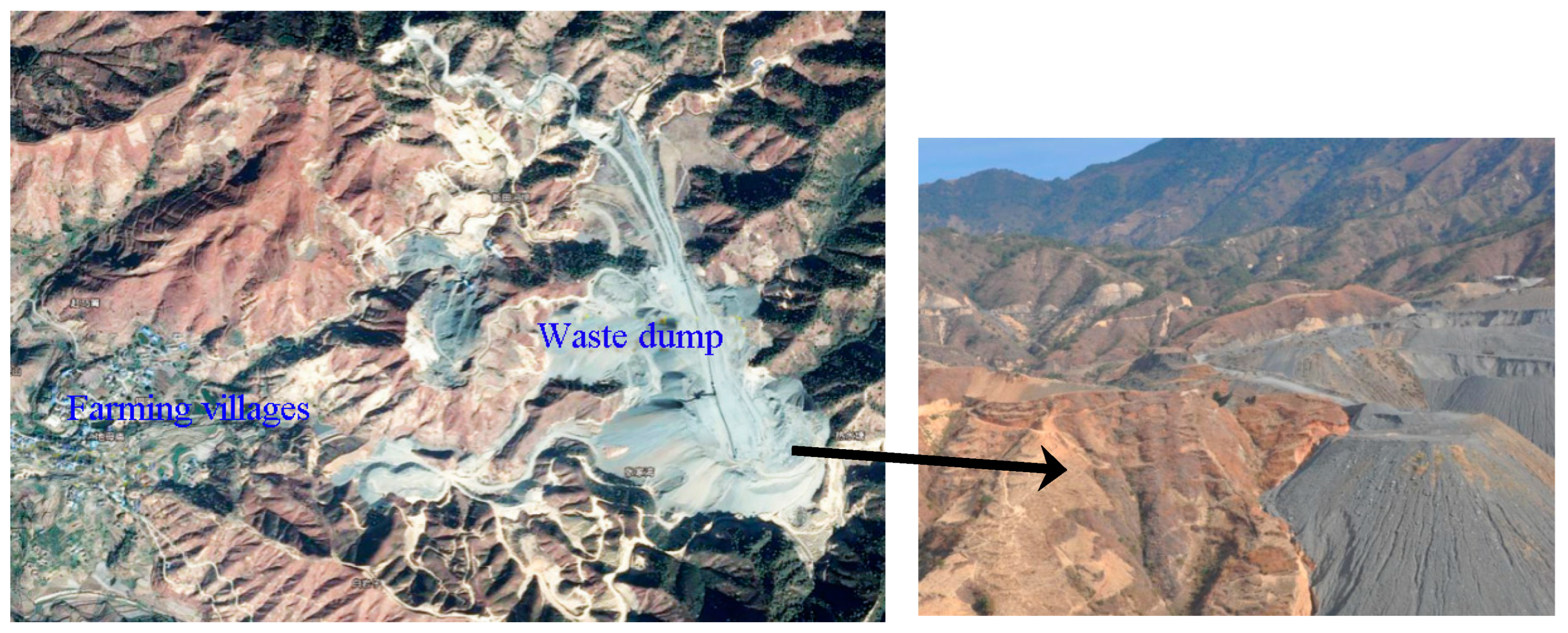
Figure 1.
Geographical location of the study area.
2. Research Area Overview
The dump is located around an open pit mine. The overall landform belongs to the middle mountain area of tectonic denudation, and the microtopography is developed with ridges and valleys (Figure 2). The terrain fluctuates greatly, and the stop and dump are in the operation stage. The natural slope of the ground at the site is generally 20~45°, and the local slope is 70°. The vegetation in the field area is not developed; there are few trees on the top and slope of the mountain, and most of the slope toe and river valley have been transformed into farmland. The gullies in the field area are developed, and the gully trend is basically consistent with the slope tendency. The ground elevation of the dump is between 1561.97 and 1757.06 m, and the relative height difference is approximately 195.10 m.
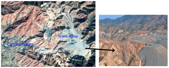
Figure 2.
Topographic and geomorphological characteristics of the dump.
The dump stratum mainly includes a Quaternary Holocene artificial accumulation layer (Q4ml), which is composed of cohesive soil, mixed sand, and broken (block) stone. It consists of the soil and stone that were abandoned during strip mining in the area, mainly distributed in the land section. The Quaternary Holocene alluvial–proluvial layer (Q4al+pl) is muddy silty clay, coarse sand, and a small amount of round gravel, broken stone, cohesive soil, and drift (pebble) stone (mainly composed of granite), which are distributed in the section where there is a gentle slope at the ditch mouth of the dumpsite. In the Quaternary Holocene slope alluvial layer (Q4dl+pl), the silty clay is brownish yellow and brownish red, and it is mainly distributed in the foothills and slopes of the dumpsite. The bedrock stratum of the dump is mainly granite (γ) (Figure 3), which is buried shallowly or partially exposed to the surface. The overburden is weathered granite, and the waste is mainly granite particles, namely massive slag, containing a small amount of fine particles.
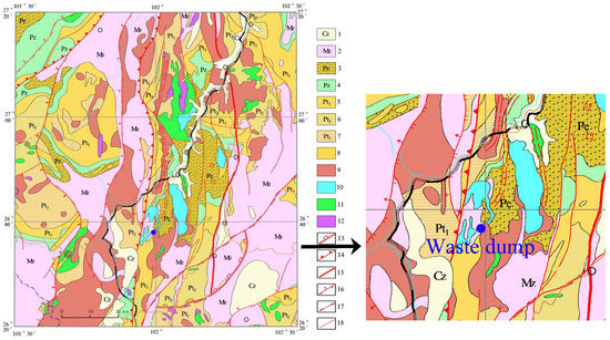
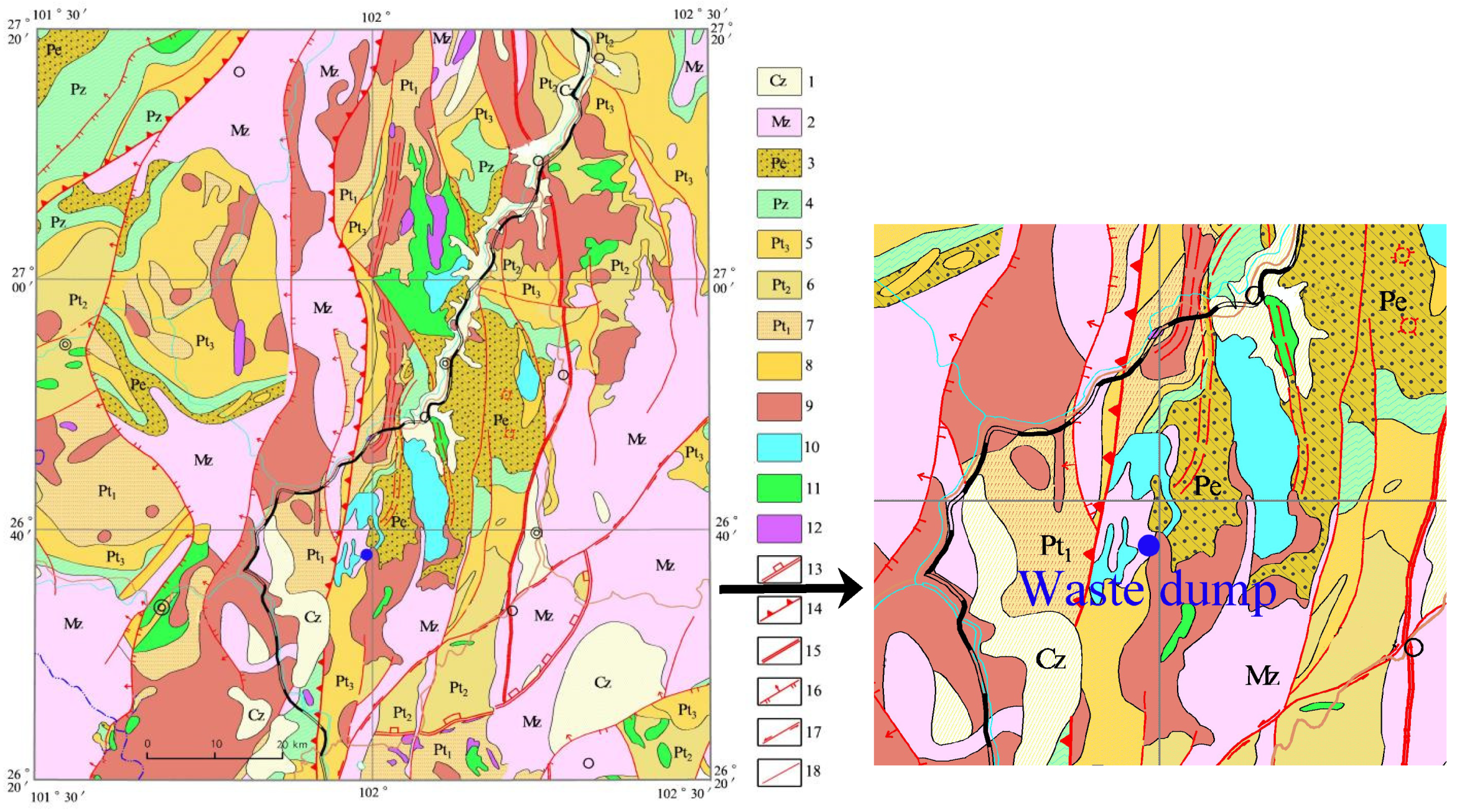
Figure 3.
Geological map of the study area. 1—Cenozoic; 2—Mesozoic; 3—Emeishan basalt; 4—Paleozoic; 5—Upper Proterozoic; 6—Middle Proterozoic; 7—Lower Proterozoic; 8—alkaline rock; 9—acid rock; 10—neutral rock; 11—basic intrusive rock; 12—ultrabasic rock; 13—a plate junction zone; 14—a thrust nappe fault; 15—main composite fault; 16—a reverse fault; 17—flat thrust fault; 18—unknown fault.
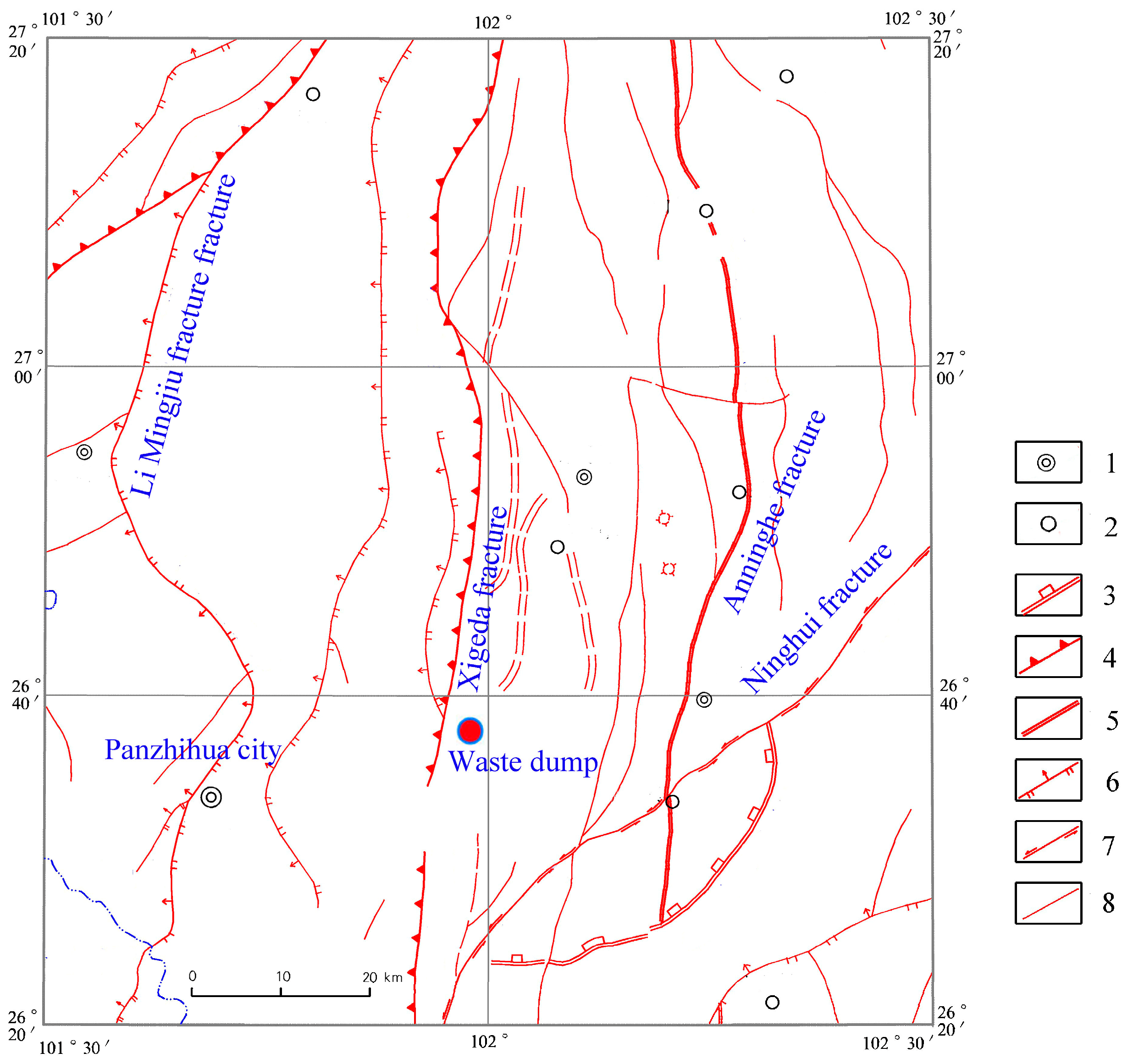
The study area is located in the middle of the north–south tectonic belt in the southern Sichuan and Yunnan Provinces. The structure in the area is complex, the folds and faults are developed, and the whole area is developed. The north–south and north–north-east compression–shear fault structures are the main structures. The north–south structure is represented by the Xigeda and Anninghe faults, and the most influential fault is the Xigeda fault (Figure 4). The fault belongs to the western branch of the north–south structure of Sichuan-Yunnan. It starts from Mianning Mopanshan in the north, passes through Xigeda, Hongge and Yuanmou in the south, and ends near Yimen in Yunnan. The total length of the fault is 460 km, dipping northeast or northwest, and the dip angle is 55~75°. Considering the spatial and temporal location of the waste and the surrounding main seismic zones, In the design of the dump, according to the relevant provisions of the ‘China Ground Motion Parameter Zoning Map’, the seismic fortification intensity of the site area is 8, and the design basic seismic acceleration value is 0.20 g. According to the survey report, there is no layer of liquefied soil on the site, and the liquefaction of foundation soil cannot be considered. The alluvial silty clay in the site is soft soil, but it was completely removed during the construction of the dump, and the problem of seismic subsidence of soft soil cannot be considered. There has been no earthquake above 7 magnitude in the project area and its vicinity. Considering that the probability of a super-strong earthquake is very low, the seismic condition is not considered in this paper.

Figure 4.
Distribution map of main fault structures. 1—County; 2—Town; 3—a plate junction zone; 4—a thrust nappe fault; 5—main composite fault; 6—a reverse fault; 7—flat thrust fault; 8—unknown fault.
The main adverse geological effects are local gullies. The accumulation of material at the bottom of the ditch is mainly composed of slope torrent debris block, stone soil, gravel, and (floating pebbles) stone soil. According to the introduction of on-site staff, the toppling process adopts an 1800 m platform plus belt toppling, and the material is directly transported to the toppling position of the front edge of the platform to expand the horizontal width of the 1800 m platform. Because the material is in a loose state, it is very porous, and the slope of the front edge of the platform is steep, due to natural settlement, obvious cracks, and subsidence that occurred at the leading edge, as shown in Figure 5.
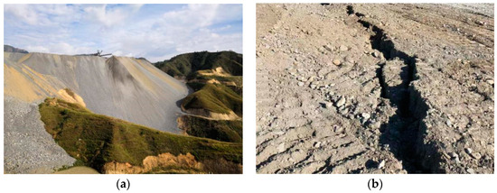
Figure 5.
(a) Belt dumping process; (b) front edge cracks of the platform due to natural settlement.
3. Introduction of the Calculation Method
With the development of computer technology, many numerical methods have been adapted, and each one has advantages and disadvantages. It is difficult to find a method that satisfies the requirements of both theoretical and practical applications. In the conventional LEM method, the Mohr–Coulomb failure criterion is generally used for soil, and the parameters are internal friction angle and cohesion. However, its applicability is limited because the most dangerous sliding surface of a rock slope is controlled by joints and fissures, and its strength cannot be determined only by the cohesion and internal friction angle of the material itself, and cannot reflect the dynamic process of the slope changing with time. The discrete element method corresponding to the particle flow methods does not need to define the constitutive relationship and corresponding parameters for the material in the calculation. These traditional mechanical properties and parameters are automatically obtained by the program. The parameters of the particle flow are mainly the contact stiffness between the particles, friction, bonding medium strength, etc. The SPH method needs to input terrain data, discrete slope particle information, and rock and soil parameters, and is calculated by an explicit method. The stress and strain calculation of MPM is based on the material constitutive model. The Drucker–Prager elastoplastic constitutive model (DP) is used for the muck material of our dump. The main parameters include internal friction angle, cohesion, Young’s module, and Poisson’s ratio because the tensile strength is ignored by the granular. Therefore, in this study, the SPH and MPM methods, two independent and interrelated methods, were used to calculate the dynamics of the movement of the waste and the speed, migration range, hazard area, and accumulated thickness of waste under different working conditions.
3.1. Introduction of the MPM Method
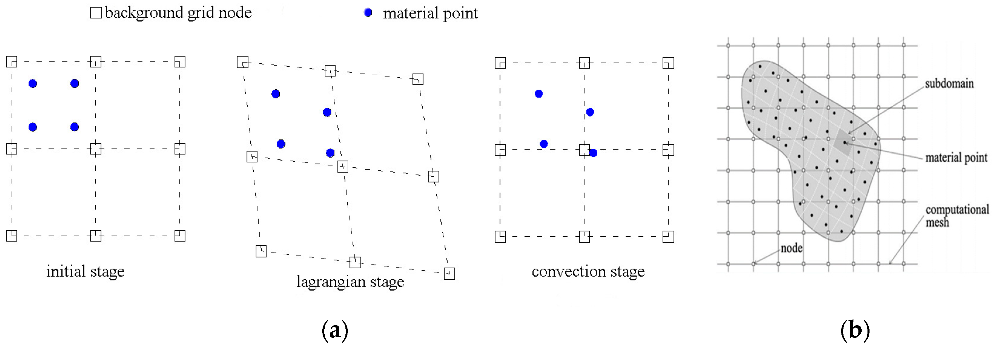
As a recently developed representative meshless particle method, the MPM discretizes a continuum research object into a series of particles. Each particle represents a part of the object within the corresponding range and contains all the material information of the corresponding area, including stress, strain, quality, and speed. At the same time, a background grid is established for solving the equation of motion in the calculation area, as shown in Figure 6a,b.
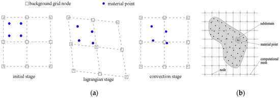
Figure 6.
(a) Material point method calculation process diagram; (b) material point discrete representation object.
The basic governing equations of the MPM are the mass conservation equation,
and the momentum conservation equation
where is the density at the current moment, represents the material speed, represents the Cauchy stress tensor, and represents the physical force. The mass of the particle does not change during calculations with the MPM, and thus the mass conservation equation is naturally satisfied in the calculation process. The calculation process is mainly used to solve the momentum conservation equation. Since the information about the object in the MPM is carried by the particle and the solution of the motion of the object is solved by the Euler background grid, the mass, momentum, stress, body force, and surface force of the particle at time t should be mapped to the background grid node. After the background grid node completes the calculation, the calculated motion parameters are mapped back to the particle, and the velocity and position of the particle are updated. The specific implementation steps are as follows:
- (1)
- The momentum and mass of each particle are mapped to the background grid node by an interpolation shape function to calculate the momentum and mass of the corresponding background grid node.
Among them, the subscripts I and represent the grid node variable and the material point variable, respectively, and n is the calculation step.
The operator ∑ represents the sum of all material points and is a shape function.
- (2)
- Essential boundary conditions are imposed on the nodes on the boundary. Let the nodes on the fixed boundary nodes make = 0.
- (3)
- The node velocity is calculated by the momentum of each grid node. The strain increment and the spin increment of each particle are calculated according to the velocity, and the stress of each particle is updated by the constitutive relationship:
Update the density of the particle:
- (4)
- Calculate the background grid node force internal force , node external force and total node force :
If the node is fixed in the i direction, then let = 0.
- (5)
- Integrating momentum equations on background grid nodes yields:
- (6)
- The position change and velocity change of the background grid node after calculation are mapped back to the corresponding particle before, and the displacement and velocity of the particle are updated:
- (7)
- To date, all the material information of the object has been updated and stored on the particle, the deformed mesh can be discarded, and the regular background calculation mesh can be redivided at the next time step, Figure 6b.
The MPM uses particles to discretize the material area and the background grid is used to calculate the spatial derivative and solve the momentum equation and prevent grid distortion and convection term processing, and has the advantages of the Lagrange and Euler algorithms. It is very suitable for simulations involving large deformation of materials and long-distance movement.
3.2. Introduction of the SPH Method
The smoothed particle hydrodynamics (SPH) method solves partial differential equations or integral equations through a series of interaction points carrying material information. It is a meshless, stable, and adaptive Lagrangian dynamics solution method and obtains accurate and stable numerical solutions. It has been widely used in the field of simulation calculations of disasters such as landslides and collapses.
Based on the Lagrangian description, the basic rules of mass conservation, momentum conservation, and energy conservation can be written as Navier–Stokes partial differential equations, as shown below:
where the superscript represents the coordinate direction, is the density, is the velocity, is the stress tensor, is the volume stress component, and is the time. The SPH form of the equation can be written as
In addition, the momentum equation in the form of the SPH method can be written as
where is the pressure of rock and soil, is the stress tensor, is the Kronecker symbol, is the viscosity coefficient of large deformation of rock and soil, is the yield stress, is the pure shear strain rate, and is the deviatoric strain rate tensor, The Greek letter superscripts and represent the coordinate direction. The pure shear strain rate and the deviatoric strain rate tensor are defined as
where is the volumetric strain rate and is the strain rate tensor, which is defined as
where , are the fluid velocities, and and are fluid coordinates.
The yield strength based on the Drucker–Prager yield criterion can be defined as
where is the friction coefficient of rock and soil, and is the cohesion.
4. Calculation Parameters and Terrain Acquisition
4.1. Terrain Acquisition and 3D Model Construction of the Dump
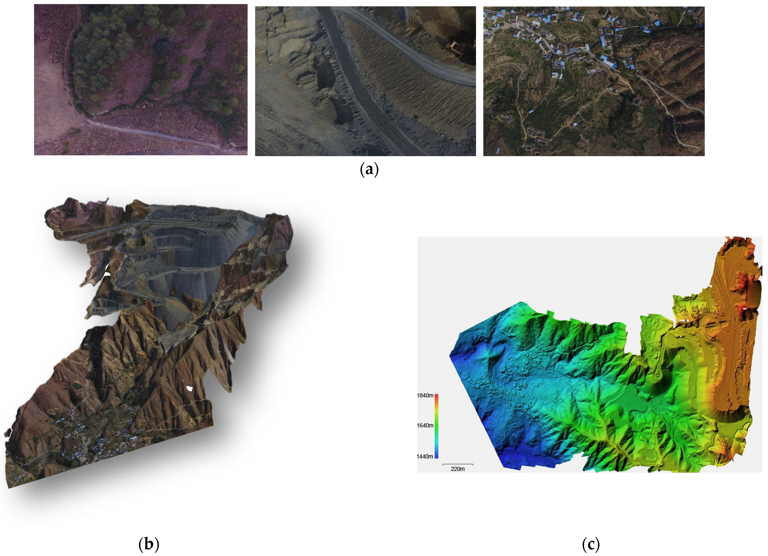
To obtain high-precision images of the terrain of the field area and extract the topography, a UAV was used to conduct orthophotographic imaging of the field area. Considering the computational power and accuracy of the computer, the final grid accuracy was set to 10 m. Agisoft photoScan 1.1.5 or Smart3D Context Capture 10.20 and other related software were used to stitch and proofread the photos, build DEM maps, point cloud maps, etc., and ArcGIS 10.6 was used for terrain processing, as shown in Figure 7a–c, which provides basic data for subsequent numerical calculations.
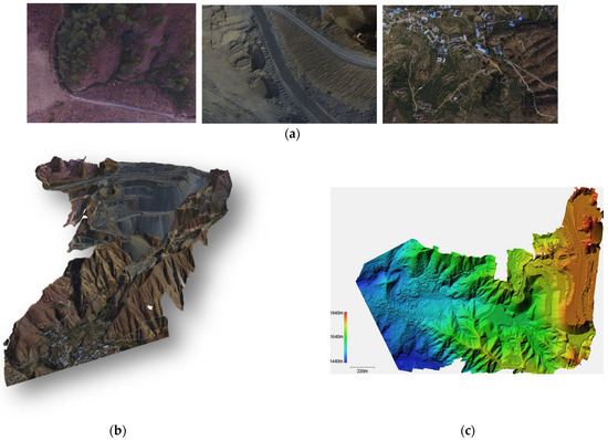
Figure 7.
(a) Unmanned aerial photography; (b) image of the dump; (c) orthographic DEM.
4.2. Calculation Parameters
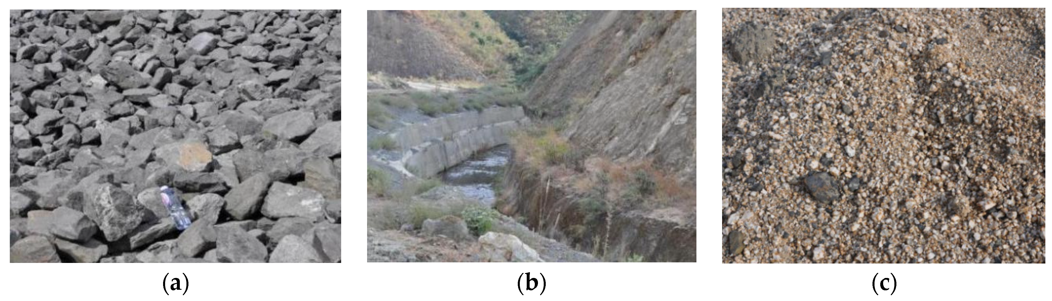
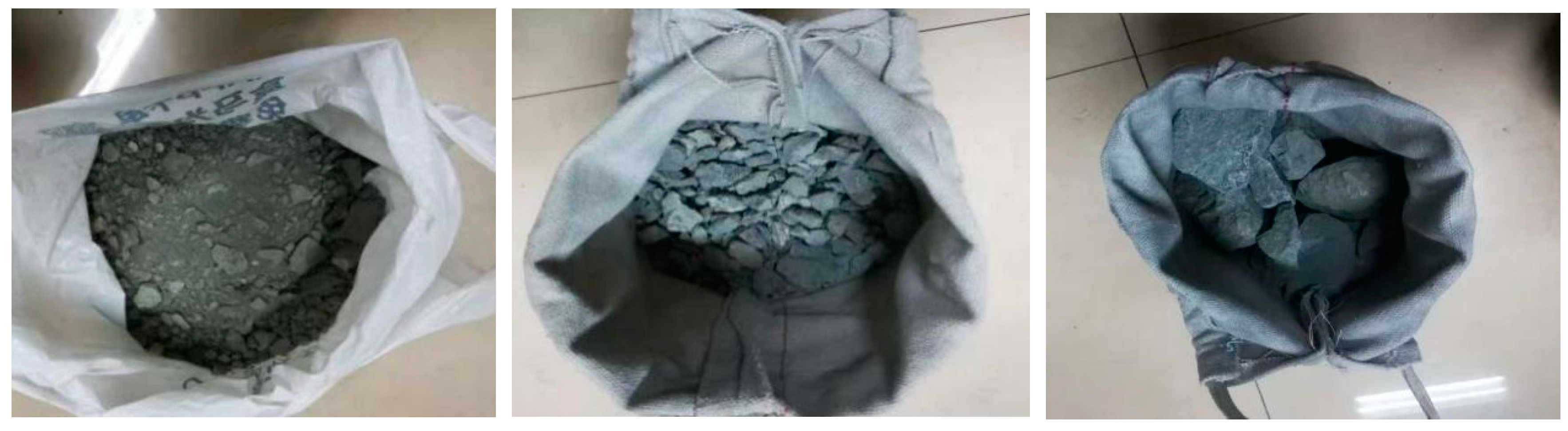
In order to ensure the accuracy of the numerical simulation results based on the actual terrain and obtain the calculation parameters and conventional physical and mechanical parameters required for numerical calculation, the cooperative test company collected the rock and soil samples in the field area through field investigation. There were three sample collection points. The first sample collection point was the outlet of the conveyor belt on the upper part of the waste, and the freshly stacked slag was collected; the second sample collection point was the lower part of the waste, and the slag slipped downward through the waste slope was collected. The third sample collection point was the outcrop of the cover layer around the waste, and the exposed cover layer was mainly weathered granite, as shown in Figure 8 and Figure 9.

Figure 8.
(a) Sampling sites at (a) the outlet; (b) the toe of the waste slope; and (c) the covering layer around the waste.
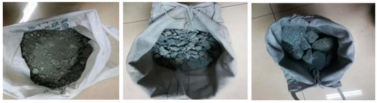
Figure 9.
Test samples (Wast from three sample collection points).
Through the physical and mechanical tests of indoor rock and soil, standard penetration test, N63.5 heavy dynamic penetration test, direct shear test, consolidated drainage shear test, (Table 1 and Table 2), and an on-site excavation of the waste soil in the dump site, screening was performed to determine the particle gradation of the waste soil. Through the dry particle flow experiment in the channel and consulting the relevant specification manual, and based on the experience, the friction coefficient of the rock and soil base was obtained. The calculation parameters are shown in Table 3 and Table 4.

Table 1.
Statistical table of standard penetration test results.
Table 2.
Statistics of heavy dynamic penetration test results (N63.5).
Table 3.
(a) Strength parameters of waste materials under different working conditions. (b) Strength parameters of waste materials under different working conditions.
Table 4.
Simulation material parameters of the dump.
The investigation and available data show that the climate in the area is dry, the rainfall is less, and the long-term evaporation is much stronger than the rainfall, and thus the rock and soil in the area are always in a relatively dry state. The research shows that this kind of rock and soil mass and slope are more prone to instability and failure under the action of short-term high-intensity rainfall. There have been no earthquakes above magnitude 7 in the field area and its vicinity, and there are large faults such as the Xigeda fault and the Anninghe fault zone near the field area. Under the action of occasional super-strong earthquakes, the discards are destroyed as a whole or locally due to the tensile shear of the seismic force. However, because the discards contain no viscous material and are strongly permeable to water, there is no excess pore pressure, superfluidity, and seismic liquefaction, and thus migration after destruction is limited. Under the action of super-heavy rainfall, if the drainage system in the field area cannot be drained quickly or fails as a whole, the hydrostatic pressure inside the dump increases rapidly, and the effective stress between the particles of the waste decreases rapidly, resulting in a decrease in the resistance of the waste to shear failure, rapid instability, and the development of superfluidity. Therefore, this study examined the migration of waste after instability and failure under two different working conditions, namely, a conventional state and a super-heavy rainfall, and provided the range of potential threats.
5. Dynamic Simulation
5.1. Dynamics Simulation Based on the MPM
5.1.1. Construction of the MPM
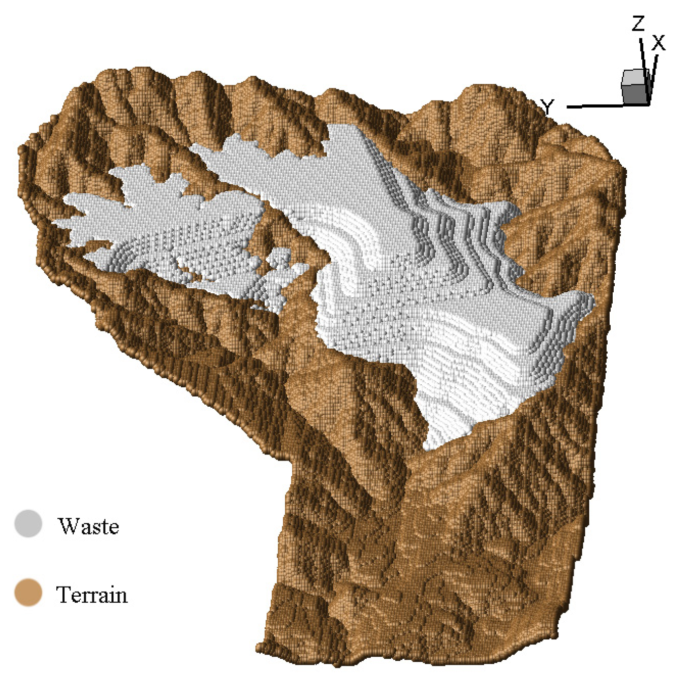
A three-dimensional real digital elevation model of the waste was constructed from the elevation data before and after the slag accumulation obtained by the field investigation, and then the numerical calculation model of the MPM is constructed. Considering the actual calculation efficiency and accuracy, a material point represents 10 m × 10 m × 10 m, as shown in Figure 10. Among them, the brown-yellow color represents the actual terrain on the bottom, with a total of 87,963 material points, and the gray-white color represents the waste, with a total of 113,176 material points. The bedrock of the bottom surface of the field area is granite, and the integrity is good. In the actual calculation, the granite bedrock surface was set as a rigid surface, and the friction coefficient between the granite bedrock and the waste was set to 0.3. The calculation results were obtained on the basis of satisfying the granite bedrock without damage. The dump is located in a high-intensity area. Two working conditions were considered in the calculations: ordinary working conditions and rainfall conditions. The strength parameters of the waste material determined by the indoor experiment are shown in Table 3.
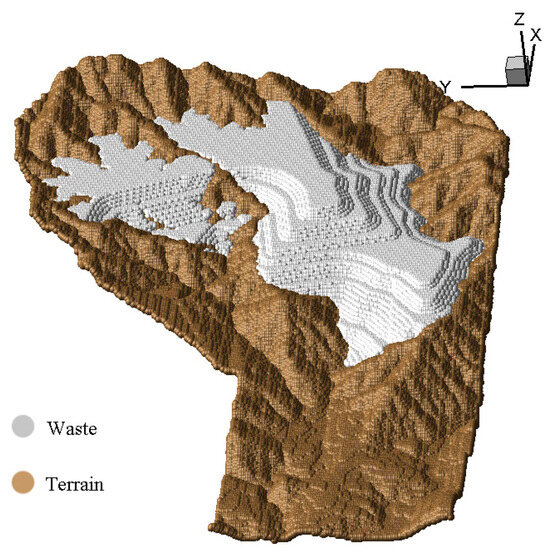
Figure 10.
MPM numerical calculation model based on the actual terrain.
In this simulation, the Drucker–Prager model and the parameter values in Table 3 were adopted for the rock and soil mass, and the MPM numerical calculation model based on the actual terrain was constructed.
5.1.2. Numerical Results and Analysis
- 1.
- Calculation results and analysis under normal conditions
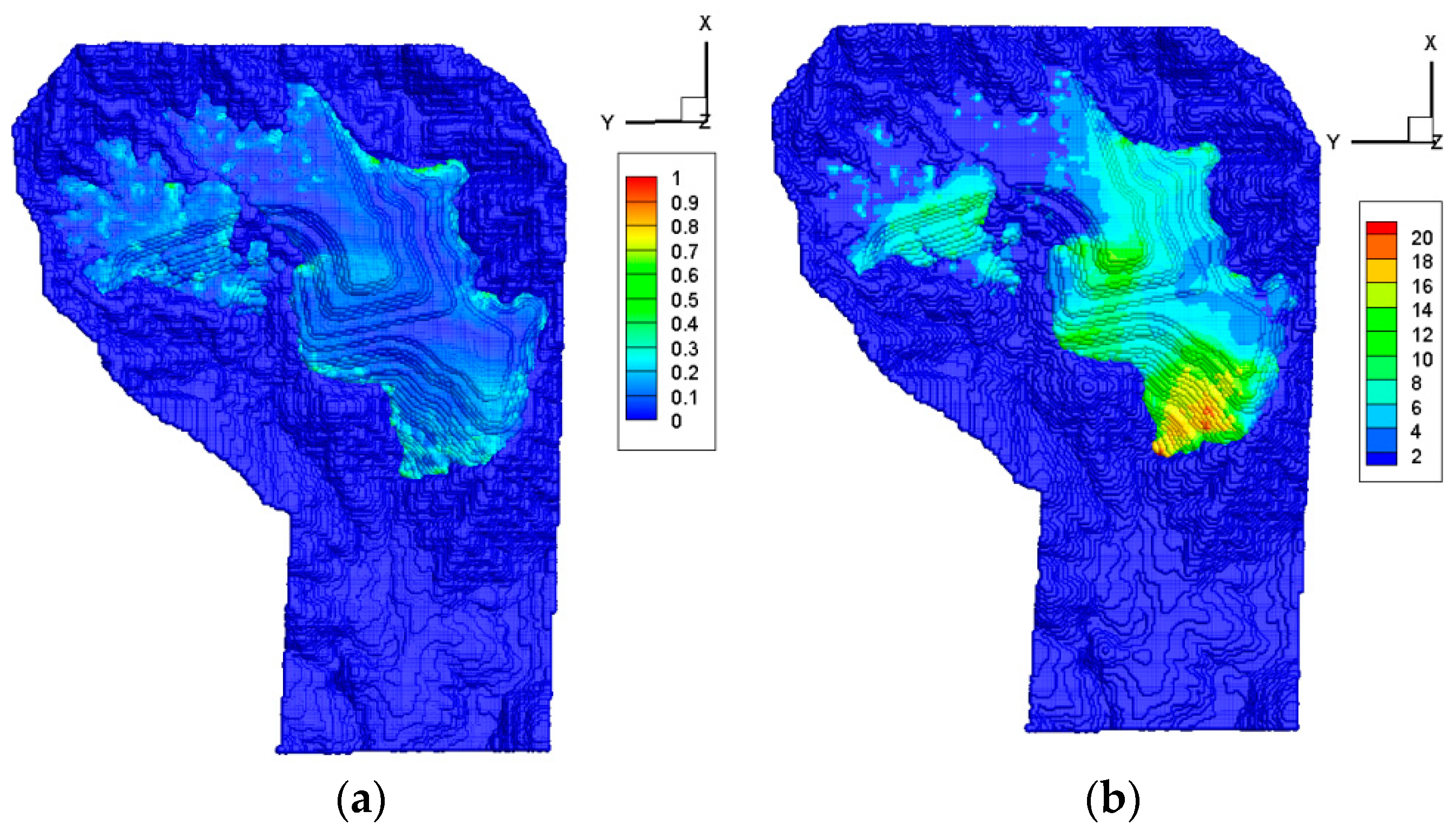
Under this condition, the waste was stable as a whole, and there was no obvious large-scale failure behavior. The equivalent plastic strain value after 200 s is shown on the left side of Figure 11. The equivalent plastic strain value of the waste was small, less than 1, and the larger value was mainly concentrated at the slope angle of the waste. The right side of Figure 11 shows the total (spatial) displacement of the waste after 200 s of calculation. The maximum displacement (oblique distance) was 21.75 m, which mainly appeared on the slope above the dam in front of the slag yard. Overall, this is reflected in the destruction of the slope surface.

Figure 11.
Equivalent plastic strain (a) and displacement (m) (b) of the waste field under ordinary working conditions.
- 2.
- Calculation results and analysis under rainfall conditions
Under this working condition, the waste mainly underwent instability failure above the front side of the dam body, and the rear side was relatively stable. For example, the left side of Figure 11 shows the equivalent plastic strain value after calculating for 1200 s. The maximum equivalent plastic strain of the waste was concentrated on the leading edge of the movement, which is 3.7. Among them, the larger value was concentrated at the position of the slope angle. Compared with the ordinary working conditions, the overall equivalent plastic strain of the slag field increased obviously and continued to increase with increasing distance moved. The right side of Figure 12 shows the total (spatial) displacement of the waste after 1200 s under this working condition. The maximum (spatial) displacement was 385.48 m, and the waste almost rushed out of the ditch.

Figure 12.
Equivalent plastic strain (a) and displacement (m) (b) of the dump under rainfall conditions.
It should be emphasized that the maximum spatial displacement given by the calculation was calculated based on the three-dimensional spatial position of the damaged part before and after movement, and the actual horizontal displacement was less than this value. The calculation correction shows that the maximum horizontal displacement under rainfall conditions was 352.4 m, but it was 322 m from the toe of the waste dump slope.
5.2. SPH-Based Dynamic Simulation
5.2.1. Construction of the SPH Model
According to experimental studies of the large deformation of soil at home and abroad, when soil undergoes a large deformation, X, there is a nonlinear relationship between the shear strain rate and shear stress, which can be described by a non-Newtonian fluid model. According to the terrain data before and after the landfill, the model was established. The particle spacing was 10.0 m. According to the initial terrain data, the thickness of the accumulation area was obtained, and the original terrain of the accumulation area was reconstructed, as shown in Figure 13a. Finally, the physical model for calculations was constructed.
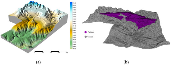
Figure 13.
(a) The terrain after filling of the dump; (b) three-dimensional physical model of the dump (schematic).
To prevent the particle penetration problem, two layers of particles were laid on the boundary, which is suitable where particles are sparse. The final number of boundary particles was 158,750, and the number of particles in the source area was 115,494. The physical model of the source region is shown in Figure 13b.
The dump is located in a high-intensity area. In the calculation process, ordinary conditions and heavy rainfall conditions were considered. The parameters required for calculation are shown in Table 4.
5.2.2. Numerical Calculation Results and Analysis
- 1.
- Analysis of calculation results under ordinary working conditions
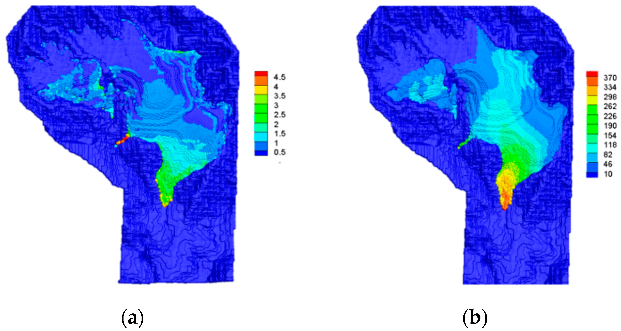
The dynamic evolution process of dump waste under ordinary working conditions is shown in Figure 14. The waste of the dump is in a stable state as a whole. The maximum displacement occurred on the surface of the slope on the upper left side of the larger waste, and the maximum spatial displacement was approximately 20 m. There was no obvious displacement inside the slope, and the slope did not collapse in a large range. The front edge of the waste did not exceed the initial accumulation range.
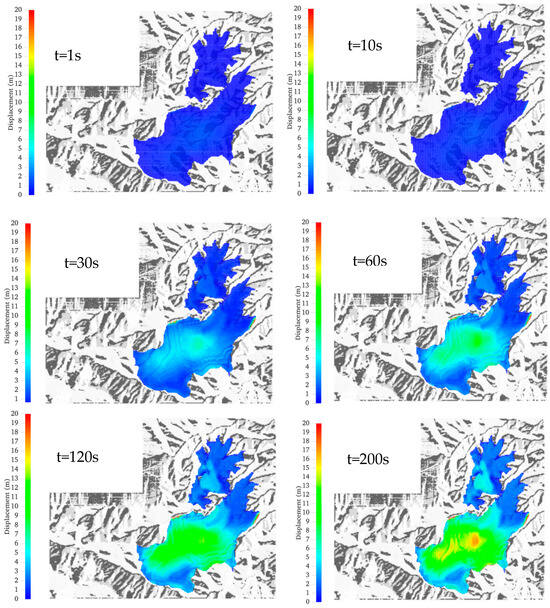
Figure 14.
The evolution of the spatial displacement of dump waste (under ordinary working conditions).
- 2.
- Calculation results and analysis under heavy rainfall conditions
Under the condition of heavy rainfall, the dynamic evolution of dump waste is shown in Figure 15. According to the calculation results, there were obvious instabilities and rapid sliding behaviors in the waste dump. The maximum displacement occurred on the upper left slope surface of the larger waste dump, and the maximum spatial displacement was 460 m. The slope collapsed over a large range, and the front edge of the waste dump rushed out of the valley. It should be emphasized that the maximum horizontal displacement of the waste was approximately 394 m, and the horizontal distance from the slope toe of the dump was approximately 370 m.
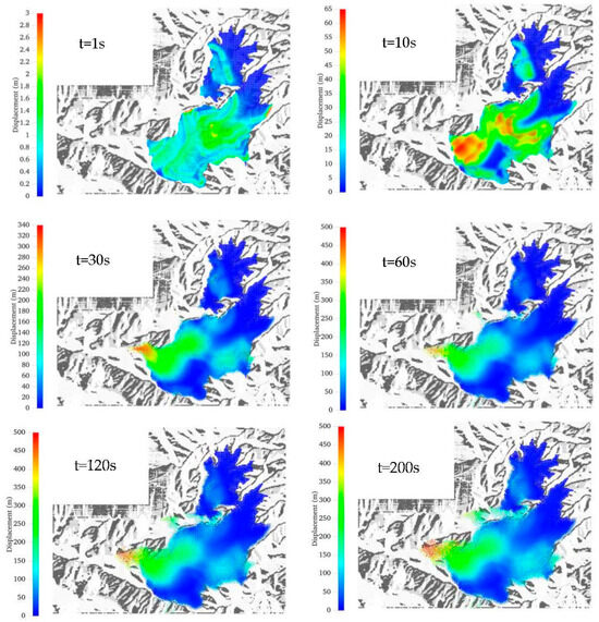
Figure 15.
The evolution of the spatial displacement of dump waste (under heavy rainfall conditions).
Figure 16 is the plane displacement of the waste, which is the comparison between the final dangerous area and the original spatial position of the waste. From the diagram, it can be seen that the maximum horizontal displacement of the waste was about 394 m, and the horizontal distance from the foot of the dump slope was 370 m.
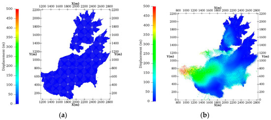
Figure 16.
The plane displacement: (a) the original spatial position and (b) the final dangerous area.
6. Discussion
The numerical simulation method shows potential that cannot be ignored in the risk assessment of abandoned slag slopes.
The research on the stability evaluation of waste slag slopes is mainly studied from both qualitative and quantitative aspects. The qualitative methods mainly include the natural history analysis method and the engineering geological analogy method. The results are subjective and empirical. The quantitative methods include the physical model test method, field monitoring, and numerical simulation method. Among them, the physical model test method is limited by various factors, and it is difficult to make the physical model and the real model fully meet the similarity, which has great limitations in use. On-site monitoring is required to clarify the main sliding direction and landslide mode of the deformation zone through displacement monitoring data and to analyze the changes in the seepage field of the dump from the inside to understand the internal factors that cause the landslide of the dump. However, due to the limited operability of the monitoring range, the cost is high, and the data accuracy is low and limited.
The numerical simulation method can effectively avoid the size effect of the model and simulate complex geological problems. It is more practical than the traditional laboratory or expensive, time-consuming, and even dangerous test methods. The influence of topography on landslides is very complex. The numerical simulation method has the advantage of considering the influence of actual terrain.
By simulating the instability process of the spoil slope, the 3D-MPM and 3D-SPH methods were compared.
Traditional Euler grid algorithms, such as the finite element method (FEM), are limited by the grid distortion and are more suitable for solving small deformation problems. The finite difference and finite volume methods based on depth averaging can better reflect the control effect of the actual terrain and have higher computational efficiency. However, these methods are essentially two-dimensional methods, which mainly focus on the base friction and need to preset the sliding surface, which is not conducive to the solution of the instability process of the spoil slope.
In this context, some meshless numerical methods, such as the smoothed particle hydrodynamics method and material point method, are applied to the calculation of the slope dynamic process. In this study, these two methods were used to reflect the similar instability movement process of the spoil slope. From the point of view of the instability process and the final movement distance, the results are similar. Under ordinary working conditions (static and dry conditions), the dump is in a stable state, and only local shallow surface damage or shallow surface damage occurs at some steps. Under the condition of heavy rainfall, it is assumed that the waste is close to saturation, the fluidity is strong, the movement is triggered due to excessive water content, and a large-scale instability failure occurs. The disadvantage is that there is no earthquake condition involved in this paper. Although there has been no earthquake above 7 magnitude in the project area and its vicinity, the probability of a super strong earthquake is very low, but this possibility cannot be completely ruled out. Two cases can be considered, only seismic load, and seismic load and extreme rainfall conditions. This is a problem that needs to be further discussed in the future. Through the two methods of MPM and SPH, the maximum horizontal displacements of the waste were 352.4 m and 394 m, respectively. The two methods verified each other and increased the reliability of the simulation.
7. Conclusions
With the rapid development of computer technology, various numerical methods provide many new directions and possibilities for the study of geological disasters. Each method has its own adaptability, advantages, and disadvantages. It is difficult to find a method that satisfies both theory and practical application. Taking the Panzhihua dump as an example, the authors analyzed the landform, stratum lithology, geological structure, and engineering geological conditions of the study area through field investigation. SPH and MPM, two independent and interrelated methods, were used to calculate the dynamics of the movement of the waste under ordinary conditions and heavy rainfall conditions. The calculation results based on MPM show that under natural conditions, the waste of the dump is stable as a whole, and the local shallow surface is slightly damaged; under the action of extreme rainfall, the effective stress between the particles inside the waste is reduced, and the overall stability is reduced and eventually destabilized. After the instability, the debris moves forward rapidly, and the maximum spatial displacement reached 385.48 m, almost rushing out of the gully. At this time, the maximum horizontal displacement was 352.4 m. The results based on the SPH method showed that under natural conditions, the waste in the dump was in a stable state, and shallow damage occurred at some steps. Under extreme rainfall conditions, large-scale instability and failure of the waste occurred. At this time, the maximum horizontal displacement was about 394 m, and the horizontal distance from the slope toe of the dump was about 370 m. Based on the comprehensive analysis, the maximum value of 370 m was taken as the basic value of the potential threat distance (corresponding to the maximum spatial displacement of 460 m and the maximum horizontal distance of 394 m) from the design of the leading edge slope toe of the waste dump, and the safety reserve was enlarged appropriately. Finally, 400 m was determined as the final range of the potential threat of the dump. The research results are conducive to the risk assessment of the spoil slope.
The multi-method analysis has a positive role in promoting the research on the prediction of the disaster range of the dump and provides a reference for similar disaster research.
Author Contributions
Conceptualization, D.L. and C.G.; methodology, D.L. and C.G.; formal analysis and investigation, X.S. and J.W.; writing—original draft preparation, D.L. and J.W.; writing—review and editing, C.G.; funding acquisition, C.G., D.L. and X.S. All authors have read and agreed to the published version of the manuscript.
Funding
This research is funded by the National Key Research and Development Program of China (No. 2023YFB2604005), the Scientific research project of Chongqing Planning and Natural Resources Bureau (No. KJ-2023046), the Key Research and Development Project of Henan Province (Science and Technology Research Project) (No. 232102320028), Research on the teaching reform of vocational education in Henan Province (No. 05853), The National Nature Science Foundation of China (No. 41472325).
Institutional Review Board Statement
Not applicable.
Informed Consent Statement
Not applicable.
Data Availability Statement
The raw data supporting the conclusions of this article will be made available by the authors on request.
Acknowledgments
The author would like to thank Siming He and Xinpo Li from the institute of Mountain Hazards and Environment for their valuable discussion in this paper.
Conflicts of Interest
The authors declare that they have no known competing financial interests or personal relationships that could have appeared to influence the work reported in this paper.
References
- Rajak, T.K.; Yadu, L.; Chouksey, S.K.; Dewangan, P.K. Stability analysis of mine overburden dump stabilized with fly ash. Int. J. Geotech. Eng. 2021, 15, 587–597. [Google Scholar] [CrossRef]
- Gupta, G.; Sanjay, K.; Sharma Singh, G.S.P.; Kishore, N. Numerical Modelling-Based Stability Analysis of Waste DumpSlope Structures in Open-Pit Mines—A Review. J. Inst. Eng. 2021, 102, 589–601. [Google Scholar] [CrossRef]
- Omraci, K.; Merrien-Soukatchoff, V.; Tisot, J.P.; Piguet, J.P.; Le Nickel, S.L.N. Stability analysis of lateritic waste deposits. Eng. Geol. 2003, 68, 189–199. [Google Scholar] [CrossRef]
- Rai, R.; Khandelwal, M.; Jaiswal, A. Application of geogrids in waste dump stability: A numerical modeling approach. Environ. Earth Sci. 2012, 66, 1459–1465. [Google Scholar] [CrossRef]
- Quezada, J.C.; Villavicencio, G.E. Discrete modeling of waste rock dumps stability under seismic loading. EPJ Web Conf. 2021, 249, 11013. [Google Scholar]
- Zhang, W.; Zheng, H.; Jiang, F.; Wang, Z.; Gao, Y. Stability analysis of soil slope based on a water-soil-coupled and parallelized Smoothed Particle Hydrodynamics model. Comput. Geotech. 2019, 108, 212–225. [Google Scholar] [CrossRef]
- Sulsky, D.; Chen, Z.; Schreyer, H.L. A particle method for history-dependent materials. Comput. Methods Appl. Mech. Eng. 1994, 118, 179–196. [Google Scholar] [CrossRef]
- Bhandari, T.; Hamad, F.; Moormann, C.; Sharma, K.G.; Westrich, B. Numerical modelling of seismic slope failure using MPM. Comput. Geotech. 2016, 75, 126–134. [Google Scholar] [CrossRef]
- Conte, E.; Pugliese, L.; Troncone, A. Post-failure stage simulation of a landslide using the material point method. Eng. Geol. 2019, 253, 149–159. [Google Scholar] [CrossRef]
- Conte, E.; Pugliese, L.; Troncone, A. Post-failure analysis of the Maierato landslide using the material point method. Eng. Geol. 2020, 277, 105788. [Google Scholar] [CrossRef]
- Li, X.; Tang, X.; Zhao, S.; Yan, Q.; Wu, Y. MPM evaluation of the dynamic runout process of the giant Daguangbao landslide. Landslides 2021, 18, 1509–1518. [Google Scholar] [CrossRef]
- Li, X.; Wu, Y.; He, S.; Su, L. Application of the material point method to simulate the post-failure runout processes of the Wangjiayan landslide. Eng. Geol. 2016, 212, 1–9. [Google Scholar] [CrossRef]
- Li, X.; Yan, Q.; Zhao, S.; Luo, Y.; Wu, Y.; Wang, D. Investigation of influence of baffles on landslide debris mobility by 3D material point method. Landslides 2020, 17, 1129–1143. [Google Scholar] [CrossRef]
- Gingold, R.A.; Monaghan, J.J. Smoothed particle hydrodynamics: Theory and application to non-spherical stars. Mon. Not. R. Astron. Soc. 1977, 181, 375–389. [Google Scholar] [CrossRef]
- Aaron, J.; Hungr, O. Dynamic simulation of the motion of partially-coherent landslides. Eng. Geol. 2016, 205, 1–11. [Google Scholar] [CrossRef]
- Cola, S.; Calabro, N.; Pastor, M. Prediction of the flow-like movements of Tessina landslide by SPH model. In Proceedings of the 10th International Symposium on Landslides and Engineered Slopes, Xi’an, China, 30 June–4 July 2008. [Google Scholar] [CrossRef]
- Haddad, B.; Pastor, M.; Palacios, D.; Munoz-Salinas, E.A. SPH depth integrated model for Popocatepetl 2001 lahar (Mexico): Sensitivity analysis and runout simulation. Eng. Geol. 2010, 114, 312–329. [Google Scholar] [CrossRef]
- Pastor, M.; Blanc, T.; Pastor, M.J. A depth-integrated viscoplastic model for dilatant saturated cohesive-frictional fluidized mixtures: Application to fast catastrophic landslides. J. Non-Newton. Fluid Mech. 2009, 158, 142–153. [Google Scholar] [CrossRef]
- Pastor, M.; Blanc, T.; Haddad, B.; Petrone, S.; Sanchez Morles, M.; Drempetic, V.; Issler, D.; Crosta, G.B.; Cascini, L.; Sorbino, G.; et al. Application of a SPH depth-integrated model to landslide run-out analysis. Landslides 2014, 11, 793–812. [Google Scholar] [CrossRef]
- Bui, H.H.; Fukagawa, R.; Sako, K.; Ohno, S. Lagrangian meshfree particles method (SPH) for large deformation and failure flows of geomaterial using elastic-plastic soil constitutive model. Int. J. Numer. Anal. Methods Geomech. 2008, 32, 1537–1570. [Google Scholar] [CrossRef]
- Bui, H.H.; Fukagawa, R.; Sako, K.; Wells, J.C. Slope stability analysis and discontinuous slope failure simulation by elasto-plastic smoothed particle hydrodynamics (SPH). Geotechnique 2011, 61, 565–574. [Google Scholar] [CrossRef]


Disclaimer/Publisher’s Note: The statements, opinions and data contained in all publications are solely those of the individual author(s) and contributor(s) and not of MDPI and/or the editor(s). MDPI and/or the editor(s) disclaim responsibility for any injury to people or property resulting from any ideas, methods, instructions or products referred to in the content. |
© 2024 by the authors. Licensee MDPI, Basel, Switzerland. This article is an open access article distributed under the terms and conditions of the Creative Commons Attribution (CC BY) license (https://creativecommons.org/licenses/by/4.0/).