Abstract
The permeability coefficient of landslide mass, a key parameter in the study of reservoir landslides, is commonly obtained through in situ and laboratory tests; however, the tests are costly and subject to high variability, leading to potential biases. In this paper, a new method was proposed to inversely estimate the permeability coefficient of landslide layers using monitoring data of groundwater level (GWL). First, the landslide transient seepage simulation was conducted to generate sample data for permeability coefficients and GWL during a reservoir operation cycle. Second, using GWL data as input and permeability coefficient data as output, the least-square support vector machine (LSSVM) was trained with two optimization algorithms, the particle swarm optimization (PSO) algorithm and the whale optimization algorithm (WOA), to construct the nonlinear mapping relationship between simulated GWL and permeability coefficients. Third, the accurate permeability coefficients for landslide seepage simulation were inverted or predicted based on the monitored GWL. Finally, using the inverted permeability coefficients for landslide seepage simulation, we compared simulation results with actual monitored GWL and achieved good consistency. In addition, this paper compared the inversion effects of three different algorithms: the standard LSSVM, PSO-LSSVM, and WOA-LSSVM. This study showed that these three algorithms had good nonlinear fitting effects in studying landslide seepage fields. Among them, using the inversion values from PSO-LSSVM for landslide seepage simulation resulted in the smallest relative error compared to actual monitoring data. Within a single reservoir operation cycle, the simulated water level changes were also largely consistent with the monitored water level changes. The results could provide a reference to determine landslide permeability coefficients and seepage.
1. Introduction
As the global demand for clean energy continues to rise, the construction of hydroelectric projects is thriving. The construction and operation of reservoirs significantly alter the original slope morphology and hydraulic conditions, becoming primary factors in the occurrence of geological disasters within reservoir areas. Among these, reservoir landslides are the most common type of geological disaster caused by human activities in these areas. For instance, in China’s Three Gorges Reservoir area, over 5000 landslides or potential landslides have been identified.
To accurately predict and effectively prevent reservoir landslides, studying their deformation and evolution mechanisms is essential. Reservoir landslides exhibit multi-field information evolution characteristics dominated by periodic changes in seepage fields. The seepage field of landslides is crucial for studying the mechanism of reservoir landslide formation and deformation failure modes [1,2,3,4].
Currently, the main methods for studying seepage fields in reservoir landslides include theoretical analysis, field monitoring, and numerical simulation. Among these, field monitoring of the GWL in landslides shows the dynamic response of GWL in a landslide mass to reservoir water levels (RWL), which helps analyze landslide seepage fields. However, this monitoring data alone cannot fully capture the periodic variations in the reservoir landslide seepage field and its impact on the landslide stability. Therefore, further research using theoretical analysis or numerical simulation is necessary. For both theoretical analysis and numerical simulation, determining the permeability coefficient of a landslide mass is essential. The difficulty in parameter determination has always been a bottleneck in theoretical analysis and numerical simulation in geotechnical mechanics.
Traditional testing methods such as pumping tests [5,6] are simple and convenient. However, because the test locations are discrete and the parameters have nonuniformity, the results often fail to reflect the comprehensive seepage parameters of rock and soil masses [7]. Due to practical constraints, it is also difficult to conduct relevant tests on deep-seated rock masses in landslides. In addition to experimental methods, permeability coefficients of aquifers can be determined using analytical methods [8], but this route is limited to simple seepage field conditions or simplified assumptions. The relationship between seepage parameters of landslide masses and GWL is complex and nonlinear, so it is difficult to directly express using formulas.
With the development of monitoring technology, using monitoring data to invert the parameters of landslides has become an important approach over the past decades. The displacement back-analysis method is widely used in the parameter inversion of landslide masses and tunnel surrounding rock. Deng and Lee [9] developed a novel method for displacement back-analysis of rock slopes, using the Three Gorges Project site as a case study. With the development of machine learning, an increasing number of algorithms are being applied to data analysis in engineering fields, addressing many complex engineering problems. Kazemi et al. [10,11] employed 20 machine learning methods to assess the seismic response and performance of reinforced concrete buildings, and to analyze the seismic risk assessment of reinforced concrete structures. In recent years, combined with machine learning, the displacement back-analysis method has further developed. For example, scholars have used the neural network–genetic algorithm combination [12], artificial neural network optimization methods [13], and improved support vector machine methods [14,15,16] to conduct displacement back-analysis on the slope masses or tunnel surrounding rock, thereby determining the mechanical parameters of rock and soil materials.
With the increasing construction of reservoirs, the study of seepage fields in reservoir dams and slopes remains a hot topic in geotechnical engineering. Many advances have been made in seepage back-analysis research, especially regarding the inversion of permeability coefficients of dam bodies or dam foundations [17,18,19,20,21,22]. Some scholars also used machine learning methods to predict or inversely estimate the permeability coefficients of slope masses [23,24]. Yue et al. [25] conducted an inversion study of reservoir colluvial landslide permeability coefficient by combining physical models and data-driven models. Wang et al. [26] proposed an evolutionary neural network inversion method to invert saturated permeability coefficient from the monitoring data. Li et al. [27] established a model integrating the relevance vector machine and cuckoo search to accurately determine the permeability coefficients of strata. However, most existing studies use steady-state analysis to estimate seepage parameters. For reservoir bank slopes, where GWL fluctuate with reservoir operations, steady-state analysis fails to capture the actual seepage parameters. Therefore, transient groundwater flow analysis should be used to invert the permeability coefficients.
In the vast array of machine learning algorithms, support vector machine (SVM) is a regression method praised for its strong generalization and precise prediction. Compared to many neural networks, SVM is less likely to overfit with small training sets, thus having an advantage in various scenarios. Furthermore, LSSVM extends SVM using a least-square approach to formulate the objective function, leading to more efficient solving processes and superior generalization capabilities. Therefore, LSSVM was selected as the primary machine learning approach in this paper for inversion analysis.
This paper aims to obtain permeability coefficients of landslide mass suitable for transient analysis, with computed results consistent with monitoring data. To achieve this objective, two tasks were set: first, to construct training datasets for landslide permeability coefficients inversion based on finite element transient analysis; second, to compare the training effectiveness and inversion performance of LSSVM and its optimization algorithms to accurately determine permeability coefficients. The method proposed by this paper will provide new insights and reference to comprehensively determine the permeability coefficients of reservoir landslide.
2. Basic Method Principles
Due to the critical importance of LSSVM parameters on training outcomes, parameter optimization is necessary. Swarm intelligence algorithms are inspired by the collective behavior of natural groups and are used to solve complex optimization problems. Two swarm intelligence algorithms, PSO and WOA, are introduced in this study specifically to optimize the parameters of LSSVM. The basic principles of these three methods will be briefly introduced below.
2.1. Least-Square Support Vector Machine
LSSVM is a variant of support vector machine that has unique advantages in handling small samples and nonlinear problems [28,29]. SVM solves a quadratic programming problem with inequality constraints. LSSVM simplifies the problem by replacing the inequality constraints with equality constraints and changing the quadratic programming task into a linear one to reduce the complexity and significantly accelerate the solving process.
Suppose that the training set consists of (xi, yi), where i = 1, 2…, n. Here, xi ∈ Rm is the m-dimensional input vector of the system, and yi ∈ Rn is the corresponding output value. If the problem is nonlinear, the input vectors can be mapped to a high-dimensional space using a nonlinear mapping, which transforms the problem into a linear-like problem.
The minimization function for the optimization problem of the LSSVM is:
where w is the weight vector; C is the penalty factor, also known as the regularization constant. The constraints are as follows:
For the problem of LSSVM, according to Equations (1) and (2), the Lagrange solving equation is defined as follows:
where ai is the Lagrange multiplier.
The optimal values of parameters a and b can be obtained through Karush–Kuhn–Tucker (KKT) conditions.
From Equation (4), we obtain:
By eliminating w and from Equation (6), we transform the optimization problem into solving the following equation:
In the equation, .
Here, Ω is a matrix, and . Its inner product can be equivalently replaced by a kernel function in the original input space. Therefore, transform is not required to handle nonlinear problems. The inner product calculation directly adopts the kernel function, which is denoted as . After obtaining the values of parameters a and b, we can derive the regression model of the LSSVM:
Kernel function K (x, xi) is any symmetric function that must satisfy Mercer condition. Commonly used kernel functions include linear functions, radial basis functions (RBF), and polynomial functions. The LSSVM introduced in this paper uses the RBF kernel [30]. Parameter σ2 of the RBF kernel and penalty factor C in the expression of the LSSVM significantly affect the operation results of the LSSVM. Therefore, the selection of these two parameters determines the classification accuracy and fitting quality. Kernel parameter σ2 reflects the distribution characteristics of the training sample dataset, whereas penalty factor C adjusts the balance between the confidence range of LSSVM and the empirical risk. Therefore, finding the optimal parameters will improve the performance of LSSVM.
2.2. Particle Swarm Optimization
The PSO algorithm is an iterative optimization tool, and has advantages such as global optimization and a fast convergence speed [31]. In PSO, the solution to the problem is considered particles in the search space. Each particle represents a potential solution, and its fitness value is determined by an objective function (e.g., the mean square error between permeability coefficient sample values and predicted values, as shown in Equation (9)). The velocity of a particle determines its direction and distance of movement. The particle positions are dynamically adjusted based on the movement experience of the particle and that of other particles to achieve optimization in the feasible space.
In the equations, and are the permeability coefficient sample value and predicted value for the ith monitoring point and jth sample, respectively; n is the number of monitoring points; m is the number of samples.
PSO first generates a set of initial particles and assigns random values to the initial positions and velocities of the particles. By computing the fitness value of the particles, individual and global best positions are determined. Then, an iterative approach is used to seek the optimal solution. During the iteration process, the positions and velocities of particles are updated according to Equations (10) and (11), which involve tracking both individual and global best values. The individual best value is the best solution found by each particle in each search and denoted as the individual best . The global best value is the best solution found by all particles in the swarm in each search and denoted as the global best until convergence is achieved or the maximum iteration steps are reached.
where ω is the inertia weight; d = 1,2,…,D, D denotes the dimensions of the search space; i = 1,2,…, N, N represents the particles in the swarm; t is the current iteration number; is the velocity of the ith particle; and are the acceleration coefficients with values of (0,2); and are random numbers between (0,1); and are the current and updated velocities of the ith particle, respectively; and are the current and updated positions of the ith particle, respectively.
2.3. The Whale Optimization Algorithm
The WOA is a newly proposed swarm intelligence optimization algorithm in recent years with few parameters, fast convergence speed, and easy implementation [32]. The WOA simulates the hunting behavior of whales and introduces the bubble-net feeding strategy, which enables it to optimize specific problems. The WOA divides this hunting process into three stages as follows.
- Encircling prey: the WOA assumes the best individual in the current population as the prey. Other whale individuals in the population update their positions to approach the best individual. The mathematical model for this stage is:where X(t) is the position vector of the whale individual; t is the current iteration number; Xp(t) is the position vector of the prey; A and B are coefficient vectors and satisfy:r1 and r2 are random vectors in the interval [0, 1]; a is a regulating factor that linearly decreases from 2 to 0 with the increase in number of iterations, i.e.,:tmax is the maximum number of iterations. By decreasing the value of vector a, the population gradually approaches the prey, performing encircling prey.
- Spiral update: The mathematical model to update the positions in the spiral update is:where D′ = |Xp(t) − X(t)| is the distance between the current individual and the prey; b is a constant; l is a random number in the interval [−1, 1].
During the hunting process, whales simultaneously encircle the prey and ascend towards it along a spiral path. Therefore, in the optimization process, when |A| < 1, the population performs encircling prey or spiral update. Encircling prey and spiral update have equal probabilities of being selected, as shown in Equation (16):
where p is an arbitrary number in the range of [0, 1].
- 3.
- Random search: In addition to narrowing the encirclement during the spiral ascent, whales can randomly roam and search for prey during the hunting process. When r|A| ≥ 1, whales randomly search for prey based on their positions. The mathematical model for this process is:
2.4. Inverse Process of Landslide Seepage
Using the standard LSSVM, PSO-LSSVM and WOA-LSSVM to find the optimal parameters for LSSVM learning involves minimizing the difference between predicted permeability and sample permeability as the fitness function (Equation (9)) and calculating the optimal kernel function parameters to optimize the training effect for the support vector machine model. The specific steps of the inversion process are as follows. The flowchart is shown in Figure 1.
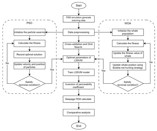
Figure 1.
Flowchart of landslide seepage inverse process.
- Define the permeability coefficient range for the landslide mass to be inverted and use a uniform design to establish the sample calculation scheme.
- Establish a finite element model and calculate the transient seepage over one reservoir operation cycle. The calculated GWL data were used as input, and the corresponding permeability coefficients were used as output ki to form learning samples.
- Train the LSSVM model: determine the optimal parameters (, ) of the standard LSSVM model using cross-validation and grid search. For LSSVM models optimized by swarm intelligence, obtain the optimal parameter values via iterative optimization using both the PSO algorithm and the WOA. Specifically, taking PSO as an example, the steps are as follows.
- (a)
- Initialize the swarm intelligence algorithm, including the swarm size, weight factors for each particle, number of iterations, randomly generated particle swarm vectors, and corresponding C and σ2 values for each particle vector. Use the learning sample set as training and validation samples. Set the individual extremes of each particle to the current position, input them into LSSVM for training, and obtain the corresponding predicted permeability coefficients.
- (b)
- Calculate the average relative error between corresponding predicted values and actual values for each particle and use it as the fitness value for each particle. Then, iterate the calculation, update the velocity and position parameters of each particle, and memorize the best fitness values that correspond to individuals and the global optimum. When the initially set maximum number of iterations is reached, terminate the calculation and remember the best (C, σ2).
- Substitute the optimal parameters (C, σ2) obtained from step 3b into the LSSVM model to establish the nonlinear mapping relationship between the permeability of the landslide mass and the GWL.
- Use GWL monitoring data from landslides to predict the permeability coefficients of the landslide mass. Incorporate these coefficients into the transient analysis simulation to invert the landslide seepage field.
3. Engineering Case Study
3.1. Engineering Overview
Majiagou landslide is located in Guizhou Town, Zigui County, Hubei Province. Since the initial impoundment of the Three Gorges Reservoir in 2003, the landslide began displaying noticeable deformation, with extensive tension cracks emerging at its rear. The landslide measures 537.9 m in longitudinal length, with a width of 150 m at the front edge and 210 m at the rear edge. The shear outlet of the landslide is situated below 145 m at the front edge, while the elevation at the rear edge reaches 280 m. The overall picture of the landslide is shown in Figure 2a. The landslide’s sliding direction is approximately perpendicular to the Zhaxi River, a tributary of the Yangtze River. The area of the sliding mass is approximately 96,800 square meters. Sliding surfaces (at depth of about 19 and 30 m) were identified to have developed in the bedrock, so the Majiagou landslide belongs to a multi-layer sliding zone-developed traction-type reservoir landslide [33]. The preliminary estimated volume of the unstable body is approximately 2,516,800 cubic meters.
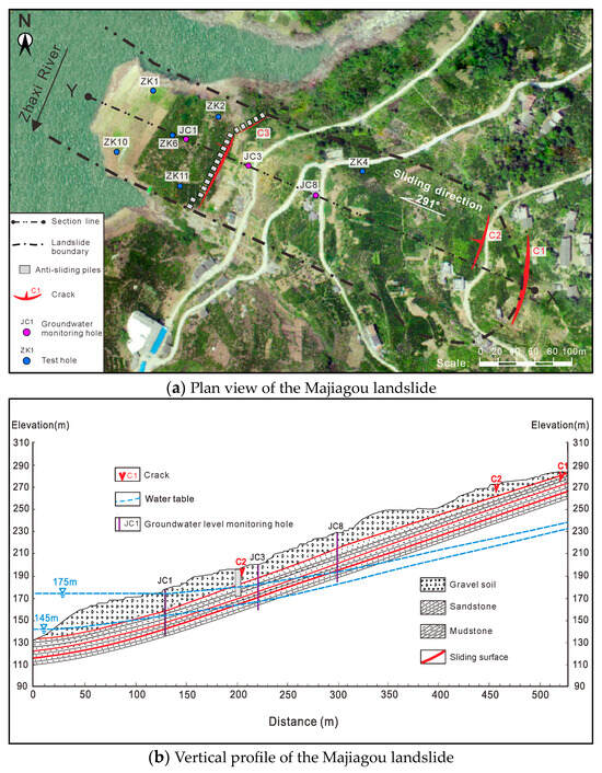
Figure 2.
Geological engineering and monitoring layout of the Majiagou landslide.
The bedrock in the landslide area mainly consists of gray-white feldspar quartz sandstone and fine sandstone, interbedded with purple-red siltstone and mudstone. These rocks are prone to weathering, and soften easily when exposed to water, making them highly susceptible to sliding in the Three Gorges area. The bedrock is characterized by developed fractures intersected by bedding planes, resulting in blocky, fragmented rocks that reduce the slope’s strength. Additionally, weak mudstone interlayers within the bedrock create favorable conditions for potential sliding surfaces.
To study the deformation and evolution characteristics of the Majiagou landslide, various monitoring instruments were installed at the landslide monitoring holes (JC), such as fiber optics, deep displacement, and water level gauges. Figure 2a,b illustrate the monitoring plan and engineering geological profile of the landslide, respectively.
Infiltration tests were conducted at several test holes (ZK) on the Majiagou landslide (distribution shown in Figure 2a) to obtain the permeability coefficients of the mass of landslide. The infiltration test results were shown in Table 1. However, as previously mentioned, the experimental results exhibit significant randomness and deviations, making them unsuitable for precise theoretical analysis and numerical simulation.

Table 1.
Infiltration test results for the Majiagou landslide.
3.2. Landslide GWL Monitoring
Inclinometers and water level gauges were installed in a series of boreholes (Figure 2). Inclinometers JC1 (40 m depth), JC3 (40 m depth), and JC8 (43 m depth) are positioned at elevations of 180 m, 198 m, and 225 m, respectively, with water level gauges installed at their bases. Figure 3 shows the GWL variations in three monitoring boreholes of the landslide in response to fluctuations in RWL. Rainfall has little effect on the fluctuation of GWL because the rainfall is less than 300 mm/month, and much of it becomes surface runoff rather than infiltrating the landslide.
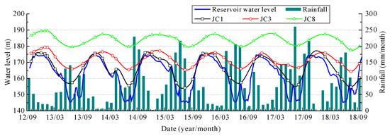
Figure 3.
Time series of GWL, RWL and rainfall.
According to the monitored results (Figure 3), the annual variations in GWL exhibited consistent patterns. Due to the high permeability of the surface deposits and the proximity of piezometer JC1 to the reservoir, the GWL at JC1 fluctuated synchronously with the reservoir level. However, the GWL at JC3 and JC8 lagged about two months behind the reservoir level decreases. However, monitored data can only reflect the changes in GWL at monitoring points in the landslide and cannot reflect the overall seepage field. Therefore, the following text will use an inverse analysis to obtain the permeability coefficient of the landslide and subsequently simulate the evolution law of the seepage field.
3.3. Establishment of the Landslide Seepage Field Model
3.3.1. Linear Fitting of the Reservoir Operation Cycle
Based on the 2010–2019 RWL data, a linear fitting curve of the reservoir operation cycle in the Three Gorges Reservoir area was established [34]. Thus, the hydraulic boundary conditions for transient analysis were set as variable head according to the linear fitting curve of the RWL (Figure 4a), and the calculation period was 1 year.
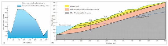
Figure 4.
Boundary conditions and seepage model for Simulation: (a) dynamic water head boundary; (b) seepage model for simulation.
3.3.2. Landslide Seepage Model
The main profile of the Majiagou landslide was selected, and a two-dimensional seepage model of the landslide was established based on the finite element program SEEP/W (Figure 4b). The horizontal width of the model was 650.0 m, and the vertical height was 292.0 m. The model was divided into triangular and quadrilateral meshes with 5329 mesh elements and 5217 nodes in total. The landslide model contained three different geological materials. Because rock fissures cannot be considered in the model calculation, the seepage of rock fissures was simplified into a seepage problem that was equivalent to a continuous medium. The left side was set as a variable head according to the generalized RWL model as Figure 4a shows, the bottom was set as an impermeable boundary, and the right-side boundary was set as a fixed head of 240 m. Three water level monitoring holes, S1, S3, and S8, were set on the landslide model, which corresponded to on-site monitoring boreholes JC1, JC3, and JC8.
3.3.3. Model Parameter Range
The model materials from top to bottom were gravel soil, fractured highly weathered rock, and moderately weathered bedrock. Due to the strong heterogeneity of the saturated permeability coefficient of gravel soil and complexity of the fracture development in the rock mass, the permeability coefficients in Table 1 obtained from the tests cannot be directly used for numerical calculations. Based on the results of permeability tests in boreholes and preliminary calculations of initial parameters using numerical models, this article established the order-of-magnitude range of permeability coefficients for three types of strata materials (see Table 2).
Table 2.
Range of permeability coefficients for landslide rock and soil materials.
4. Permeability Coefficient Inversion Based on LSSVM
4.1. Data Sample Construction
In theory, there are an infinite number of combinations of permeability coefficients for the three types of materials for a seepage inverse analysis. Calculating for each set of parameters would be difficult to implement and unnecessary. Therefore, this study adopts the design concept of uniform experimentation. A MATLAB R2021b program was used to generate 40 sets of data points in the range of (0, 1) (Table 3).
Table 3.
Normalized permeability coefficient list.
According to the range of the parameters to be inverted (Table 2), the combination samples of permeability coefficients can be obtained using the inverse normalization formula as follows:
where kimax and kimin are the upper and lower limits of the permeability coefficient range for the materials in Table 2, respectively. xij corresponds to the values in the (0, 1) interval in Table 3. Here, i = (1, 2, 3) and j = (1, 2, 3, …, 40).
The 40 sets of permeability coefficients k1, k2, and k3 obtained from the above inverse normalization process were input into the SEEP/W model, to calculate GWL after a RWL operation cycle. This step yielded 40 sets of simulated water levels of monitoring holes S1, S3, and S8. The simulated GWL were used as the input, and the permeability coefficients were used as the output for training. Subsequently, a sample set (Table 4) containing three columns of permeability coefficients and three columns of GWL was formed.
Table 4.
Simulated GWL and corresponding permeability coefficient sample data.
4.2. Training Effect and Inversion Predicted Values
The training samples data were imported into LSSVM, PSO-LSSVM, and WOA-LSSVM for learning and training. Finally, Table 5 shows the penalty factor C and kernel parameter determined after the optimization by each algorithm. The parameters of the standard LSSVM model were obtained by cross-validation and grid search, whereas the other two methods used swarm intelligence algorithms for 50 iterations of optimization. The graph of the relationship between iteration number and best fitness (Figure 5) shows that the best fitness after the 25th iteration was almost 0.0004 using the PSO optimization; with the WOA optimization, the fitness remained at approximately 0.0003 after only the 3rd iteration. Thus, the WOA is more efficient for this LSSVM parameter optimization problem.
Table 5.
Optimal parameters for LSSVM based on the three methods.
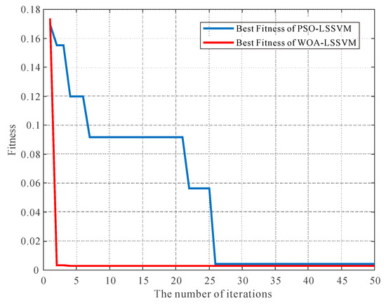
Figure 5.
Evolution of the optimal fitness curve for the optimization of LSSVM.
The relationship between the training values and predicted values of k1, k2, and k3 obtained through the PSO-LSSVM method is depicted in Figure 6, indicating excellent training performance. We used the coefficient of determination (R2) and the root mean square error (RMSE) as performance indicators [11] to evaluate the fitting effectiveness of sample data for the model. As shown in Table 6, the R2 values of the three methods were all very close to 1 and the RMSE values were relatively small, which indicates good fitting effects. Among them, the WOA-LSSVM prediction model achieved the best fitting effect.
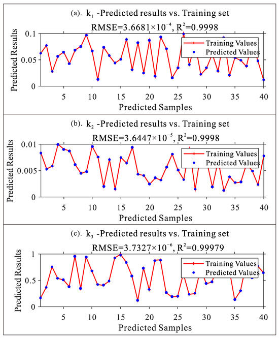
Figure 6.
PSO-LSSVM training effectiveness. (a) k1 predicted results; (b) k2 predicted results; (c) k3 predicted results.
Table 6.
Permeability coefficient inverse values, training performance RMSE and R2.
During the low water level operation period, the average monitored GWL (data from the year 2012 to 2018 in Figure 3) at each monitoring boreholes were as follows: JC1: 155.83 m; JC3: 165.57 m; JC8: 179.65 m. Then, this set of monitoring data were used as test values to invert the landslide permeability coefficients using three different algorithms. Table 6 shows the inverse values of the permeability coefficients.
Subsequently, the inversion values obtained from the three methods were input into the finite element model to calculate the simulated GWL of the landslide, as shown in Table 7. Introducing a relative error to evaluate the inversion effectiveness, we observe that all inversion calculations of the three algorithms had relatively small relative errors, which satisfies the accuracy requirements for permeability calculations. Specifically, the PSO-LSSVM algorithm achieved the best inversion performance, followed by LSSVM, and WOA-LSSVM was slightly inferior. Thus, WOA-LSSVM is prone to premature convergence or overfitting during training, which results in relatively larger relative errors in the inversion calculations.
Table 7.
Simulated GWL and their relative errors compared to the monitored values.
5. Analysis of the Seepage Field in a Landslide
5.1. Comparison of the Simulated and Monitored Water Levels
Based on the permeability coefficients obtained from the PSO-LSSVM inversion, the continuous variation in GWL throughout the entire operational cycle of the reservoir was simulated. The average measured GWL of 2012–2018 at the monitoring points of the landslide were compared with the simulated values, as shown in Figure 7a. The measured GWL at the monitoring points of the landslide were very similar to the simulated values, which indicates that the inversion results are relatively reliable. The inversion method based on PSO-LSSVM demonstrates good effectiveness and accuracy.
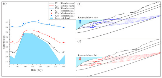
Figure 7.
Seepage field results of the Majiagou landslide: (a) comparison of the average measured GWL and simulated values; (b) variation in groundwater lines during reservoir rising stage; (c) variation in groundwater lines during reservoir falling stage.
5.2. Evolution Characteristics of the Seepage Field
The characteristics of the seepage of the landslide under fluctuating RWL were computed using the inversion permeability coefficients. The groundwater infiltration line changed over time in the RWL rise phase (Figure 7b) and the decline phase (Figure 7c). The following observations were made.
- Given the relatively high permeability coefficient of gravelly soil, the frontal infiltration line of the landslide synchronously rose and fell with the RWL, and the fluctuation range of the infiltration line gradually decreased from front to back.
- During the rising stage of the RWL [30–90 days], as depicted in Figure 7b, the infiltration line began to concave toward the slope on approximately 50th days, which indicates a lag in the rise of GWL within the slope compared to the RWL. Subsequently, on 90th days, the RWL rose to 174 m, and a significant lag in the infiltration line appeared at the interface of the two materials. Until approximately 150 days, the infiltration line in the slope reached its peak GWL with a lag time of approximately 60 days. During the reservoir water storage process, the seepage field belonged to the inward recharge type, and the infiltration line concaved toward the slope, and an infiltration pressure formed toward the slope, which was conducive to landslide stability.
- During the falling stage of the RWL [150–300 days], as shown in Figure 7b, with decreasing water level, the frontal infiltration line of the landslide remained horizontal with the RWL, and the inclination angle of the midsection infiltration line gradually increased. During the rapid decline stage of the RWL [250–300 days], the rate of change in inclination angle increased, and the slope of the infiltration line significantly increased. The increasing inclination angle of the infiltration line indicates a gradual increase in hydraulic head difference between front and rear parts of the landslide, which increased the infiltration pressure within the slope towards the reservoir and reduced the landslide stability.
6. Discussion
The permeability coefficient is a crucial parameter to study the reservoir slope stability and deformation. When using the permeability coefficients obtained from infiltration tests (Table 1) for seepage simulation, we encountered two issues: firstly, the test results themselves had significant deviations, making it difficult to determine which test value to use; secondly, the simulation trial calculations were found to be completely inconsistent with the actual situation. The proposed method in this paper to inversely estimate the permeability coefficients of a landslide mass has advantages such as accuracy, efficiency, and low requirement for monitoring data samples. The use of dynamic hydraulic boundary conditions in finite element transient analysis helps to better match the simulation results with actual conditions.
However, the monitored frequency of GWL in this landslide case was relatively low, so extreme points of water level data changes might have been missed, which would affect the inversion results. Additionally, rainfall may temporarily elevate water levels within the monitoring holes and affected the final inversion results. In the future, efforts will be made to enhance the continuity and accuracy of monitoring data and conduct further research.
Further, due to the drawbacks of LSSVM, such as sensitivity to noise and parameter selection, which may impact the study results. We plan to expand our research approach and methods in future studies by selecting more additional algorithms for comparative analysis.
7. Conclusions
In this study, a method to inversely estimate the permeability coefficient of a landslide mass using GWL monitoring data was proposed. The Majiagou landslide in the Three Gorges Reservoir area was used as an example. The permeability coefficients of the landslide were obtained through field monitoring, finite element simulation, and machine learning. The verification results matched the field monitoring results. The following conclusions were drawn.
- The feasibility of using LSSVM for the inversion of landslide permeability coefficients has been well validated. Additionally, it has been confirmed that training data generated from finite element transient analysis of seepage can be used to accurately invert permeability coefficients.
- LSSVM, PSO-LSSVM, and WOA-LSSVM were effective in fitting the nonlinear relationship between landslide permeability coefficient and GWL. Among them, the WOA-optimized LSSVM algorithm had the highest efficiency and fitting degree. However, during the inversion process, PSO-LSSVM had the smallest error and best inversion effect, whereas WOA-LSSVM had the largest error and a slightly poorer inversion effect. Therefore, multiple methods should be compared to select the best parameter inversion values.
- The PSO-LSSVM inversion obtained the following permeability coefficients of the Majiagou landslide mass: gravelly soil k1 = 4.385 × 10⁻² cm/s; highly weathered fractured rock k2 = 5.819 × 10⁻³ cm/s; mid-weathered rock k3 = 6.284 × 10⁻⁴ cm/s. Inputting these values into the model to simulate GWL yielded simulated values that closely matched the measured values, thus indicating the high reliability of the inversion results and strong feasibility of the method. Additionally, this method could be extended to the inversion analysis of deformation parameters and strength parameters of a landslide mass.
This study will facilitate subsequent fluid–solid coupling analyses of landslides, offering a foundation for a deeper understanding of the mechanisms driving landslide evolution. Thus, it will provide a theoretical basis for accurately predicting and effectively preventing reservoir landslides.
Author Contributions
Conceptualization, X.T.; methodology, X.T. and C.S.; software, X.T. and Y.Z.; validation, X.T. and C.S.; formal analysis, X.T.; investigation, Y.Z.; resources, Y.Z.; data curation, Y.Z.; writing—original draft preparation, X.T.; writing—review and editing, C.S. All authors have read and agreed to the published version of the manuscript.
Funding
This work was supported by the National Natural Science Foundation of China (Grant No. 52379100 and 41831278).
Institutional Review Board Statement
Not applicable.
Informed Consent Statement
Not applicable.
Data Availability Statement
The water level data of the Three Gorges Reservoir can be accessed from the website of Three Gorges Navigation Authority. The website link is https://sxth.mot.gov.cn/sj/, accessed on 1 May 2024. The MATLAB codes for study are available upon reasonable request to the corresponding author.
Acknowledgments
The authors would like to thank the research group of Xinli Hu at China University of Geosciences, for their contributions to the field experiments on the Majiagou landslide, as well as for providing data and assistance for this study.
Conflicts of Interest
The authors declare that they have no competing interests.
References
- Yin, Y.; Wang, L.; Zhang, W.; Zhang, Z.; Dai, Z. Research on the collapse process of a thick-layer dangerous rock on the reservoir bank. Bull. Eng. Geol. Environ. 2022, 81, 109. [Google Scholar] [CrossRef]
- Tang, H.; Wasowski, J.; Juang, C.H. Geohazards in the Three Gorges Reservoir area, China–lessons learned from decades of research. Eng. Geol. 2019, 261, 105267. [Google Scholar] [CrossRef]
- Hu, X.; Zhang, M.; Sun, M.; Huang, K.; Song, Y. Deformation characteristics and failure mode of the zhujiadian landslide in the Three Gorges Reservoir, China. Bull. Eng. Geol. Environ. 2015, 74, 1–12. [Google Scholar] [CrossRef]
- Zhou, C.; Shao, W.; van Westen, C.J. Comparing two methods to estimate lateral force acting on stabilizing piles for a landslide in the Three Gorges Reservoir, China. Eng. Geol. 2014, 173, 41–53. [Google Scholar] [CrossRef]
- Wen, Z.; Zhan, H.; Wang, Q.; Liang, X.; Ma, T.; Chen, C. Well hydraulics in pumping tests with exponentially decayed rates of abstraction in confined aquifers. J. Hydrol. 2017, 548, 40–45. [Google Scholar] [CrossRef]
- Dewandel, B.; Lanini, S.; Lachassagne, P.; Maréchal, J.-C. A generic analytical solution for modelling pumping tests in wells intersecting fractures. J. Hydrol. 2018, 559, 89–99. [Google Scholar] [CrossRef]
- Basile, A.; Ciollaro, G.; Coppola, A. Hysteresis in soil water characteristics as a key to interpreting comparisons of laboratory and field measured hydraulic properties. Water Resour. Res. 2003, 39, 1355. [Google Scholar] [CrossRef]
- Farcas, A.; Elliott, L.; Ingham, D.B.; Lesnic, D. An inverse dual reciprocity method for hydraulic conductivity identification in steady groundwater flow. Adv. Water Resour. 2004, 27, 223–235. [Google Scholar] [CrossRef]
- Deng, J.H.; Lee, C.F. Displacement back analysis for a steep slope at the three gorges project site. Int. J. Rock Mech. Min. Sci. 2001, 38, 259–268. [Google Scholar] [CrossRef]
- Kazemi, F.; Asgarkhani, N.; Jankowski, R. Machine learning-based seismic fragility and seismic vulnerability assessment of reinforced concrete structures. Soil Dyn. Earthq. Eng. 2023, 166, 107761. [Google Scholar] [CrossRef]
- Kazemi, F.; Asgarkhani, N.; Jankowski, R. Machine learning-based seismic response and performance assessment of reinforced concrete buildings. Arch. Civ. Mech. Eng. 2023, 23, 94. [Google Scholar] [CrossRef]
- Sun, G.; Zheng, H.; Huang, Y.; Li, C. Parameter inversion and deformation mechanism of sanmendong landslide in the Three Gorges Reservoir region under the combined effect of reservoir water level fluctuation and rainfall. Eng. Geol. 2016, 205, 133–145. [Google Scholar] [CrossRef]
- Liang, Z.; Gong, B.; Tang, C.; Zhang, Y.; Ma, T. Displacement back analysis for a high slope of the dagangshan hydroelectric power station based on bp neural network and particle swarm optimization. Sci. World J. 2014, 2014, 741323. [Google Scholar] [CrossRef] [PubMed]
- Zhuang, D.Y.; Ma, K.; Tang, C.A.; Liang, Z.Z.; Wang, K.K.; Wang, Z.W. Mechanical parameter inversion in tunnel engineering using support vector regression optimized by multi-strategy artificial fish swarm algorithm. Tunn. Undergr. Space Technol. 2019, 83, 425–436. [Google Scholar] [CrossRef]
- Chang, X.; Wang, H.; Zhang, Y. Back analysis of rock mass parameters in tunnel engineering using machine learning techniques. Comput. Geotech. 2023, 163, 105738. [Google Scholar] [CrossRef]
- Li, H.; Chen, W.; Tan, X.; Tan, X. Back analysis of geomechanical parameters for rock mass under complex geological conditions using a novel algorithm. Tunn. Undergr. Space Technol. 2023, 136, 105099. [Google Scholar] [CrossRef]
- Wang, S.; Xu, B.; Zhu, Z.; Li, J.; Lu, J. Reliability analysis of concrete gravity dams based on least squares support vector machines with an improved particle swarm optimization algorithm. Appl. Sci. 2022, 12, 12315. [Google Scholar] [CrossRef]
- Zhou, C.-B.; Liu, W.; Chen, Y.-F.; Hu, R.; Wei, K. Inverse modeling of leakage through a rockfill dam foundation during its construction stage using transient flow model, neural network and genetic algorithm. Eng. Geol. 2015, 187, 183–195. [Google Scholar] [CrossRef]
- Ren, J.; Shen, Z.-Z.; Yang, J.; Yu, C.-Z. Back analysis of the 3d seepage problem and its engineering applications. Environ. Earth Sci. 2016, 75, 113. [Google Scholar] [CrossRef]
- Fei, T.; Anan, Z.; Jie, Y.; Lin, C. Inversion analysis of rock mass permeability coefficient of dam engineering based on particle swarm optimization and support vector machine: A case study. Measurement 2023, 221, 113580. [Google Scholar] [CrossRef]
- Yu, J.a.; Shen, Z.; Li, H.; Li, F.; Huang, Z. An artificial intelligence optimization method of back analysis of unsteady-steady seepage field for the dam site under complex geological condition. Bull. Eng. Geol. Environ. 2024, 83, 127. [Google Scholar] [CrossRef]
- Wang, Y. Application of the Improved Support Vector Machine in Slope Stability Evaluation and Parameter Inversion. Master’s Thesis, China University of Geosciences, Beijing, China, 2014. [Google Scholar]
- Das, S.K.; Samui, P.; Sabat, A.K. Prediction of field hydraulic conductivity of clay liners using an artificial neural network and support vector machine. Int. J. Geomech. 2012, 12, 606–611. [Google Scholar] [CrossRef]
- Thomas, A.; Majumdar, P.; Eldho, T.I.; Rastogi, A.K. Simulation optimization model for aquifer parameter estimation using coupled meshfree point collocation method and cat swarm optimization. Eng. Anal. Bound. Elem. 2018, 91, 60–72. [Google Scholar] [CrossRef]
- Yue, X.; Wang, Y.; Wen, T. An inversion study of reservoir colluvial landslide permeability coefficient by combining physical model and data-driven models. Water 2024, 16, 686. [Google Scholar] [CrossRef]
- Wang, Y.J.; Wang, Q.; Cao, Y.B. The inversion analysis of the reservoir saturation landslide’s permeability coefficient. Appl. Mech. Mater. 2014, 490, 633–639. [Google Scholar] [CrossRef]
- Li, Y.; Yang, J.; Cheng, L.; Ma, C. Inversion analysis on permeability coefficient of stratum in engineering area based on rvm-cs. J. Yangtze River Sci. Res. Inst. 2020, 37, 121. (In Chinese) [Google Scholar]
- Samui, P.; Kothari, D.P. Utilization of a least square support vector machine (lssvm) for slope stability analysis. Sci. Iran. 2011, 18, 53–58. [Google Scholar] [CrossRef]
- Samui, P. Application of least square support vector machine (lssvm) for determination of evaporation losses in reservoirs. Engineering 2011, 334049, 431–434. [Google Scholar] [CrossRef]
- Ding, Y.; Zhao, J.; Yuan, Z.Y.; Zhang, Y.; Xiong, L. Constrained surface recovery using rbf and its efficiency improvements. J. Multimed. 2010, 5, 55–62. [Google Scholar]
- Eberhart, R.; Kennedy, J. Particle swarm optimization. In Proceedings of the IEEE International Conference on Neural Networks, Perth, WA, Australia, 27 November–1 December 1995; Citeseer: Princeton, NI, USA, 1995; Volume 4, pp. 1942–1948. [Google Scholar]
- Mirjalili, S.; Lewis, A. The whale optimization algorithm. Adv. Eng. Softw. 2016, 95, 51–67. [Google Scholar] [CrossRef]
- Zhang, Y.; Hu, X.; Tannant, D.D.; Zhang, G.; Tan, F. Field monitoring and deformation characteristics of a landslide with piles in the Three Gorges Reservoir area. Landslides 2018, 15, 581–592. [Google Scholar] [CrossRef]
- Yin, Y.P.; Zhang, C.Y.; Yan, H.; Xiao, M.; Hou, X.; Zhu, S. Research on seepage stability and prevention design of landslide during impoundment operation of the Three Gorges Reservoir, China. Chin. J. Rock Mech. Eng. 2021, 41, 649–659. (In Chinese) [Google Scholar]
Disclaimer/Publisher’s Note: The statements, opinions and data contained in all publications are solely those of the individual author(s) and contributor(s) and not of MDPI and/or the editor(s). MDPI and/or the editor(s) disclaim responsibility for any injury to people or property resulting from any ideas, methods, instructions or products referred to in the content. |
© 2024 by the authors. Licensee MDPI, Basel, Switzerland. This article is an open access article distributed under the terms and conditions of the Creative Commons Attribution (CC BY) license (https://creativecommons.org/licenses/by/4.0/).