

Shape Control of a Carbon Fiber-Reinforced Polymer Reflector and Placement Optimization of the Actuators

Abstract
1. Introduction
2. Materials and Methods
2.1. Displacements and Strain Assumption
2.2. Constitutive Equations
2.3. Interpolation Formulation
2.4. Variation Formulation
3. Results
4. Optimal Placement of PZT Actuators
4.1. Basic Strategies of Genetic Algorithm for Actuator Placement Optimization
4.2. Implementation of Genetic Algorithm for Single-Objective Optimization
- Case 1: Displacement load consists of Zernike polynomials
- Numerical example
- 2.
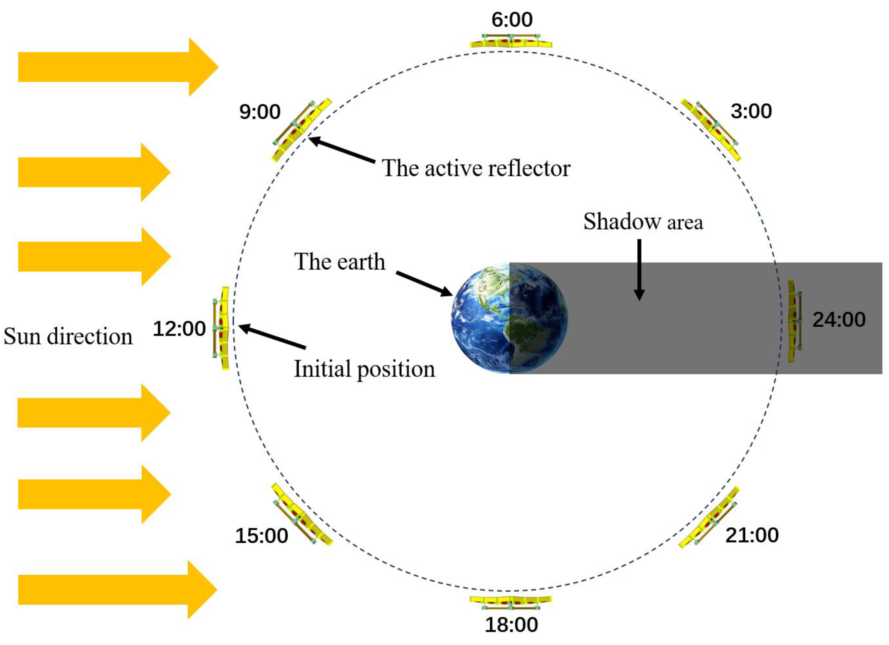
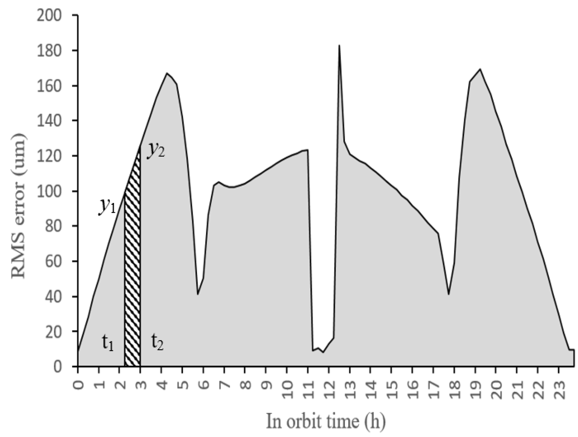
- In-orbit thermal load
- Numerical example
4.3. Implementation of Genetic Algorithm for Multi-Objective Optimization
- Numerical examples
4.4. Discussion
5. Conclusions
Author Contributions
Funding
Institutional Review Board Statement
Informed Consent Statement
Data Availability Statement
Conflicts of Interest
Appendix A
References
- Pearson, J.; Moore, J.; Fang, H. Large and High Precision Inflatable Membrane Reflector. In Proceedings of the 51st AIAA/ASME/ASCE/AHS/ASC Structures, Structural Dynamics, and Materials Conference, 18th AIAA/ASME/AHS Adaptive Structures Conference, Orlando, FL, USA, 12–15 April 2010. [Google Scholar]
- Lang, M.; Baier, H.; Ernst, T. High Precision Thin Shell Reflectors-Design Concepts, Structural Optimisation and Shape Adjustment Techniques. In Proceedings of the European Conference on Spacecraft Structures, Materials and Mechanical Testing 2005 (ESA SP-581), Noordwijk, The Netherlands, 10–12 May 2005; Volume 581, p. 11.1. [Google Scholar]
- Shi, H.; Yuan, S.; Yang, B. New Methodology of Surface Mesh Geometry Design for Deployable Mesh Reflectors. J. Spacecr. Rocket. 2018, 55, 266–281. [Google Scholar] [CrossRef]
- Yuan, S.; Yang, B.; Fang, H. The Projecting Surface Method for Improvement of Surface Accuracy of Large Deployable Mesh Reflectors. Acta Astronaut. 2018, 151, 678–690. [Google Scholar] [CrossRef]
- Yuan, S.; Yang, B.; Fang, H. Enhancement of Large Deployable Mesh Reflectors by the Self-Standing Truss with Hard-Points. In Proceedings of the AIAA Scitech 2019 Forum, San Diego, CA, USA, 7 January 2019. [Google Scholar]
- Yuan, S.; Yang, B.; Fang, H. Self-Standing Truss with Hard-Point-Enhanced Large Deployable Mesh Reflectors. AIAA J. 2019, 57, 5014–5026. [Google Scholar] [CrossRef]
- Soykasap, O.; Tan, L.T. High-Precision Offset Stiffened Springback Composite Reflectors. AIAA J. 2011, 49, 2144–2151. [Google Scholar] [CrossRef]
- Tabata, M.; Natori, M.C. Active Shape Control of a Deployable Space Antenna Reflector. J. Intell. Mater. Syst. Struct. 1996, 7, 235–240. [Google Scholar] [CrossRef]
- Welch, S.S. A Distributed Sensor and Processor for Surface Control of a Large Reflector. In Proceedings of the IEEE Proceedings on Southeastcon, New Orleans, LA, USA, 1–4 April 1990; pp. 122–125. [Google Scholar]
- Wang, Z.; Li, T.; Deng, H. Form-Finding Analysis and Active Shape Adjustment of Cable Net Reflectors with PZT Actuators. J. Aerosp. Eng. 2014, 27, 575–586. [Google Scholar] [CrossRef]
- Stein, G.; Gorinevsky, D. Design of Surface Shape Control for Large Two-Dimensional Arrays. IEEE Trans. Contr. Syst. Technol. 2005, 13, 422–433. [Google Scholar] [CrossRef]
- Andoh, F.; Washington, G.; Yoon, H.-S.; Utkin, V. Efficient Shape Control of Distributed Reflectors with Discrete Piezoelectric Actuators. J. Intell. Mater. Syst. Struct. 2004, 15, 3–15. [Google Scholar] [CrossRef]
- Lu, Y.-F.; Yue, H.-H.; Deng, Z.-Q.; Tzou, H.-S. Research on Active Control for Thermal Deformation of Precise Membrane Reflector With Boundary SMA Actuators. In Proceedings of the Volume 4B: Dynamics, Vibration, and Control; American Society of Mechanical Engineers, Montreal, QC, Canada, 14 November 2014; p. V04BT04A061. [Google Scholar]
- DeSmidt, H.A.; Wang, K.W.; Fang, H. Optimized Gore/Seam Cable Actuated Shape Control of Gossamer Membrane Reflectors. J. Spacecr. Rocket. 2007, 44, 1122–1130. [Google Scholar] [CrossRef]
- Suleman, A.; Gonicalves, M.A. Multi-Objective Optimization of an Adaptive Composite Beam Using the Physical Programming Approach. J. Intell. Mater. Syst. Struct. 1999, 10, 56–70. [Google Scholar] [CrossRef]
- Adali, S.; Bruch, J.C., Jr.; Sadek, I.S.; Sloss, J.M. Robust Shape Control of Beams with Load Uncertainties by Optimally Placed Piezo Actuators. Struct. Multidiscip. Optim. 2000, 19, 274–281. [Google Scholar] [CrossRef]
- Aldraihem, O.J.; Singh, T.; Wetherhold, R.C. Optimal Size and Location of Piezoelectric Actuator/Sensors: Practical Considerations. J. Guid. Control Dyn. 2000, 23, 509–515. [Google Scholar] [CrossRef]
- Barboni, R.; Mannini, A.; Fantini, E.; Gaudenzi, P. Optimal Placement of PZT Actuators for the Control of Beam Dynamics. Smart Mater. Struct. 2000, 9, 110–120. [Google Scholar] [CrossRef]
- Bruant, I.; Coffignal, G.; Lene, F.; Verge, M. A Methodology for Determination of Piezoelectric Actuator and Sensor Location on Beam Structures. J. Sound Vib. 2001, 243, 861–882. [Google Scholar] [CrossRef]
- Dong, Y.; Huang, H. Truss Topology Optimization by Using Multi-Point Approximation and GA. Chin. J. Comput. Mech. 2004, 21, 746–751. [Google Scholar]
- An, H.; Xian, K.; Huang, H. Actuator Placement Optimization for Adaptive Trusses Using a Two-Level Multipoint Approximation Method. Struct. Multidisc Optim 2016, 53, 29–48. [Google Scholar] [CrossRef]
- Liu, S.; Lin, Z. Integrated Design Optimization of Voltage Channel Distribution and Control Voltages for Tracking the Dynamic Shapes of Smart Plates. Smart Mater. Struct. 2010, 19, 125013. [Google Scholar] [CrossRef]
- Honda, S.; Kajiwara, I.; Narita, Y. Multidisciplinary Design Optimization for Vibration Control of Smart Laminated Composite Structures. J. Intell. Mater. Syst. Struct. 2011, 22, 1419–1430. [Google Scholar] [CrossRef]
- DeLorenzo, M.L. Sensor and Actuator Selection for Large Space Structure Control. J. Guid. Control Dyn. 1990, 13, 249–257. [Google Scholar] [CrossRef]
- Kuo, C.-P.; Bruno, R. Optimal Actuator Placement on an Active Reflector Using a Modified Simulated Annealing Technique. In Proceedings of the Japan Conference on Adaptive Structures, Maui, HI, USA, 13–15 November 1991; pp. 1056–1067. [Google Scholar]
- Sheng, L.; Kapania, R.K. Genetic Algorithms for Optimization of Piezoelectric Actuator Locations. AIAA J. 2001, 39, 1818–1822. [Google Scholar] [CrossRef]
- Hill, J.R.; Wang, K.W.; Fang, H.; Quijano, U. Actuator Grouping Optimization on Flexible Space Reflectors. In Proceedings of the SPIE the International Society for Optical Engineering, San Diego, CA, USA, 24 March 2011; Ghasemi-Nejhad, M.N., Ed.; Springer: Berlin/Heidelberg, Germany, 2011; p. 797725. [Google Scholar]
- Wang, Z.; Cao, Y.; Zhao, Y.; Wang, Z. Modeling and Optimal Design for Static Shape Control of Smart Reflector Using Simulated Annealing Algorithm. J. Intell. Mater. Syst. Struct. 2016, 27, 705–720. [Google Scholar] [CrossRef]
- Lan, L.; Jiang, S.; Zhou, Y.; Fang, H.; Wu, Z.; Du, J. Shape Control of a Reflector Based on Generalized Zernike Functions. In Proceedings of the 3rd AIAA Spacecraft Structures Conference; American Institute of Aeronautics and Astronautics, San Diego, CA, USA, 4 January 2016. [Google Scholar]
- Reddy, J.N. On Laminated Composite Plates with Integrated Sensors and Actuators. Eng. Struct. 1999, 21, 568–593. [Google Scholar] [CrossRef]
- Wu, K.; Fang, H. Suppressing High-Order Surface Errors of an Active Carbon Fiber Reinforced Composite Reflector Using Two Types of Actuators. Opt. Eng. 2019, 58, 1. [Google Scholar] [CrossRef]
- Ren, Z.W.; San, Y. Improved Adaptive Genetic Algorithm and Its Application Research in Parameter Identification. J. Syst. Simul. 2006, 18, 41–43. [Google Scholar]
- Zhao, C.; Burge, J.H. Orthonormal Vector Polynomials in a Unit Circle, Part I: Basis Set Derived from Gradients of Zernike Polynomials. Opt. Express 2007, 15, 18014. [Google Scholar] [CrossRef] [PubMed]
- Gilmore, D.G. Spacecraft Thermal Control Handbook: Cryogenics; AIAA: Las Vegas, NV, USA, 2002; Volume 2, ISBN 1-884989-14-4. [Google Scholar]
- Duan, B.; Gao, F.; Du, J.; Zhang, S. Optimization and Experiment of an Electrostatic Forming Membrane Reflector in Space. J. Mech. Sci Technol 2015, 29, 1355–1360. [Google Scholar] [CrossRef]
- Dhuri, K.D.; Seshu, P. Multi-Objective Optimization of Piezo Actuator Placement and Sizing Using Genetic Algorithm. J. Sound Vib. 2009, 323, 495–514. [Google Scholar] [CrossRef]
- Figueira, J.; Greco, S.; Ehrgott, M. Multiple Criteria Decision Analysis: State of the Art Surveys; Springer Science & Business Media: Berlin/Heidelberg, Germany, 2005; ISBN 038723067X. [Google Scholar]


| Materials | Property | Value | |
|---|---|---|---|
| Unidirectional carbon fiber layer | Elastic modulus | E1 (GPa) | 145 |
| E2 (GPa) | 11 | ||
| Poisson’s ratio | v12 | 0.25 | |
| Shear modulus | G12 (GPa) | 5.28 | |
| G13 (GPa) | 5.28 | ||
| G23 (GPa) | 4.23 | ||
| PZT actuators’ equivalent parameters | Elastic modulus | E1 (GPa) | 26.53 |
| Shear modulus | τzx (GPa) | 2.15 | |
| Maximum voltages (V) | 150 | ||
| Minimum voltages (V) | −100 | ||
| Equivalent length (mm) | 80 | ||
| Poisson’s ratio | 0.3 | ||
| Piezoelectric constant (pm/V) | 360 | ||
| Structural Parameter | Value |
|---|---|
| Inscribed circle diameter of the outermost grille | 1.0 m |
| Focal length | 2.1 m |
| Width of the grid | 0.1886 m |
| Height of the grid | 0.06 m |
| Excavation width of grid | 0.1 m |
| Depth of the grid | 0.02 m |
| Property | Value | ||
|---|---|---|---|
| Materials | Single-fiber layer prepreg | PZT actuator (average) | |
| Thermal Conductivity (W/m K) | 18.6 | 37.2 | |
| Specific Heat (J/kg·K) | 850 | 460 | |
| CTE (/°C) | −1.01 × 10⁻⁶ | 3.81 × 10⁻⁶ | 8.00 × 10⁻⁶ |
| Density (kg/m3) | 1510 | 5060 | |
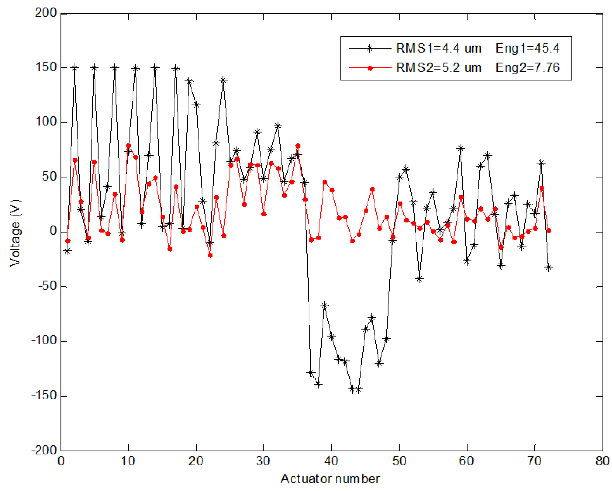
| Value of Objectives | Single RMS Error Optimization (µm) | |||||||
|---|---|---|---|---|---|---|---|---|
| f1 | 4.4 | |||||||
| f2 | 45.4 | |||||||
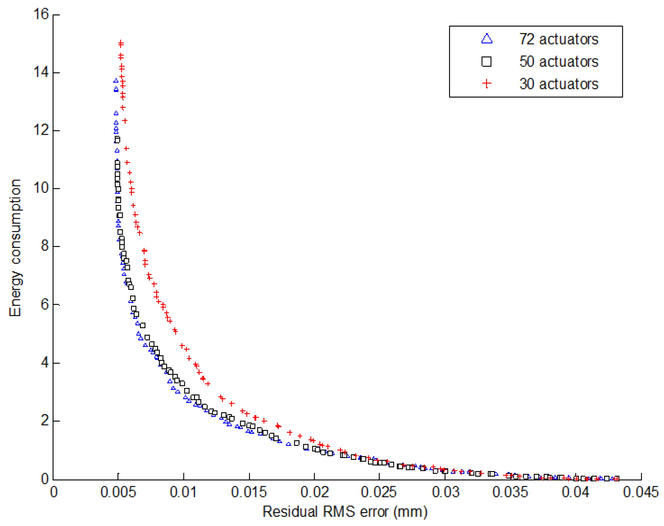
| Value of Objectives | Residual RMS Error (µm) and Energy Consumption | |||||||
| f1 | 4.9 | 5.2 | 5.4 | 5.8 | 5.4 | 6.2 | 7.0 | 7.9 |
| f2 | 9.1 | 7.8 | 6.9 | 6.0 | 7.3 | 5.5 | 4.7 | 3.8 |
| Value of Objectives | Residual RMS Error (µm) and Energy Consumption | |||||||
| f1 | 8.5 | 10.6 | 12.7 | 15.0 | 17.8 | 21.7 | 28.0 | |
| f2 | 3.4 | 2.7 | 2.1 | 1.7 | 1.3 | 0.88 | 0.42 | |
Disclaimer/Publisher’s Note: The statements, opinions and data contained in all publications are solely those of the individual author(s) and contributor(s) and not of MDPI and/or the editor(s). MDPI and/or the editor(s) disclaim responsibility for any injury to people or property resulting from any ideas, methods, instructions or products referred to in the content. |
© 2024 by the authors. Licensee MDPI, Basel, Switzerland. This article is an open access article distributed under the terms and conditions of the Creative Commons Attribution (CC BY) license (https://creativecommons.org/licenses/by/4.0/).
Share and Cite
Wu, K.; Yang, W.; Liu, P. Shape Control of a Carbon Fiber-Reinforced Polymer Reflector and Placement Optimization of the Actuators. Appl. Sci. 2024, 14, 4765. https://doi.org/10.3390/app14114765
Wu K, Yang W, Liu P. Shape Control of a Carbon Fiber-Reinforced Polymer Reflector and Placement Optimization of the Actuators. Applied Sciences. 2024; 14(11):4765. https://doi.org/10.3390/app14114765
Chicago/Turabian StyleWu, Ke, Wenhai Yang, and Pengbo Liu. 2024. "Shape Control of a Carbon Fiber-Reinforced Polymer Reflector and Placement Optimization of the Actuators" Applied Sciences 14, no. 11: 4765. https://doi.org/10.3390/app14114765
APA StyleWu, K., Yang, W., & Liu, P. (2024). Shape Control of a Carbon Fiber-Reinforced Polymer Reflector and Placement Optimization of the Actuators. Applied Sciences, 14(11), 4765. https://doi.org/10.3390/app14114765