Featured Application
Results provide essential information for the initial design and adaptation potential of Nature-Based Solutions. It may serve as guidance to practitioners and data providers.
Abstract
Flooding events, like in Germany in 2021, highlight the need for re-naturalising banks of rivers and streams to naturally mitigate future flooding. To identify potential areas for Nature-Based Solutions (NBS), the NBS Toolkit—a decision-support tool for Europe—was developed within the H2020 OPERANDUM project. The tool builds on suitability mapping, which is progressively adopted for pre-assessing areas for Nature-Based Solutions. The NBS Toolkit operates with European open-source data, which is available at different spatial resolutions. In this study, we performed a GIS-based analysis to examine the impact of different resolution data on the resulting suitability maps. The results suggest that for large-scale measures such as riparian forest buffers, coarser resolutions are sufficient and may save processing time and capacities. However, fine resolution datasets can bring added value to urban suitability mapping and are of greater importance for small-scale, local Nature-Based Solutions.
1. Introduction
Nature-Based Solutions (NBS) have been gaining a significant role in disaster risk reduction, climate change mitigation and adaptation, as well as in sustainable development [1]. Their rising importance in policies and practice in Europe can be ascribed to their character as natural measures which simultaneously offer co-benefits for the socio-ecological system [2,3].
The increasing recognition of NBS in Europe is linked to the ambition to implement them at various scales in rural and urban areas [4]. To enhance the uptake of NBS, it is necessary to support the decision-making of policy makers, practitioners, associations, and further actors who are not experts in this field but are engaged in the planning and implementation of NBS because they have specific requirements (e.g., for soil) that need to be considered. Hence, to determine the suitability of a particular NBS for an area of interest, several criteria need to be fulfilled. For decision-support, a preliminary assessment can be conducted based on local characteristics (e.g., soil, land cover, vegetation, and built-up areas) to gain an initial understanding of the suitability of an NBS. This type of multi-criteria pre-assessment in NBS is referred to as suitability mapping [5], (site) suitability analysis/assessment [6], or, alternatively, as opportunity mapping [7]. When conducting a complete suitability analysis for real-world application, several additional criteria which are not covered in the pre-assessment may also need to be considered. These additional criteria may be social aspects (e.g., acceptance of the NBS by the public), legal factors (e.g., land ownership, policies in context of the permission of NBS), and the economic component (e.g., funding for the land reimbursement, implementation, and maintenance) [5,8,9,10,11].
Existing suitability mapping tools and studies vary in their scale, although the following core approach remains similar: focus on urban areas and city scale [11], perform subnational scale analysis primarily for rural areas [12], map NBS suitability at a larger scale (e.g., national) [5], and at a global scale [7]. However, NBS suitability mapping has not been approached at the European level yet. In response to this gap and the increasing promotion of NBS in Europe, as well as the complexity of decision-making for NBS, we developed the NBS Toolkit [13] (within the H2020 OPERANDUM project) to support decision-making for NBS in rural and urban areas. The NBS Toolkit aims to recommend NBS locations for the entire European region at the local scale. The suitability mapping of the toolkit builds on open-source data at the European scale, but the available datasets can vary greatly in resolution. For instance, datasets for land use and land cover (LULC) are available in 100 m, 50 m, and down to 2 m resolution. In order to gain evidence on the appropriateness of these different open-source datasets for the suitability mapping at the regional scale, this study aims to assess the influence of different spatial resolutions on the resulting suitability maps.
Differences in spatial resolution can be further related to differences in accuracy and data size, and have been found to impact the computation outcome, i.e., in the context of hydrological modelling [14,15,16,17,18], ecosystem service assessments [19,20], or agricultural suitability mapping [21]. These studies discussed the result accuracy, the adequateness of fine resolution in the context of the desired goal of a study, and the feasibility of fine resolution, considering computation capacity. In terms of accuracy of the results, it was found that accuracy increases equally with finer spatial resolution [19], provided that all input layers are of a similar resolution [15]. Considering the desired output scale, fine spatial resolution could be a precondition, i.e., for urban suitability mapping due to greater land use heterogeneity [19]. Hence, which output scale is desired should be considered [18]. Other selection factors for input layers are the availability of data, the computation resources (e.g., processing time and capacity), and data storage [15,19,21]. In this context, the results of this study shall indicate whether the usage of fine resolution layers is non-neglectable for NBS suitability mapping for the NBS Toolkit. Based on the existing literature in other research fields, we hypothesise that for urban areas, fine resolution input datasets are required, while for rural areas, coarser resolutions may be acceptable.
To test this hypothesis, firstly, we introduce the test study area and NBS and its suitability criteria (Section 2). Secondly, we identify open-source European datasets to represent the suitability criteria (Section 3.1), and describe the methods used for the suitability mapping (Section 3.2), as well as analysis and validation of the results (Section 3.3). Section 4 will present the results, which will be discussed in Section 5, and concluded in Section 6.
2. Study Area and NBS
The NBS Toolkit aims to recommend Nature-Based Solutions at the local scale across Europe and, therefore, is based on open-source input layers at the European scale. Yet, it is aimed to derive local recommendations, which can be of different sizes. In order to gain a better understanding on the appropriateness of three different LULC datasets for this purpose, the testing is performed in the following selected test area: the federal state Rhineland Palatinate in Germany (Figure 1). This area was selected due to its rural and urban land uses, as well as the recent flooding event in July 2021. The results of this test site are then used to compute the suitability maps at the European scale.
The test study area (Rhineland Palatinate) encompasses 19,846 km2 and is located in the west of Germany, where the riverbanks of the rivers Rhine, Moselle, and Ahr are primarily covered by wine yards, roads, and small urban areas; thus, riverbanks are largely occupied by agricultural and built infrastructure. The area was severely affected by flooding in 2021. The event highlighted the challenges of the densely built river sides, which were largely flooded; hence, recovery actions have also been striving to enhance the water retention and storage capacities [22,23,24].
With the focus of the test study area on flooding, one solution for future flood reduction is to make room for the river in the upstream of built-up areas. For the test study, riparian forest buffers were selected due to their ability to slow water runoff with their rooting system, filter sediments through greater friction, and increase infiltration and storage of water by enhancing soil conditions [25,26,27]. Hence, slowing runoff and enlarging water storage areas along German streams and rivers can help to compensate densely built-up riverbanks. Yet, the effectiveness of riparian buffers for flood reduction is dependent on the width and length of them; thus, their planting should be targeted to extend existing buffer habitats to counteract habitat fragmentation [28,29].


Figure 1.
The test study area, Rhineland Palatinate in Germany, depicted with the water bodies [30] and flood hazard areas [31].
Figure 1.
The test study area, Rhineland Palatinate in Germany, depicted with the water bodies [30] and flood hazard areas [31].
Riparian Forest Buffer Suitability Criteria. The following suitability criteria for riparian forest buffer zones were identified from the literature:
- Land use and land cover. Riparian forest buffers are commonly implemented on agricultural and pastural land, but also on unvegetated areas, which are often associated with low infiltration rates and high runoff potential compared to forest areas [32,33]. In accordance, the following land use and land covers can be defined as suitable: agricultural areas, pastures, natural grassland, sparsely vegetated areas, and burnt areas. Furthermore, forests with low cover density can be suitable for riparian forest buffer restoration (discussed in the next sub-section: forest density). Land cover types such as dense urban areas and water bodies were deemed not suitable.
- Forest density. Forests can intercept and store water in a manner comparable to sponges, and on average, forest covers with densities of 30% or more are found to have higher water retention abilities. Yet, this retention potential threshold is varying between forest types (e.g., coniferous forests have higher runoff retention potentials), biogeographical zones (e.g., alpine, boreal, continental), and seasons [34]. Rhineland Palatinate is located in the continental region; thus, according to the EEA [34], the threshold for a medium retention potential of broad-leaved tree cover density threshold is 20%, while for coniferous and mixed forests it is even lower. High retention potential thresholds are above 65% for coniferous forests and 80% or more for broad-leaved forests.
- Soil. Different aspects of soil can be favourable or limiting for planting trees. Firstly, a soil depth at a minimum of 0.6 m and a mean depth of 3.2 m allow trees to grow roots [35], whilst a bulk density greater than 1.6 g/cm is restricting to root growth [36]. Regarding the water retention potential, soil textures such as silts and loams have an efficient water intake and water holding rate [37].
- Built-up areas. Limiting factors for the planting of riparian forest buffers are existing buildings, whether industrial, public, or private houses. In addition, transport infrastructures such as railways or roads may be excluded. Transportation ways are further causing fragmentations of habitats since they function as barriers for wildlife.
- Water. Riparian forest buffers are treed corridors along water bodies. The recommended width of a buffer is dependent on the purpose (e.g., flood reduction, bank stabilisation, biodiversity enhancement) and the size of a flowing water body (e.g., streams and rivers). Buffer widths are recommended to start at 12 m, but for supporting biodiversity, buffers should be at least 30 m wide. For water bodies with a width of 2 m or less, a buffer could already be starting at 5 m [25,26,28,38].
In this study, suitable areas for riparian forest buffer zones are mapped for flood risk reduction. For this purpose, it could be argued that flood risk areas should be added as a suitability criterion. However, we did not include this criterion in this analysis because, firstly, riparian buffers can be implemented in upstream areas to reduce the flood risk downstream [39], and secondly, at the European scale, the flood hazard maps [31] do not include smaller streams and ditches; thus, the dataset was not considered to be completely suitable for this analysis.
3. Materials and Methods
For the aim of gaining clarity on the impact of spatial resolution on the suitability mapping of NBS, we used a GIS-based approach (Figure 2) for the test study area and NBS. The results of this test study shall inform the wider application of the suitability mapping for the European-focused NBS Toolkit.
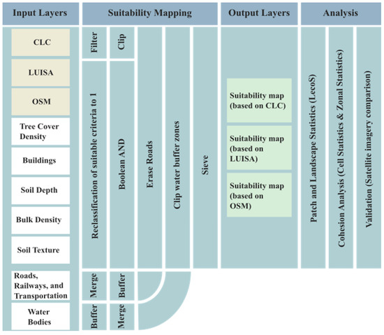
Figure 2.
The GIS-based workflow of this test study.
The GIS-based approach of this study included, firstly, the selection of open-source input layers at the European scale (Section 3.1), and secondly, the multi-criteria suitability mapping utilising the selected raster and vector input layers (Section 3.2). The suitability mapping was performed by applying the Boolean multi-criteria analysis [40] to three different LULC input layers (CORINE Land Cover, LUISA base map, and OpenStreetMap), which differ in their spatial resolution. The suitability mapping resulted in three outputs (one for each LULC input layer). To gain a better understanding of the impact of the three different spatial resolution layers on the output suitability maps, the following analysis and validation methods were used in the final step (Section 3.3): patch and landscape statistics, cohesion analysis, and satellite validation.
3.1. Input Layers
At the European scale, the following three possible LULC input layers (which provide a sufficient classification of land cover types) were identified with differing spatial resolutions:
- CORINE Land Cover (CLC) [41], published in 2018, presents a visual interpretation of high-resolution satellite imagery from 2017 and 2018. The raster layer has a spatial resolution of a minimum of 100 m, a data storage size of 206.2 MB, and contains 44 LULC classes.
- LUISA base map (2018) [42] builds on the CLC layer (2018), COPERNICUS high-resolution (10 m) layers from 2018, the COPERNICUS Urban Atlas (2018), the Global Human Settlement Layer (2015), the TomTom Multinet vector layer, and OpenStreetMap data (2020). The LUISA base map is a raster layer with a minimum spatial resolution of 50 m and a data storage size of 1.02 GB.
- OpenStreetMap (OSM) [43] is a crowdsourced vector layer produced and updated by volunteers digitising satellite imagery, and it is validated with aerial imagery, GPS devices, and low-tech field maps. The dataset has an accuracy of at best 2 m, and a data storage size of 26 GB for Europe in 2022.
For the other identified suitability criteria in (Section 2), representative open-source datasets at the European scale were selected for the suitability mapping. The representative datasets, along with the related suitability criteria, their spatial resolution, temporal range, and source, are listed in Table 1.

Table 1.
Input layers for the suitability mapping of riparian forest buffers.
Resampling and reprojection. As all selected layers differ in their spatial resolution (see Table 1) and the suitability mapping works on cell level, the input layers were resampled to one common spatial resolution of 10 m. Discrete layers (soil texture and buildings) were resampled by applying the nearest neighbour method; whereas, layers with more continuous information (tree cover density, soil depth, and bulk density) were resampled using the cubic method. In addition, all layers were reprojected to the following common coordinate reference system: the ETRS89 Lambert Azimuthal Equal-Area projection coordinate reference system (EPSG:3035).
3.2. Suitability Mapping Based on Multi-Criteria Analysis
The method of multi-criteria analysis (MCA) offers the possibility to integrate a larger number of criteria that need to be considered for assessing the suitability of an area. As introduced above, NBS are selected based on different suitability criteria. MCA enables the integration of all criteria. Similar to the method used by other NBS decision tools [5,7,11,12], for the MCA suitability mapping, the layers for each criterion are overlaid to identify areas where all criteria are met. GIS-based MCA methods offer three ways for overlaying layers [40], as follows: (1) Boolean; (2) weighted; or (3) fuzzy memberships. For this study, the Boolean method was chosen to be most suitable, and was used in this study.
Creation Boolean layers. For the MCA, all input layers were transformed into Boolean layers. In particular, the CLC and LUISA land cover layers, as well as additional raster layers (soil depth, bulk density, soil texture, tree cover density, and buildings), were reclassified (according to the criteria outlined in Table 1) to a binary scale with values of 0 and 1, of which the value of 1 indicates suitable areas. For the OSM vector layer, suitable land covers were filtered and extracted. Intermediate results are presented as follows in Figure 3, which displays the suitable areas indicated by the three LULC layers: Figure 3a (LUISA), Figure 3b (OSM), and Figure 3c (CLC).
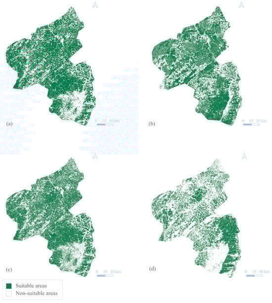
Figure 3.
This figure presents the Boolean output layers for the study state of Rhineland Palatinate in Germany; (a–c) present each of the three LULC layers after the reclassification to Boolean layers: (a) LUISA base map, (b) OSM, (c) CLC; and (d) presents the suitable areas where all criteria (except LULC) are indicating suitability.
Boolean multi-criteria analysis. The first part of the MCA was performed with the Boolean AND tool. This intermediate output layer (Figure 3d) shows all suitable areas where all criteria are met (except LULC layers). Following this step, the intermediate layer was overlayed with each of the three binary LULC layers. To include vector layers in the Boolean MCA, a different approach was adopted, since the Boolean AND is a raster tool. Hence, the filtered OSM layer was used to extract suitable areas. After this process, three output suitability maps were available, one for each of the three LULC layers. To further exclude transport lines, the OSM line vector layers of roads, railways, and transport were merged and buffered with 3 m. With this resulting layer, suitable areas located on these transportation lines could be removed with the erase tool. Similarly, the EU-Hydro layers were merged and buffered with different buffer widths depending on the type of waterway (see Table 1). Finally, suitable areas within the water buffer could be extracted.
Exclusion of fragmented areas. The three resulting output layers show suitable areas along rivers, streams, ditches, and canals. However, these areas were found to be highly fragmented, considering that riparian forest buffers are more effective when they are, firstly, connected to existing forest habitats, and secondly, when they have minimum lengths and widths. Therefore, the three outputs were further processed to exclude small areas. This exclusion of areas less than 100 aligned cells (with a 10 m resolution) was performed with the GDAL sieve tool, and the final suitability maps were produced.
3.3. Analysis and Validation
The suitability mapping resulted in three different outputs. Based on these, further analysis and validation was performed to gain a better understanding on the suitability of each LULC layer for the integration into Europe-wide suitability mapping for the NBS Toolkit. For this purpose, the three output suitability layers were quantitatively analysed with cell and patch statistics, and qualitatively validated with satellite imagery.
Cell statistics. QGIS raster cells statistics were applied to assess the coherence of the three output layers. Comparing these layers on a cell-basis indicates whether the outputs suggest the same suitable areas or not. In particular, a new layer was created in which each cell has a value ranging from 0–3:3, indicating high coherence—meaning that all three suitability mapping outputs suggest suitability; a value of 2 presents areas where two layers (out of the three) indicate suitability, 1 suitability is suggested with one layer only, and those with a value of 0 are non-suitable areas.
Patch statistics. Statistical analysis, or so-called patch statistics, was used to derive information on the suggested riparian forest buffer sizes and the degree of fragmentation. Patch statistics were performed using the QGIS plugin LecoS 3.0 [48]. This plugin is based on the FRAGSTATS (v4) software [49] commonly used in landscape ecology for patch and landscape analysis. The following metrices were calculated: (1) land cover, to calculate the entire area for potential riparian forest buffers; (2) number of patches, to present the difference in the number of suggested areas; (3) patch density (land cover divided by number of patches), which indicates how dense the suggested riparian forests are to each other; (4) maximum and mean riparian area sizes; and (5) the landscape division index, to analyse the degree of fragmentation of the suggested riparian forest areas with values ranging between 0 and 1, while 1 indicates patchiness, and hence, fragmentation.
Satellite image validation. Qualitative assessment was used to validate the (thematic) accuracy and appropriateness of the suggested riparian areas. At this point, we define thematic accuracy as the correctness degree of the suggested areas; for instance, considering a LULC layer of 100 m, the resolution cannot present LULC class borders as accurate as in reality, whilst the appropriateness is considered as the actual suitability of a suggested area. For this qualitative validation, the Google satellite images layer (2022) was overlayed with each of the three output maps to assess whether suggested areas are thematically accurate and appropriate. For instance, whether suitable areas are placed inside water areas (due to a lack of accuracy) or on camping sites (which may not be appropriate).
4. Results
The suitability mapping resulted in three different suitability maps (one for each LULC input layer), indicating areas suitable for implementing riparian forest buffer zones. These three suitability maps were further analysed with (1) cell statistics to compare the suggested suitable areas in terms of coherence with another; (2) patch statistics to assess the degree of fragmentation of proposed suitable areas; and (3) satellite image validation to qualitatively assess the accuracy and appropriateness of the suggested areas. The results of these analyses are presented in the following section.
Suitable area size comparison. Overall, the three maps differ in the total size of suitable area and their structure (e.g., number of suitable areas; maximum and mean size). The total size of suitable areas (Table 2) for the LUISA- and CLC-based output maps is around 25,000,000 m2, while the OSM-based suitability map differs greatly by counting only 14,381,000 m2. According to the results listed in Table 2, the largest and the mean suggested areas (patches) are of a similar size between all output layers. Interestingly, the sizes of the largest patch and of the mean patch area are higher before removing (sieving) small areas.
Table 2.
Patch statistics of the suitability mapping output layers for each LULC input layer before and after removing isolated small areas (sieving).
Suitable area coherence. Comparing the actual suggested areas by overlaying these three output layers and using cell statistics (Figure 4), only 56.8% of the suggested areas are found to be coherent between all three layers, 31.6% by two layers, and 10.6% by single layers. Hence, the results show that the output maps greatly differ from one another, while the difference of 11.2% between the outputs of the CLC and LUISA layers is much lower than that of the OSM layer. This result can be explained by the fact that the LUISA layer is based on the CLC layer.
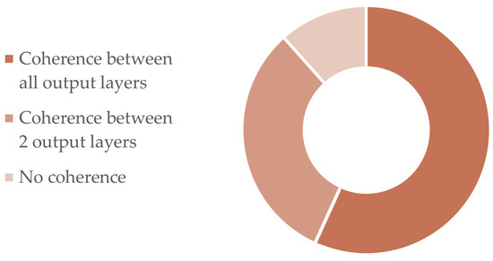
Figure 4.
Coherence between suitability mapping output layers based on CLC, LUISA, and OSM.
Fragmentation. The statistical analysis was used to derive an understanding of the degree of fragmentation. As described in Section 3.2, smaller isolated areas were excluded with the sieving function. The patch statistic results (Table 2) show that through the sieving process, the number of patches of the OSM-based suitability map decreased drastically (compared to the other two outputs). The extensive removal of smaller areas can imply a prior greater degree of fragmentation, which was further explored with the landscape division index and may be explained by the fine spatial resolution. The results show that all output layers have a value close to 1, presenting a great fragmentation which can be traced back to the fact that suitable areas are only located along water areas. However, the index numbers show a minor improvement in fragmentation after the removal of smaller areas. Overall, the OSM-based output has a slightly smaller fragmentation rate than the other two layers.
Thematic accuracy and appropriateness. The satellite image validation method highlighted a few differences and similarities between the suitability maps of each of the three layers. Firstly, the fine resolution input layer OSM could include non-built areas close to urban areas as suitable spots, while these spaces can be classified as urban areas for the CLC and LUISA maps (see Figure 5a). Secondly, some suitable areas highlighted the inaccuracy due to the coarser resolution of the CLC layer. Figure 5b presents one example of this inaccuracy, where suitable areas are suggested on vineyards and a road, which were defined as non-suitable criteria and should, therefore, be excluded. Thirdly, it was found that inaccuracy of input layers (e.g., displaced ditches) is carried along to the output suitability map (Figure 5c). Overall, the three output layers showed greater coherence in agricultural areas (exemplified in Figure 5d). In comparison to non-sieved output layers, the sieved output layers show less suggestions along larger rivers, such as the Rhine. Whilst some suggested areas are located along the Moselle, no suitable areas were detected along the river Ahr, which can be reasoned by the high coverage of already existing riparian vegetation buffering the river. A general coherence between the output files was spotted in agricultural landscapes, which are, at the same time, more homogeneous areas than urban areas.
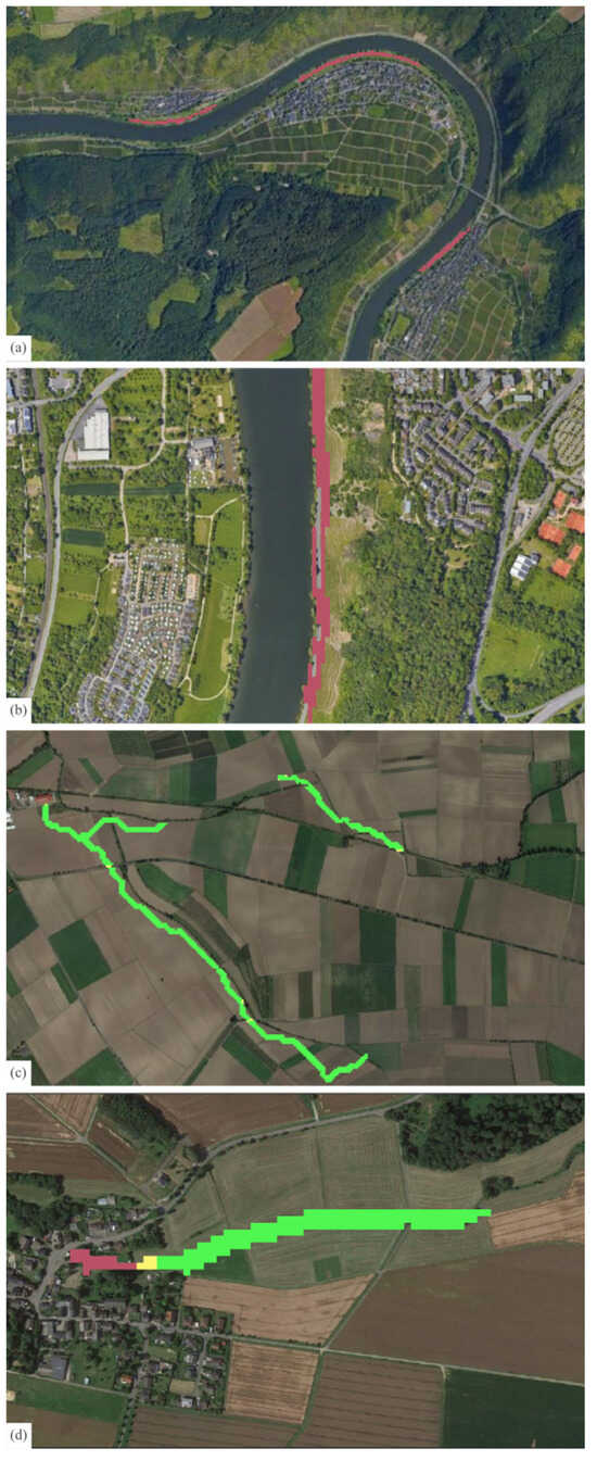
Figure 5.
Results from satellite imagery validation: (a) red marked areas presenting potential riparian forest buffers suggested by the OSM-based suitability map, but not by the other two outputs (coordinates: 4120537 3005590: 4124094 3007762); (b) red areas present non-appropriate suggested areas by the CLC-based suitability map, but not by the other two outputs (coordinates: 4146529 3027011: 4147856 3027821); (c) inaccuracy of input and output layers (coordinates: 4191466 2963021: 4194514 2964882); (d) the general agreement of all output layers is marked in green, while yellow presents the agreement of two layers, and red is only one layer (coordinates: 4162673 3014443: 4163541 3014973).
Data storage size and processing time. The data storage size of the three LULC layers varies greatly (ranging from 206.2 MB to 26 GB) for the entirety of Europe, depending on their resolution. However, the suitability output maps are of the same size. For the study area, no considerable differences in processing times were detected, perhaps because the area is rather small (compared to the European region). Nonetheless, the input data storage size is expected to have an impact on the computation time for the entirety of Europe.
5. Discussion
In this study, we tested the impact of different spatial resolutions on the output of the suitability mapping to support our decision of a suitable input LULC layer for the suitability mapping of the NBS Toolkit.
Overall, the results showed a great sensitivity when comparing the suitability maps of different resolution LULC input layers. This was indicated by the different analyses. Firstly, the cell statistics showed that the suitability mapping outputs of coarser resolution layers were more coherent with another than with the fine resolution layer. Secondly, a high sensitivity was detected through the patch statistics in the total size of suggested areas, the number of patches, the degree of fragmentation, and in the coherence analysis of all layers. Thirdly, the qualitative accuracy and appropriateness validation results suggest that the OSM fine resolution layer was more accurate and appropriate than the coarsest layer, especially close to low-density urban areas or houses. This finding aligns with the outcomes of Grafius et al. [19], stating that fine resolution layers are recommended to be used for urban analysis. However, in this study, rural areas were the focus and, therefore, the fine resolution layer showed only minor advantages compared to the coarser layers, based on the satellite imagery validation. In more homogenous land covers and uses (e.g., agricultural land), the coherence between all layers was greatest; thus, for these areas, the usage of coarser resolution layers can be sufficient, considering higher computational processing time of fine resolution layers, but also increasing processing complexity due to working with different data types (e.g., raster and vector). Lastly, the computation showed that there are no major differences in processing time within the study area, but it can be assumed that for computation at the European scale, a difference will become obvious [15].
It can be concluded that the findings confirm the hypothesis that the resolution of LULC input datasets for suitability mapping needs to be determined in alignment with the aimed landscape type (urban or rural), as coarser resolution layers with, e.g., 100 m resolutions may not be accurate enough for highly heterogenous urban landscapes. Furthermore, which Nature-Based Solution the suitability mapping is focusing on needs to be considered. In this study, a large-scale NBS was selected, but for small-scale NBS, such as ponds and basins, finer resolution layers can be more appropriate. Hence, for decision-making on input layer’s spatial resolution for suitable mapping, the desired goal (NBS scale and landscape) needs to be taken into account. This conclusion reflects findings in other studies [18,19].
Even though the suitability of data for an intended purpose may not always be defined based on statistical measures [50], we used the results of this study to support our decision-making on the most suitable input layer for the computation of suitability maps for Europe. Based on the results, we utilise the LUISA layer for assessing the suitability of riparian forest buffers across Europe. However, for small-scale Nature-Based Solutions, or for solutions to be implemented in (semi-)urban areas, the toolkit will be using the OSM fine resolution layer.
Finally, it can be recapped that the suitability mapping at the European scale functions as a pre-assessment and, therefore, inaccuracy in mapping may be caused by the coarseness of the input datasets. As we have seen, even the fine resolution layer indicated inaccuracies which could not be prevented. Hence, we argue that a local and context-specific assessment (including, i.e., social, economic, and political criteria) is necessary for in-depth validation and for final decision-making to avoid implications for the environment, society, and overall flood risk [3,51,52,53].
6. Conclusions
This study was performed to support the development of an innovative toolkit for decision-support on Nature-Based Solutions across Europe. The NBS Toolkit is based on open-source datasets. For many of the NBS suitability criteria, there is only one dataset available at the European scale, but for the land use and land cover, several datasets are openly available at different spatial resolutions. Several studies in other research fields are discussing the influence of spatial resolution on the outcome, but this was not tested in context of the suitability mapping of Nature-Based Solutions. To gain a better understanding on the impact of the resolution on the final NBS suitability map, this study compares the outcomes of three European land use and land cover layers to different spatial resolutions in a test area in Germany. The results of this study suggest that for rural areas and larger scale NBS, coarser input layers can be sufficient, while for urban and small-scale NBS, finer resolution may be required. These results were integrated into the development of the NBS Toolkit and, therefore, the suitability mapping method could be upscaled to Europe. Furthermore, the method will be replicated in other regions, such as in Africa. Overall, this study extended the existing scholarship for NBS suitability mapping.
Author Contributions
Conceptualisation, J.O., J.N. and M.K.; methodology, J.O.; software, J.O., J.N. and S.V.; validation, J.O., M.K., J.N. and H.L.C.; formal analysis, J.O.; data curation, J.O.; writing—original draft preparation, J.O.; writing—review and editing, J.O., J.N., S.V., M.K. and H.L.C.; visualisation, J.O.; supervision, J.N., S.V., M.K., L.S.L., S.D.S. and H.L.C.; project administration, L.S.L. and S.D.S.; funding acquisition, S.D.S. All authors have read and agreed to the published version of the manuscript.
Funding
This work was funded by and carried out within the framework of the OPERANDUM project supported by the European Union’s (EU) Horizon2020 research and innovation program (Grant No. 776848), and the ALBATROSS project supported by the European Union (G.A. No. 101137895). J. Neumann and H. L. Cloke were supported by the LANDWISE project funded by the Natural Environment Research Council (NERC) (Grant No. NE/R004668/1).
Data Availability Statement
The data that support the findings of this study are available from the corresponding author upon reasonable request. In case of a request, the authors will provide a citation along with the requested dataset.
Conflicts of Interest
Authors Joy Ommer, Saša Vranić and Milan Kalas were employed by the company KAJO s.r.o. The remaining authors declare that the research was conducted in the absence of any commercial or financial relationships that could be construed as a potential conflict of interest.
References
- Debele, S.E.; Leo, L.S.; Kumar, P.; Sahani, J.; Ommer, J.; Bucchignani, E.; Vranić, S.; Kalas, M.; Amirzada, Z.; Pavlova, I.; et al. Nature-Based Solutions Can Help Reduce the Impact of Natural Hazards: A Global Analysis of NBS Case Studies. Sci. Total Environ. 2023, 902, 165824. [Google Scholar] [CrossRef]
- Cohen-Shacham, E.; Walters, G.; Janzen, C.; Maginnis, S. Nature-Based Solutions to Address Global Societal Challenges; IUCN International Union for Conservation of Nature: Gland, Switzerland, 2016. [Google Scholar]
- Ommer, J.; Bucchignani, E.; Leo, L.S.; Kalas, M.; Vranić, S.; Debele, S.; Kumar, P.; Cloke, H.L.; Di Sabatino, S. Quantifying Co-Benefits and Disbenefits of Nature-Based Solutions Targeting Disaster Risk Reduction. Int. J. Disaster Risk Reduct. 2022, 75, 102966. [Google Scholar] [CrossRef]
- Amirzada, Z.; Pavlova, I.; de Chaisemartin, M.; Denoon, R.; Kalas, M.; Vranić, S.; Ommer, J.; Sabbatini, T.; Kumar, P.; Debele, S.; et al. Reducing Hydro-Meteorological Risks through Nature-Based Solutions: A Comprehensive Review of Enabling Policy Frameworks in the European Union. Nat.-Based Solut. 2023, 4, 100097. [Google Scholar] [CrossRef]
- Mubeen, A.; Ruangpan, L.; Vojinovic, Z.; Sanchez Torrez, A.; Plavšić, J. Planning and Suitability Assessment of Large-Scale Nature-Based Solutions for Flood-Risk Reduction. Water Resour. Manag. 2021, 35, 3063–3081. [Google Scholar] [CrossRef]
- Sarabi, S.; Han, Q.; de Vries, B.; Romme, A.G.L. The Nature-Based Solutions Planning Support System: A Playground for Site and Solution Prioritization. Sustain. Cities Soc. 2022, 78, 103608. [Google Scholar] [CrossRef]
- PEDRR Opportunity Mapping. Available online: https://pedrr.org/mapping-eco-drr-opportunities/ (accessed on 23 April 2024).
- Croeser, T.; Garrard, G.; Sharma, R.; Ossola, A.; Bekessy, S. Choosing the Right Nature-Based Solutions to Meet Diverse Urban Challenges. Urban Urban Green 2021, 65, 127337. [Google Scholar] [CrossRef]
- Anderson, C.C.; Renaud, F.G. A Review of Public Acceptance of Nature-Based Solutions: The ‘Why’, ‘When’, and ‘How’ of Success for Disaster Risk Reduction Measures. Ambio 2021, 50, 1552–1573. [Google Scholar] [CrossRef]
- Giordano, R.; Pluchinotta, I.; Pagano, A.; Scrieciu, A.; Nanu, F. Enhancing Nature-Based Solutions Acceptance through Stakeholders’ Engagement in Co-Benefits Identification and Trade-Offs Analysis. Sci. Total Environ. 2020, 713, 136552. [Google Scholar] [CrossRef]
- Kuller, M.; Bach, P.M.; Roberts, S.; Browne, D.; Deletic, A. A Planning-Support Tool for Spatial Suitability Assessment of Green Urban Stormwater Infrastructure. Sci. Total Environ. 2019, 686, 856–868. [Google Scholar] [CrossRef]
- Guerrero, P.; Haase, D.; Albert, C. Locating Spatial Opportunities for Nature-Based Solutions: A River Landscape Application. Water 2018, 10, 1869. [Google Scholar] [CrossRef]
- OPERANDUM GeoIKP: NBS Toolkit. Available online: https://geoikp.operandum-project.eu/nbs/toolkit (accessed on 23 April 2024).
- Chen, W.; Li, D.-H.; Yang, K.-J.; Tsai, F.; Seeboonruang, U. Identifying and Comparing Relatively High Soil Erosion Sites with Four DEMs. Ecol. Eng. 2018, 120, 449–463. [Google Scholar] [CrossRef]
- Buakhao, W.; Kangrang, A. DEM Resolution Impact on the Estimation of the Physical Characteristics of Watersheds by Using SWAT. Adv. Civ. Eng. 2016, 2016, 8180158. [Google Scholar] [CrossRef]
- Avand, M.; Kuriqi, A.; Khazaei, M.; Ghorbanzadeh, O. DEM Resolution Effects on Machine Learning Performance for Flood Probability Mapping. J. Hydro-Environ. Res. 2022, 40, 1–16. [Google Scholar] [CrossRef]
- Dixon, B.; Earls, J. Resample or Not?! Effects of Resolution of DEMs in Watershed Modeling. Hydrol. Process. 2009, 23, 1714–1724. [Google Scholar] [CrossRef]
- Nazari-Sharabian, M.; Taheriyoun, M.; Karakouzian, M. Sensitivity Analysis of the DEM Resolution and Effective Parameters of Runoff Yield in the SWAT Model: A Case Study. J. Water Supply: Res. Technol. Aqua 2020, 69, 39–54. [Google Scholar] [CrossRef]
- Grafius, D.R.; Corstanje, R.; Warren, P.H.; Evans, K.L.; Hancock, S.; Harris, J.A. The Impact of Land Use/Land Cover Scale on Modelling Urban Ecosystem Services. Landsc. Ecol. 2016, 31, 1509–1522. [Google Scholar] [CrossRef]
- Di Sabatino, A.; Coscieme, L.; Vignini, P.; Cicolani, B. Scale and Ecological Dependence of Ecosystem Services Evaluation: Spatial Extension and Economic Value of Freshwater Ecosystems in Italy. Ecol. Indic. 2013, 32, 259–263. [Google Scholar] [CrossRef]
- Peter, B.G.; Messina, J.P.; Lin, Z.; Snapp, S.S. Crop Climate Suitability Mapping on the Cloud: A Geovisualization Application for Sustainable Agriculture. Sci. Rep. 2020, 10, 15487. [Google Scholar] [CrossRef]
- Birkmann, J.; Schüttrumpf, H.; Handmer, J.; Thieken, A.; Kuhlicke, C.; Truedinger, A.; Sauter, H.; Klopries, E.-M.; Greiving, S.; Jamshed, A.; et al. Strengthening Resilience in Reconstruction after Extreme Events—Insights from Flood Affected Communities in Germany. Int. J. Disaster Risk Reduct. 2023, 96, 103965. [Google Scholar] [CrossRef]
- Koks, E.E.; van Ginkel, K.C.H.; van Marle, M.J.E.; Lemnitzer, A. Brief Communication: Critical Infrastructure Impacts of the 2021 Mid-July Western European Flood Event. Nat. Hazards Earth Syst. Sci. 2022, 22, 3831–3838. [Google Scholar] [CrossRef]
- Fekete, A.; Sandholz, S. Here Comes the Flood, but Not Failure? Lessons to Learn after the Heavy Rain and Pluvial Floods in Germany 2021. Water 2021, 13, 3016. [Google Scholar] [CrossRef]
- Graziano, M.P.; Deguire, A.K.; Surasinghe, T.D. Riparian Buffers as a Critical Landscape Feature: Insights for Riverscape Conservation and Policy Renovations. Diversity 2022, 14, 172. [Google Scholar] [CrossRef]
- Broadmeadow, S.; Nisbet, T.R. The Effects of Riparian Forest Management on the Freshwater Environment: A Literature Review of Best Management Practice. Hydrol. Earth Syst. Sci. 2004, 8, 286–305. [Google Scholar] [CrossRef]
- Weissteiner, C.; Ickerott, M.; Ott, H.; Probeck, M.; Ramminger, G.; Clerici, N.; Dufourmont, H.; de Sousa, A. Europe’s Green Arteries—A Continental Dataset of Riparian Zones. Remote Sens. 2016, 8, 925. [Google Scholar] [CrossRef]
- Yirigui, Y.; Lee, S.-W.; Nejadhashemi, A.P.; Herman, M.R.; Lee, J.-W. Relationships between Riparian Forest Fragmentation and Biological Indicators of Streams. Sustainability 2019, 11, 2870. [Google Scholar] [CrossRef]
- Liu, J.; Wilson, M.; Hu, G.; Liu, J.; Wu, J.; Yu, M. How Does Habitat Fragmentation Affect the Biodiversity and Ecosystem Functioning Relationship? Landsc. Ecol. 2018, 33, 341–352. [Google Scholar] [CrossRef]
- European Union; Copernicus Land Monitoring Service. EU-Hydro; European Environment Agency: Copenhagen, Denmark, 2020. [Google Scholar]
- Dottori, F.; Alfieri, L.; Bianchi, A.; Skoien, J.; Salamon, P. River Flood Hazard Maps for Europe and the Mediterranean Basin Region; European Commission: Ispra, Italy, 2021. [Google Scholar]
- Addy, S.; Wilkinson, M. The Bowmont Catchment Initiative: An Assessment of Catchment Hydrology and Natural Flood Management Measures; Scottish Government: Edinburgh, UK, 2017. [Google Scholar]
- Jerrentrup, H.; Efthimiou, G. Results of Riparian Forest Restoration in Nestos Delta, NE-Greece 10 Years after Plantation. In Proceedings of the European River Restoration Conference, Vienna, Austria, 11–13 September 2013; p. 1. [Google Scholar]
- EEA. Water-Retention Potential of Europe’s Forests: A European Overview to Support Natural Water-Retention Measures; European Environment Agency: Luxembourg, 2015. [Google Scholar]
- Schenk, H.J.; Jackson, R.B. Rooting Depths, Lateral Root Spreads and Below-ground/Above-ground Allometries of Plants in Water-limited Ecosystems. J. Ecol. 2002, 90, 480–494. [Google Scholar] [CrossRef]
- Grant, R.F. Simulation Model of Soil Compaction and Root Growth: II. Model Performance and Validation. Plant Soil 1993, 150, 15–24. [Google Scholar] [CrossRef]
- Kumar, A.; Verma, P.; Sharma, M.K. Irrigation Management in Stone Fruits. In Production Technology of Stone Fruits; Springer: Singapore, 2021; pp. 171–187. [Google Scholar]
- Richardson, J.S.; Naiman, R.J.; Bisson, P.A. How Did Fixed-Width Buffers Become Standard Practice for Protecting Freshwaters and Their Riparian Areas from Forest Harvest Practices? Freshw. Sci. 2012, 31, 232–238. [Google Scholar] [CrossRef]
- Ngo, T.; Yoo, D.; Lee, Y.; Kim, J. Optimization of Upstream Detention Reservoir Facilities for Downstream Flood Mitigation in Urban Areas. Water 2016, 8, 290. [Google Scholar] [CrossRef]
- Eastman, J.R. Multi-Criteria Evaluation and GIS. In Geographical Information Systems; Goodchild, M.F., Maguire, D.J., Rhind, D.W., Eds.; Longley, John Wiley and Sons: New York, NY, USA, 1999; pp. 493–502. [Google Scholar]
- European Union; Copernicus Land Monitoring Service. Corine Land Cover (CLC) 2018, Version 2020_20u1; European Environment Agency: Copenhagen, Denmark, 2020. [Google Scholar]
- Batista, F.; Pigaiani, C. LUISA Base Map 2018; European Commission: Ispra, Italy, 2021. [Google Scholar]
- OpenStreetMap Germany [Dataset]; 2022.
- European Union; Copernicus Land Monitoring Service. Tree Cover Density 2018; European Environment Agency: Copenhagen, Denmark, 2018. [Google Scholar]
- Corbane, C.; Sabo, F. ESM R2019—European Settlement Map from Copernicus Very High Resolution Data for Reference Year 2015; European Commission: Ispra, Italy, 2019. [Google Scholar]
- ISRIC World Soil Information. SoilGrids250m 2017-03—Absolute Depth to Bedrock; ISRIC: Wageningen, The Netherlands, 2017. [Google Scholar]
- Ballabio, C.; Panagos, P.; Montanarella, L. Mapping Topsoil Physical Properties at European Scale Using the LUCAS Database. Geoderma 2016, 261, 110–123. [Google Scholar] [CrossRef]
- Jung, M. LecoS—A QGIS Plugin for Automated Landscape Ecology Analysis. PeerJ 2013, 31, 18–21. [Google Scholar] [CrossRef][Green Version]
- McGarigal, K.; Marks, B.J. FRAGSTATS: Spatial Pattern Analysis Program for Quantifying Landscape Structure; US Department of Agriculture, Pacific Northwest Research Station: Portland, OR, USA, 1995. [Google Scholar]
- Leyk, S.; Gaughan, A.E.; Adamo, S.B.; de Sherbinin, A.; Balk, D.; Freire, S.; Rose, A.; Stevens, F.R.; Blankespoor, B.; Frye, C.; et al. The Spatial Allocation of Population: A Review of Large-Scale Gridded Population Data Products and Their Fitness for Use. Earth Syst. Sci. Data 2019, 11, 1385–1409. [Google Scholar] [CrossRef]
- Sarker, S. Separation of Floodplain Flow and Bankfull Discharge: Application of 1D Momentum Equation Solver and MIKE 21C. CivilEng 2023, 4, 933–948. [Google Scholar] [CrossRef]
- European Commission. Evaluating the Impact of Nature-Based Solutions: A Handbook for Practitioners; Publications Office of the European Union: Luxembourg, 2021. [Google Scholar]
- Gonzalez-Ollauri, A.; Mickovski, S.B.; Anderson, C.C.; Debele, S.; Emmanuel, R.; Kumar, P.; Loupis, M.; Ommer, J.; Pfeiffer, J.; Panga, D.; et al. A Nature-Based Solution Selection Framework: Criteria and Processes for Addressing Hydro-Meteorological Hazards at Open-Air Laboratories across Europe. J. Environ. Manag. 2023, 331, 117183. [Google Scholar] [CrossRef]


Disclaimer/Publisher’s Note: The statements, opinions and data contained in all publications are solely those of the individual author(s) and contributor(s) and not of MDPI and/or the editor(s). MDPI and/or the editor(s) disclaim responsibility for any injury to people or property resulting from any ideas, methods, instructions or products referred to in the content. |
© 2024 by the authors. Licensee MDPI, Basel, Switzerland. This article is an open access article distributed under the terms and conditions of the Creative Commons Attribution (CC BY) license (https://creativecommons.org/licenses/by/4.0/).