Improvement of Blocked Long-Straight Flow Channels in Proton Exchange Membrane Fuel Cells Using CFD Modeling, Artificial Neural Network, and Genetic Algorithm

Abstract

To further improve the performance of the Proton Exchange Membrane Fuel Cell (PEMFC), in this paper, we designed a blocked flow channel with trapezoidal baffles, and geometric parameters of the baffle were optimized based on CFD simulation, Artificial Neural Network (ANN), and single-objective optimization methods. The analysis of velocity, pressure, and oxygen distribution in the cathode flow channel shows that the optimized trapezoidal baffle can improve oxygen transport during the reaction. The comparison of the optimization model with the straight flow channel model and the rectangular baffle model shows that the power density of the optimized model is 4.0% higher than that of the straight flow channel model at a voltage of 0.3 V, and the pressure drop is only 37.83% of that of the rectangular baffle model. For on-road PEMFC with a voltage of 0.6 V, the influence of pump power is significant, and the optimized trapezoidal baffle model has a net power increase of 1.47% compared to the rectangular baffle model at 50% pump efficiency and 3.94% at 30% pump efficiency.

1. Introduction

The Proton Exchange Membrane Fuel Cell (PEMFC) shows promising advantages for its high efficiency and zero emission compared with internal combustion engines [1,2]. The membrane would show low resistance with ample water inside, which means the reactive gases need humidification. The area with a relatively high electrochemical reaction rate has a higher risk of flooding because the product of the reaction is also water [3,4]. The operating temperature range of PEMFC is determined by the physicochemical properties of the membrane [5]. Therefore, heat and water management is crucial to PEMFC [5,6]. The mass transport of reactive gases is also essential to the performance and reliability of PEMFC. The uniform distribution of reactive gases helps reduce the risk of high temperatures and flooding in local areas in the flow field [7,8,9].

There are several researches about the mass transport in PEMFC. Hakenjos et al. designed and tested a visible single PEMFC, measured the distribution of current density and temperature, and studied the shape and movement of water drops in the flow channel [10]. Nandjou et al. conducted a durability test and researched the degradation mechanisms of the components in PEMFC by many measuring means [11]. Sakaida et al. established the gas diffusion layer (GDL) structure by X-ray measurements and researched the movement of water drops in the GDL by the lattice Boltzmann method (LBM) [12]. Shao et al. studied the hysteresis of output voltage by a visualization experiment and Electrochemical Impedance Spectroscopy (EIS), built a 1-D PEMFC model to calculate, and indicated the importance of GDL wettability to liquid water transport [13]. Shao et al. built a 2-D PEMFC model to research the effect of water transport in the cathode on the performance of PEMFC [14]. Zhao et al. studied the O₂ transport in the membrane electrode assembly (MEA) by calculation and experiment [15]. Peng et al. studied the effect of the accumulation of water and N₂ in anode on the performance by a 3-D transient calculation [16].

Some research focuses on the influence of flow field structure on the performance of PEMFC. Peng et al. modeled the fuel cell and researched the influence of different flow field structures on the temperature distribution of commercial PEMFC [17]. Li et al. simulated the cathode variable cross-section flow channel model to improve the performance of PEMFC [18]. Luo et al. designed and calculated a serpentine flow field with rib grooves to optimize the performance of PEMFC [19]. Saripella et al. researched the influence of bio-inspired flow channels on the performance of PEMFC by simulation and experiment [20]. Zamora-Antuñano et al. made a CFD model of a PEMFC and analyzed the influence of channel distribution on the cathode current [21]. Each flow field design has certain disadvantages. The parallel flow field shows worse distribution uniformity of reactive gases than the serpentine and the interdigital flow fields [22]. Methods in former research to improve the distribution uniformity of reactive gases, namely changing the cross-section flow channel or adding block structure, or baffles, in the flow channel, have been investigated [23,24,25,26,27]. Zhang et al. built a fuel cell model with baffles in cathode flow channels to study the influence of the distribution and size of baffles on the performance of PEMFC, and found that the baffles in flow channels could improve the performance of PEMFC by enhancing the distribution uniformity of reactive gases [28].

To save time and calculation resources, a series of fuel cell models were designed, and surrogate models were trained by machine learning to optimize the fuel cell performance based on the chosen algorithm [29]. Cao et al. made an Artificial Neural Network (ANN) model to predict the cell voltage consistency of a PEMFC [30]. Qiu et al. made a Radial Basis Function Neural Network (RBFNN) model of PEMFC to optimize the contact pressure of GDL [31]. Yu et al. built a 3-D CFD model of a PEMFC, designed and calculated a series of models, trained a surrogate model by ANN, and optimized the parameters of baffles in the flow channel by Genetic Algorithm (GA) and multi-objective optimization (MOO) to improve the performance of the PEMFC [32].

In this paper, a flow field structure was designed and modified to further improve the performance of the fuel cell with the methods of CFD simulation, ANN, and single-objective optimization. A cathode flow channel model was designed with trapezoidal baffles to increase the oxygen concentration of the catalyst layer (CL), and a CFD simulation model of the PEMFC was established based on the geometric parameters of the flow channel. In the simulation process, to improve the net power output of PEMFC under road conditions, the geometric parameters of the trapezoidal baffle model were optimized using ANN and single-objective optimization methods to improve the overall performance of the on-road PEMFC.

2. Model Development

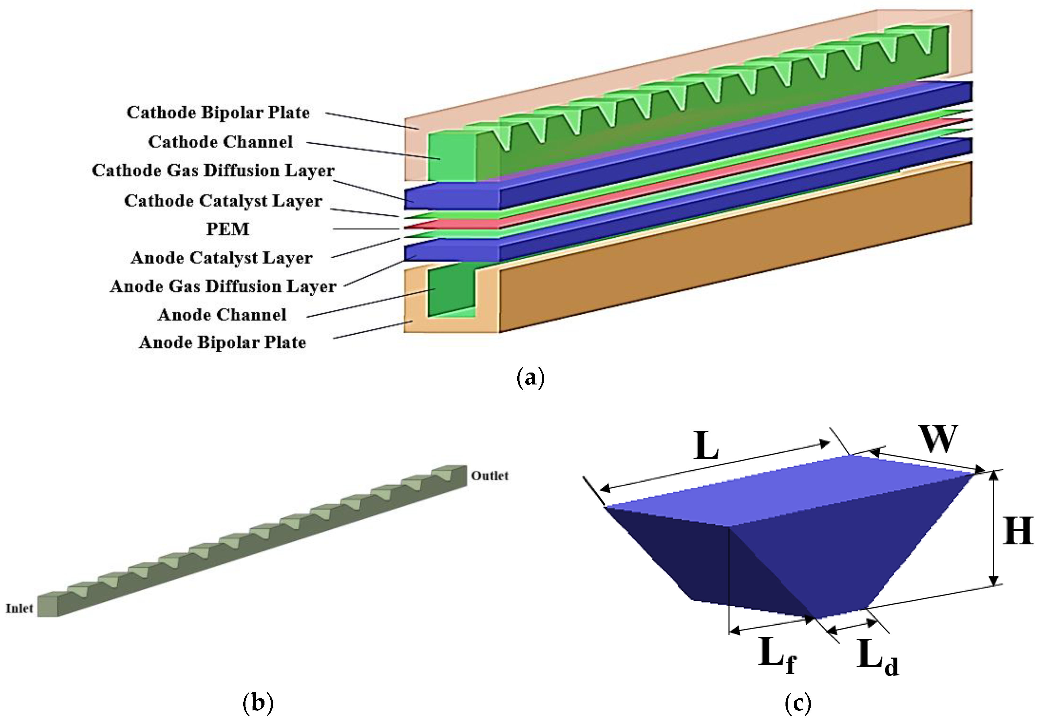
2.1. Geometric Model

The PEMFC model consists of anode and cathode bipolar plates, anode and cathode reaction gas channels, anode and cathode gas diffusion layers, anode and cathode catalytic layers, and proton exchange membranes. The geometrical structure and parameters are shown in Figure 1a and

Table 1. Parameters of geometric model.

Parameters	Values	Unit
Active area	1.2 × 132	mm × mm
Thickness of BP	0.8	mm
Thickness of GDL	0.26	mm
Thickness of CL	0.01	mm
Thickness of membrane	0.03	mm
Depth of flow channel	0.6	mm
Width of flow channel	0.6	mm

. The anode channel is a simple parallel flow field, and the blocked cathode channel applies a series of trapezoidal baffles, as shown in Figure 1b. The reaction gas is affected by the trapezoidal baffles, which disturbs the velocity boundary layer of the flow field. The velocity of the gas flow is increased, and a downward partial velocity is created, which results in forced gas diffusion, increasing the gas concentration near the reaction zone. The trapezoidal baffles’ geometrical structure and parameters are shown in Figure 1c and

Table 2. Parameters of trapezoidal baffles.

Parameters	Values	Unit
Width of baffles (W)	0.6	mm
Length of the upper base (L)	5	mm
Length of the lower base (Ld)	1	mm
Difference between L and Ld (Lf)	2	mm
Attitude of baffles (H)	0.4	mm

, respectively. The lengths of both bases (L and L_d) are constant, and the attitude (H) and the length difference between the two bases towards the inlet (L_f) are selected as the main characteristic parameters of the trapezoidal baffle for the flow field optimization.

2.2. Mathematical Model

A 3-D, multiphase CFD model is built to calculate the flow, mass transport, and electrochemical reaction of the PEMFC. The key physicochemical parameters and governing equations in this model are shown below.

2.2.1. Key Physicochemical Parameters

The key physicochemical parameters in this model are shown in

Table 3. Key physicochemical parameters in this model.

Parameters	Values		Unit
Operation pressure	200,000		Pa
Operation temperature	343.15		K
Output voltage at optimization	0.4		V
Open circuit voltage	1.1		V
Electrical conductivity of BP	1.0 × 106		S/m
Reference concentration	H2: 56.4	O2: 3.39	mol/m3
Stoichiometry ratio	Anode: 1.5	Cathode: 2	-
Porosity of GDL	Anode: 0.4	Cathode: 0.4	-
Porosity of CL	Anode: 0.3	Cathode: 0.3	-
Electrical conductivity of GDL	Anode: 5000	Cathode: 5000	S/m
Relative humidity	Anode: 30%	Cathode: 50%	-
Reference exchange current density	Anode: 13000	Cathode: 30	A/m2
Concentration exponent	Anode: 0.5	Cathode: 1	-

.

2.2.2. Governing Equations

• Mass conservation equation

$$\frac{\partial (\epsilon \rho )}{\partial t}+\nabla \cdot (\epsilon \rho \overrightarrow{u})=S_m,$$

(1)

$$S_{m,a}=S_{H_2}=-\frac{M_{H_2}}{2F}{i}_{an},$$

(2)

$$S_{m,c}=S_{H_{2}O}+S_{O_2}=\frac{M_{H_{2}O}}{2F}{i}_{ca}-\frac{M_{O_2}}{4F}{i}_{ca},$$

(3)

The mass conservation equation is shown in Equation (1). ε is the porosity. ρ is the density of the fluid. S_m is the mass source term, which is zero in reactive gas flow channels and GDL of anode and cathode. S_m,a and S_m,c are the mass source terms in anode and in cathode, as shown in Equations (2) and (3). $M_{H_2}$, $M_{H_{2}O}$, and $M_{O_2}$ are the molar mass of H₂, H₂O, and O₂. F is Faraday constant, 96,485 C/mol. i_an and i_ca are the exchange current densities of anode and cathode.

• Momentum conservation equation

$$\frac{\partial (\epsilon \rho \overrightarrow{u})}{\partial t}+\nabla \cdot (\epsilon \rho \overrightarrow{u}\overrightarrow{u})=-\epsilon \nabla p+\nabla \cdot (\epsilon \mu \nabla \overrightarrow{u})+S_u,$$

(4)

$${\epsilon }_g{u}_g=\frac{k_p}{{\mu }_g}\nabla p_g,$$

(5)

$$S_u=\frac{{\epsilon }_{}^2\mu }{k_p}\overrightarrow{u},$$

(6)

The momentum conservation equation is shown in Equation (4), and S_u is the momentum source term. p is the pressure, and μ is the dynamic viscosity of the fluid.

Equation (4) could be simplified in different components. ε is 1, and S_u is zero in flow channels. Equation (4) is simplified to Equations (5) and (6) in porous medium according to Darcy’s law.

• Energy conservation equation

$$\frac{\partial (\epsilon \rho c_{p}T)}{\partial t}+\nabla \cdot (\epsilon \rho c_p\overrightarrow{u}T)=\nabla \cdot (k^{eff}\nabla T)+S_Q,$$

(7)

$$S_Q=I^2{R}_{ohm}+\beta S_{H_{2}O}{h}_{reaction}+r_w{h}_L+i_{an,ca}\eta ,$$

(8)

The energy conservation equation is shown in Equation (7), and S_Q is the energy source term. c_p is the specific heat at constant pressure. T is the temperature. k^eff is effective thermal conductivity. The calculation of S_Q is shown in Equation (8) considering ohmic heat, chemical reaction heat, phase transition heat, and overpotential. I is the current, and R_ohm is ohmic resistance. β is the ratio of chemical energy and converted heat. $S_{H_{2}O}$ is the rate at which the water vapor is generated. h_reaction is the enthalpy of the electrochemical reaction. r_w is the rate of phase transition of water, and h_L is the enthalpy of phase transition of water. η is overpotential.

• Species conservation equation

$$\frac{\partial (\epsilon c_{an,ca})}{\partial t}+\nabla \cdot (\epsilon \overrightarrow{u}{c}_{an,ca})=\nabla \cdot (D_{an,ca}^{eff}\nabla c_{an,ca})+S_k,$$

(9)

$$S_{H_2}=-\frac{M_{H_2}}{2F}{i}_{an},$$

(10)

$$S_{O_2}=-\frac{M_{O_2}}{4F}{i}_{ca},$$

(11)

$$S_{H_{2}O}=\frac{M_{H_{2}O}}{2F}{i}_{ca},$$

(12)

The species conservation equation is shown in Equation (9), and S_k is the species source term. S_k is zero in the flow channel and in GDL, and can be simplified in CL as shown in Equations (10)–(12). c_an,ca is the constituent concentration, and $D_{an, ca}^{eff}$ is the effective diffusion coefficient of the constituent in anode or in cathode.

• Charge conservation equation

$$\nabla \cdot ({\sigma }_e\nabla {\varphi }_e)+S_e=0,$$

(13)

$$\nabla \cdot ({\sigma }_m\nabla {\varphi }_m)+S_m=0,$$

(14)

$$i_{an}=i_{an,ref}(\frac{C_{H_2}}{C_{H_2,ref}}{)}^{{\gamma }_{an}}(e^{\frac{{\alpha }_{an}F}{RT}{\eta }_{an}}-e^{\frac{{\alpha }_{ca}F}{RT}{\eta }_{ca}}),$$

(15)

$$i_{ca}=i_{ca,ref}(\frac{C_{O_2}}{C_{O_2,ref}}{)}^{{\gamma }_{ca}}(e^{\frac{{\alpha }_{an}F}{RT}{\eta }_{ca}}-e^{\frac{{\alpha }_{ca}F}{RT}{\eta }_{an}}),$$

(16)

$$\eta ={\varphi }_e-{\varphi }_m-V_{oc}^{ref},$$

(17)

The charge conservation equation is shown in Equations (13) and (14). ϕ_ε and ϕ_m represent solid and membrane potential, respectively. S_ε and S_m represent electron and proton current, respectively, and only exist in CL. The values of S_ε and S_m could be calculated by the Butler–Volmer equation, as shown in Equations (15) and (16). And the subscripts of _an and _ca represent anode and cathode, respectively. The relationship between electrode potential, solid potential, and membrane potential is shown as Equation (17).

• Liquid water formation and transport equation [29]

$$\frac{\partial }{\partial t}({\rho }_{l}s)+\nabla \cdot ({\rho }_l{V}_{l}s)=\nabla \cdot \left[{\rho }_l\frac{K{s}^3}{{\mu }_l}\frac{d{p}_c}{ds}\nabla s\right]+r_w,$$

(18)

Important assumptions have been made to solve the equations above.

(1)

Laminar and incompressible flow in flow channels.

(2)

Steady conditions of operating PEMFC.

(3)

Reactive gases as ideal gas.

(4)

Homogeneous porous medium.

(5)

Neglected gravity.

3. Results

3.1. Optimization Process

3.1.1. Numerical Calculation

In this paper, a 3-D multiphase PEMFC model was built with commercial software, ANSYS Fluent 2020 [33]. The coupling equations for pressure and velocity were calculated by the finite volume method of the Semi-Implicit Method for Pressure-Linked Equations (SIMPLE) [34]. The F-cycle in the multigrid cycle was used to improve the convergence and stability of the calculation. The biconjugate gradient stabilized method (BCGSTAB) was used to solve the solid and membrane potential equations. The grid of the model is shown in Figure 2.

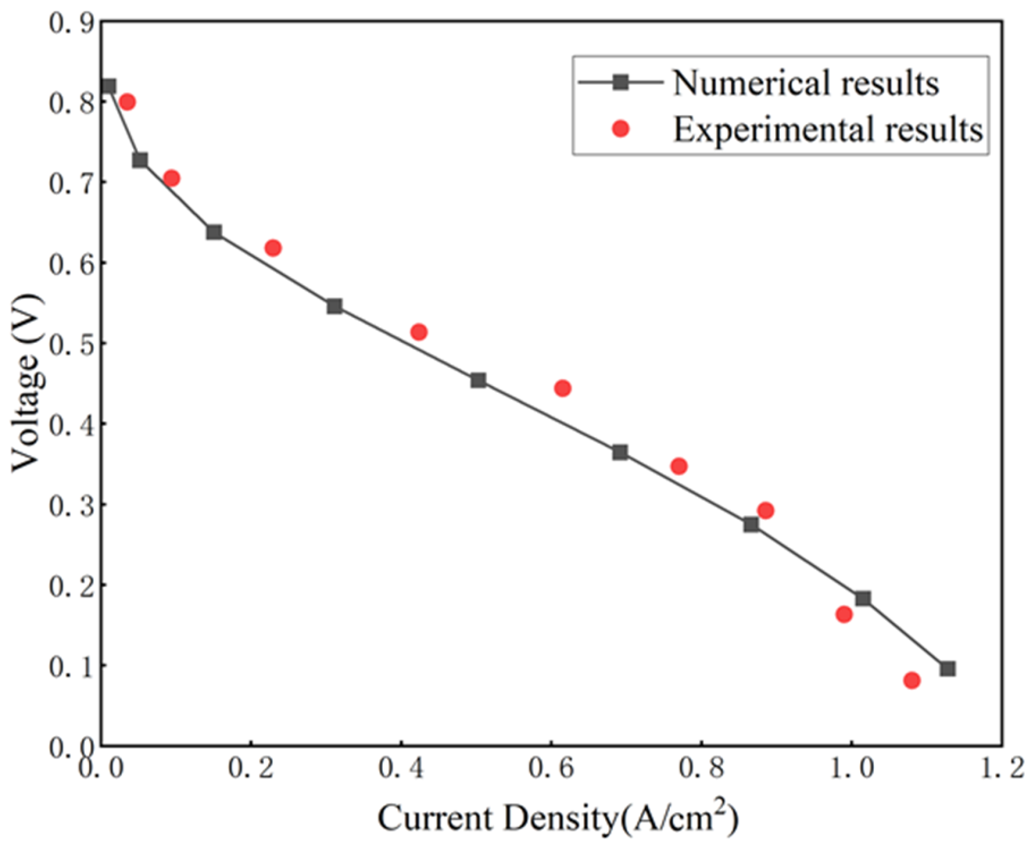
3.1.2. Validation and Grid Independence Test

The grid independence test was performed to reduce the influence of the quantity of grids on the calculation result, as shown in

Table 4. Independence test of grids.

Case	Quantity of Grids	Current Density (A/cm2)
Case1	421,838	4.0918
Case2	610,707	4.0769
Case3	824,345	4.0828
Case4	1,004,194	4.0808
Case5	1,188,828	4.0717

. The density of grids of the model was increased to investigate the influence by comparing the current density of the PEMFC with different quantities of grids. Five cases with five quantities of grids (421,838, 610,707, 824,345, 1,004,194, 1,188,828) were calculated. The largest error of current density between Case1 and Case5 was 0.49%. The quantity of 610,707 grids was applied considering the accuracy and resource of the calculation.

To validate this model, the numerical results were contrasted with the experimental results of Wang [9] because of the similar geometry and operating conditions. The numerical results fit well with the experimental results when the current density was less than 0.9 A/cm², as shown in Figure 3. The numerical results were slightly higher than the experimental results with the increase in current density. The reason was the difference in water formation and distribution between the simulation and reality.

3.1.3. Object of Optimization

L_f and H were chosen to be the decision variables as the key structural parameters of trapezoidal baffles, shown in Figure 1c and Table 2. The reason is that L_f determines the angle between the fluid and the trapezoidal baffles, and H determines the throttle effect of the trapezoidal baffles on the fluid. The values of L_f and H were limited to keep the model running correctly and the rationality of parameters as shown in Equations (19) and (20).

$$0\le L_f\le 4.0,$$

(19)

$$0.2\le H\le 0.4,$$

(20)

The net power density (P_net) is a straightforward criterion to judge the performance of a fuel cell because the net power density reflects the output of the fuel cell and the consumption of the attachment. Therefore, the net power density was chosen to be optimized as the objective function of the trapezoidal baffles. The relationship is shown in Equations (21)–(23).

$$P_{net}=P_{cell}-P_{pump},$$

(21)

$$P_{\mathrm{cell}}=V_{cell}{I}_{ave}{A}_{act},$$

(22)

$$P_{pump}=\Delta P_{ca}{V}_{ca}{A}_{in,ca},$$

(23)

ΔP_ca is the total pressure drop of the cathode flow field. V_ca is the velocity of the fluid in the cathode flow channels. A_{in, ca} is the area of the cathode inlet. A_act is the active area of the cathode. I_ave is the average current density, and V_cell is the working voltage of the PEMFC.

3.1.4. Design of the Database for Training

The database for training the ANN surrogate models was designed by the Latin hypercube sampling (LHS) method, which is an effective stratified random sampling method. The steps of LHS are shown below.

• Determine N, the sample number of the database.
• Divide the interval from 0 to 1 into N equal parts.
• Select a random value in every part of the interval from 0 to 1.
• Map the selected value to the sample of standard normal distribution (SND) by the inverse function of SND.

N in this paper was set to 200 according to the range of variables (L_f and H). The geometric models would be rebuilt and applied to numerical models according to every sample. A database containing all of the variables and calculation results for training the ANN surrogate models was finished.

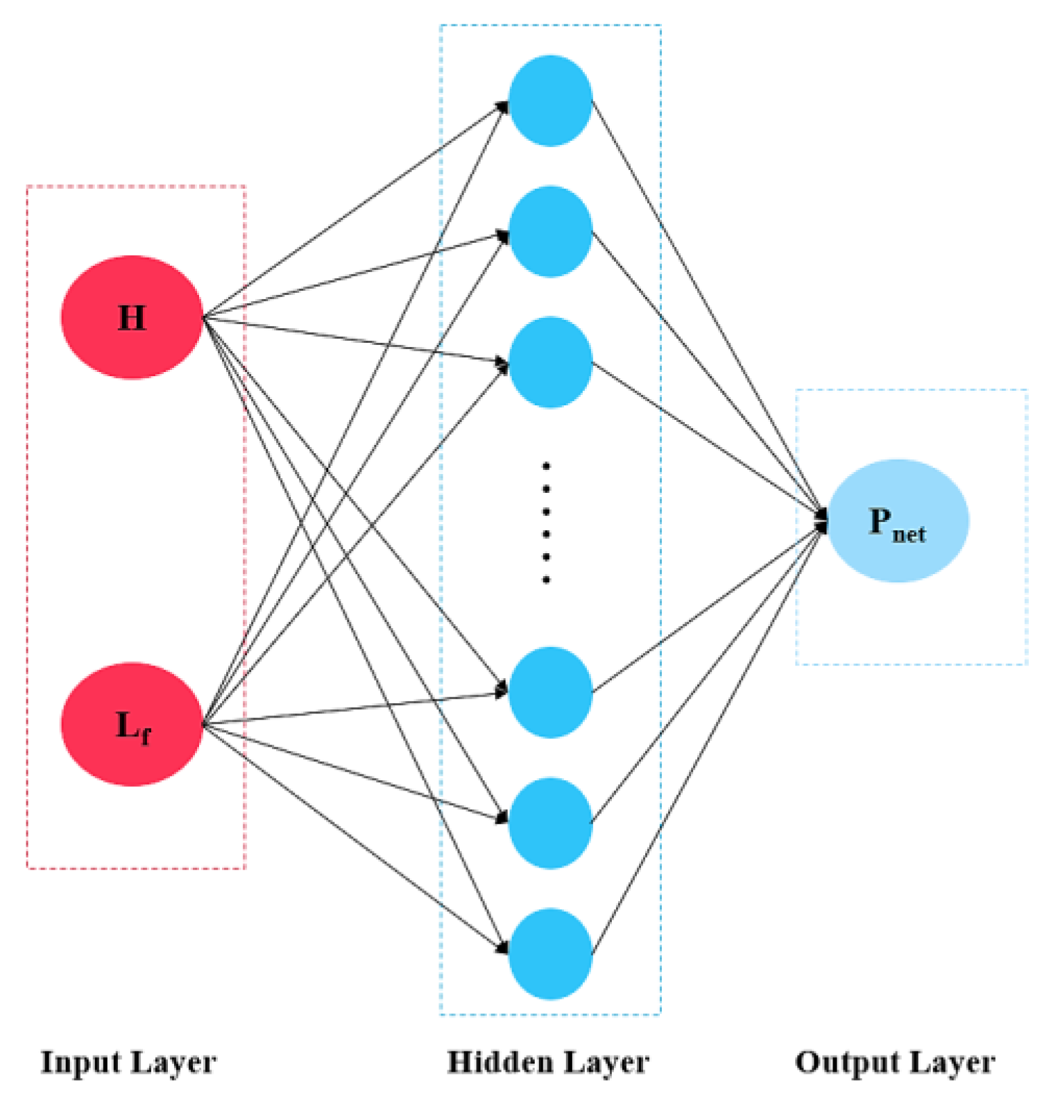
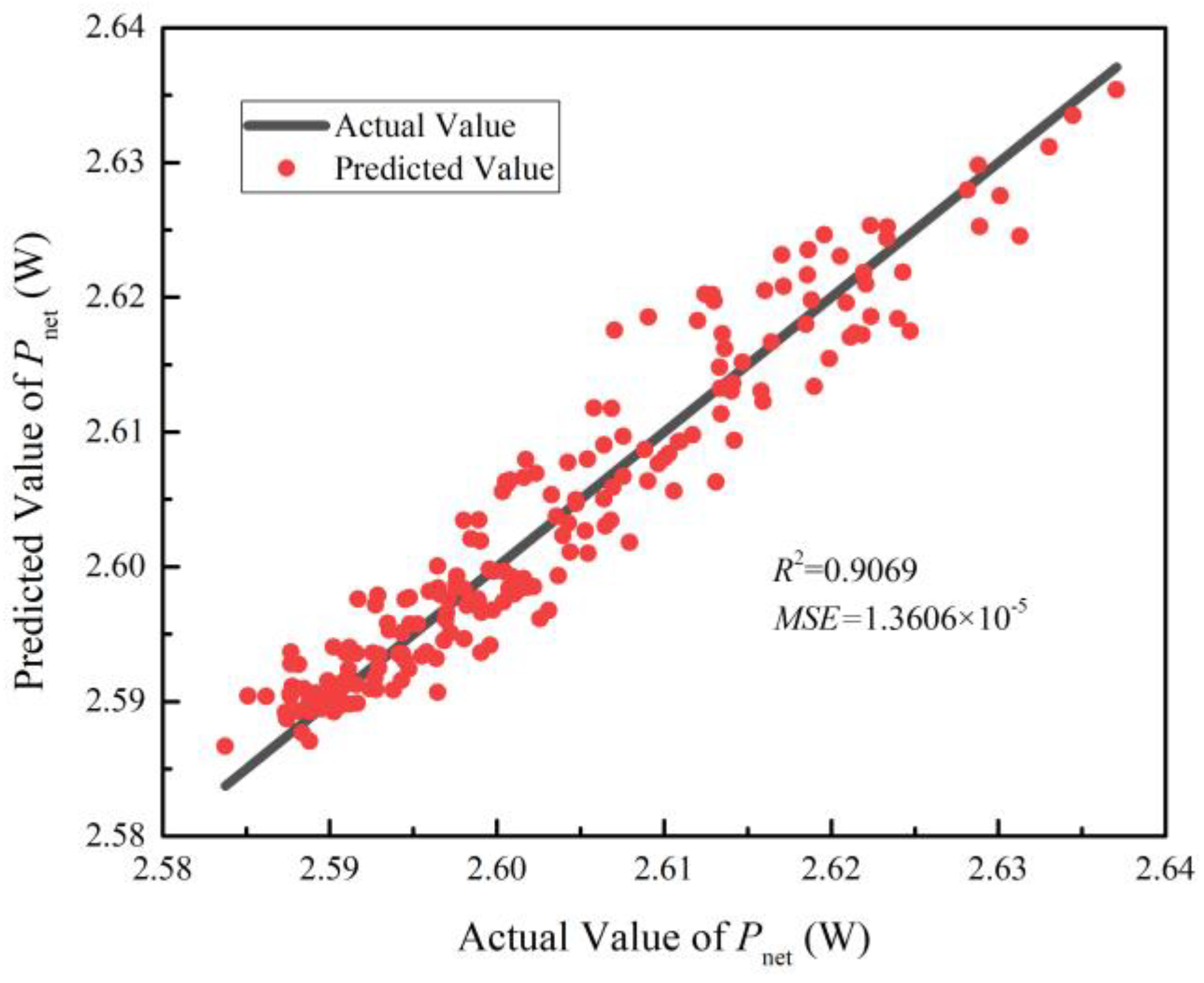
3.1.5. ANN Surrogate Models

The ANN model is a Single-layer Feed-Forward Back Propagation network in this paper. The ANN model consists of an input layer, a hidden layer with 10 neurons, and an output layer. The signal is transferred forward layer by layer. The result of the output layer would be compared with the experimental results, and the error would be transferred back to the hidden layer. The schematic diagram, training parameters, and structural parameters of the ANN models are shown in Figure 4 and

Table 5. Training parameters and structural parameters of the ANN model.

Parameters	Value or Setting
Training set	70%
Test set	15%
Verification set	15%
Neuron number in input layer	2
Neuron number in hidden layer	10
Neuron number in output layer	1
Train function	Levenberg–Marquardt
Activation transfer function	Sigmoid

.

The mean square error (MSE) and coefficient of determination (R²) were applied to evaluate the prediction performance of the ANN model, as shown in Equations (24) and (25).

$$MSE=\frac{1}{n}{\displaystyle \sum _{i=1}^n(f_i}-y_i{)}^2,$$

(24)

$$R^2=1-\frac{{\displaystyle \sum _{i=1}^n{(y_i-f_i)}^2}}{{\displaystyle \sum _{i=1}^n{(y_i-\overline{y_i})}^2}},$$

(25)

n is the N, the sample number, in Section 3.1.4. f_i is the predicted value, $y_i$ is the actual value, and $\overline{y_i}$ is the average value of $y_i$. A small value of MSE and approximate value of R² to 1 indicated precise prediction performance of the ANN model.

The comparison of the predicted value and the actual value showed good prediction performance, as shown in Figure 5. The MSE and R² were 1.3606 × 10⁻⁵ and 0.9069, respectively, which means that the surrogate model trained by ANN was sufficient to predict the P_net in the actual model.

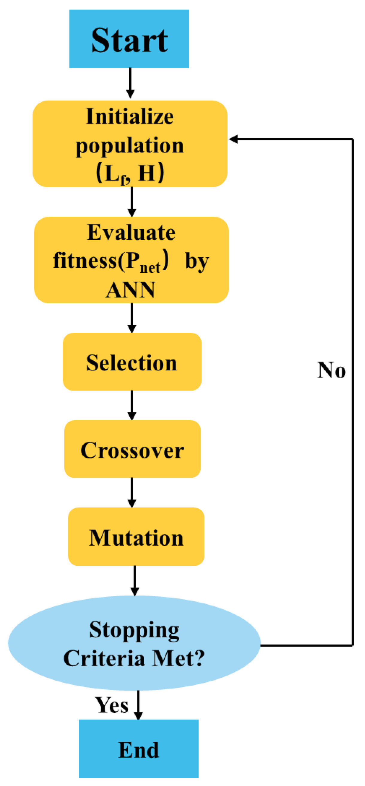
3.1.6. Single-Objective Optimization

The genetic algorithm (GA) was applied to the single-objective optimization as shown in Figure 6. The parameters of GA are shown in

Table 6. The parameters of GA.

Parameters	Values
Population size	50
Evolution generation	180
Crossover fraction	0.8
Mutation fraction	0.01

.

The results of the single-objective optimization are shown in

Table 7. Results of the single-objective optimization.

Results	Values	Unit
Lf	3.0344	mm
H	0.3999	mm
Predicted net power density	2.6357	W/cm2
Calculated net power density	2.6294	W/cm2

. The predicted value of net power density was 2.6357 W/cm² when the values of L_f and H were 3.0344 and 0.3999, respectively. The calculated value for net power density was 2.6294 with the optimized values of L_f and H. The relative error of the predicted value and the calculated value was 0.24%, which indicated good credibility of the surrogate model trained by ANN and optimized by GA.

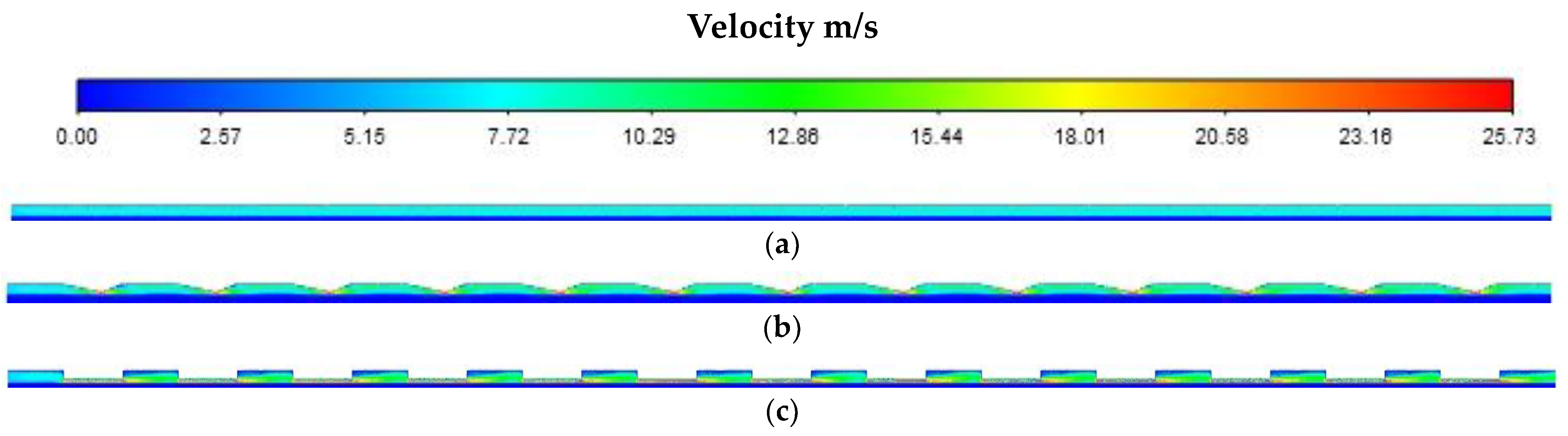
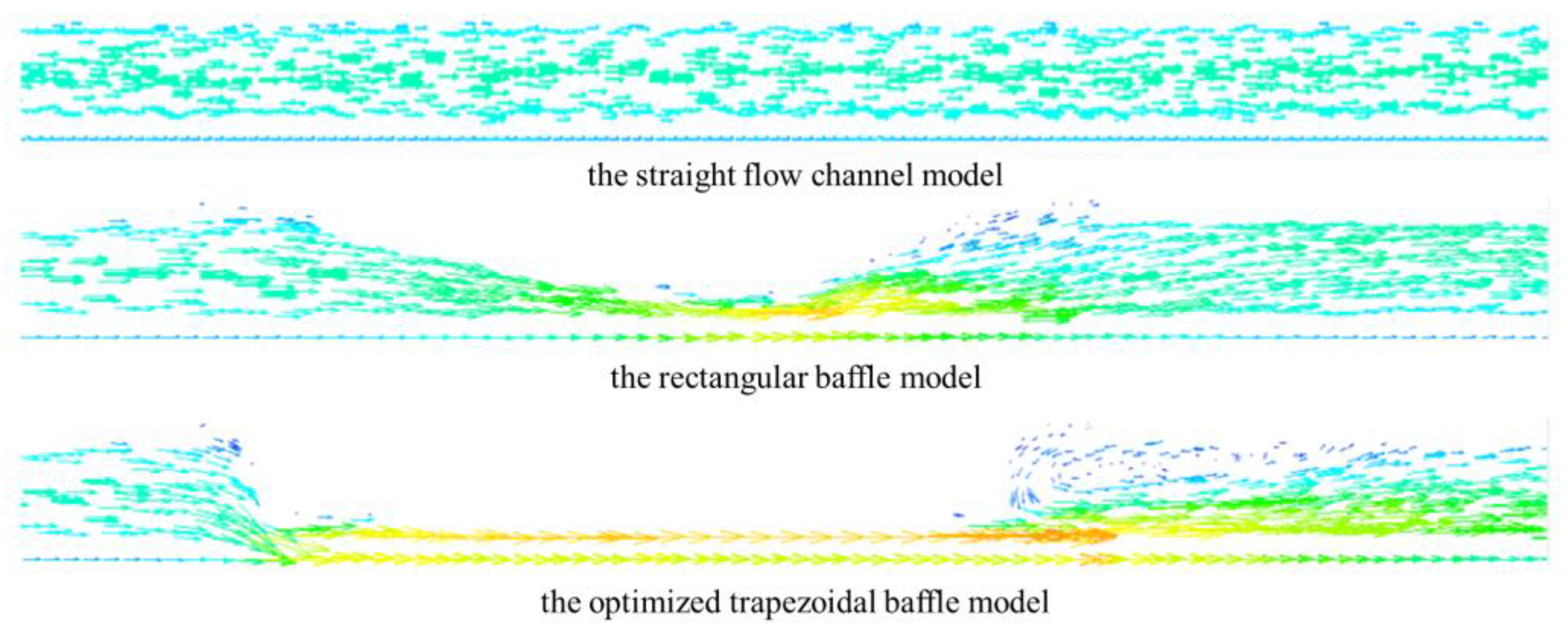
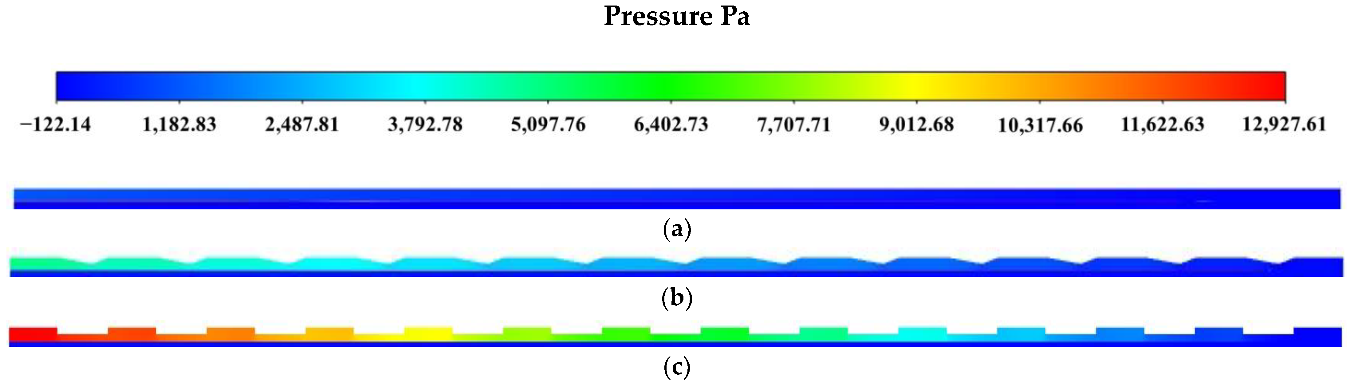
3.2. Comparison and Analysis

In this section, a comparison is presented for the PEMFC models with straight flow channels, optimized trapezoidal baffles, and rectangular baffles (hereinafter, straight flow channel model, optimized trapezoidal baffle model, and rectangular baffle model).

Figure 7 shows the gas velocity distribution contour along the oxygen flow in the three models at 0.4 V. As can be seen from the figure, the gas velocity in the straight flow channel model remained almost constant. The flow velocity of the optimized trapezoidal and rectangular baffle models varied periodically according to their geometry. Figure 8 is a detailed vector diagram of the velocity in the three models at the same distance to the inlet at 0.4 V. In the straight flow channel, most of the velocity vectors point in the axis direction and are thus parallel with the gas diffusion layer. The reaction of the PEMFC is hindered by the inevitable uneven oxygen concentration along the channel. In the optimized trapezoidal baffle model and rectangular baffle model, baffles disturb the uniform oxygen flow, creating turbulence adjacent to the baffles that directs more oxygen towards the gas diffusion layer. Moreover, the throttling effect of the baffles on the airflow increases the flow rate below the baffles, forming a local low-pressure area, which is also conducive to droplet removal on the gas diffusion layer and liquid discharging in the flow channel.

Also shown in Figure 8, there is visible boundary layer separation and vortex generation upstream and downstream of the rectangular baffle—especially downstream, where significant backflow zones are formed, which will significantly increase the required pump power. Figure 9 shows the pressure distribution contour along the oxygen flow in the three models at 0.4 V. In all three models, the pressure decreases gradually along the flow direction. The pressure drop is drastic along the flow direction in the rectangular baffle model, while the pressure drop of the optimized trapezoidal baffle model is moderate.

Figure 10 is the oxygen concentration at the cathode GDL/CL interface in the three models at 0.4 V. The distribution of the oxygen concentration in all three models is generally similar and peaks at the inlet and gradually decreases along the channel. In the rectangular baffle model, the oxygen concentration at the position of the baffles is significantly higher than in the adjacent area, while the adjacent area still has a higher concentration than the straight flow channel model. This improved the oxygen concentration along the whole channel and especially improved the reaction in the latter part of the channel. In the optimized trapezoidal baffle model, the oxygen distribution was similar to that of the rectangular baffle model, with a less significant increase around the baffle, which resulted in better oxygen uniformity.

The oxygen concentration in Figure 10 is statistically given in Figure 11. The straight flow channel had the lowest concentration of the three, while the other two models had periodically increased oxygen concentrations along the flow. The concentration variations in the rectangular baffle model included higher and sharper oxygen concentration increases near the baffles, which improved the chemical reaction at the GDL at the cost of sharper pressure loss, as shown in Figure 9. The optimized trapezoidal baffle model had a relatively gradual oxygen concentration increase, which improved oxygen uniformity along the flow channel.

Figure 12 shows the current flux density at the cathode GDL/CL interface in the three models. In all three models, the current density at the oxygen flow channel outlet was relatively low, since the oxygen concentration was low at the channel outlet due to consumption along the channel. The hydrogen concentration was also low at its flow channel outlet, which in turn resulted in the low current density at the oxygen flow channel inlet. The current flux density near the ribs of bipolar plates was greater than that at the flow channel. This is because electrochemical reactions require a complete circuit, and more negative charges accumulate near the bipolar plates than in the flow channel, making it easier to react with protons that pass through the proton exchange membrane. The central area with sufficient concentrations of both oxygen and hydrogen had a higher current flux density. The current density of the rectangular baffle model was the highest, with significantly higher current density near the baffles, caused by the high oxygen concentration. The current density of the optimized trapezoidal baffle model was lower than that of the rectangular baffle model, while compensating with better uniformity.

Figure 13 shows the H₂O concentration at the cathode GDL/CL interface in the three models. The concentration of water molecules in the straight flow channel model gradually increased along the flow direction, since water generated in the electrochemical reaction gradually accumulated downstream. The other two models had a generally similar distribution; the major difference between the two and the straight flow channel was the higher H₂O concentration downstream of the baffles. The reason for this concentration was the high oxygen concentration and current flux density downstream of the baffles, which resulted in increased water molecule generation. It was also observed that the optimized trapezoidal baffle model had better uniformity in its H₂O concentration compared with the rectangular baffle model.

The H₂O concentration in Figure 13 is statistically given in Figure 14. In the straight flow channel, the H₂O concentration in the first half was visibly higher than in the other two models, while visibly lower in the second half. In the straight flow channel model, the water discharging process was limited by the smooth oxygen flow, while in the other two models, the baffle structure improved the process, so the molar concentration of water in the first half of the straight flow channel was slightly higher than that of the other two models. This caused the difference in the first half. In the two models with baffles, on one hand, due to the existence of the baffles, the oxygen concentration in the flow channel was higher on average, which resulted in a larger amount of water generation; on the other hand, the baffle structure improved the water discharging process within the flow channel, which in turn discharged water from upstream to downstream. Therefore, in the second half of the flow channel, the molar concentration of water in the other two models was slightly higher.

4. Discussion

Figure 15 and Figure 16 show comparisons of the polarization curves and power density curves of the straight flow channel model, the rectangular baffle model, and the trapezoidal baffle model. As can be seen from the figures, the performance difference between the three models was insignificant at higher voltage. However, at lower voltage with higher current density, the performance of the rectangular baffle model visibly surpassed that of the other two. The power density was 8.3% higher than in the straight flow channel model at a voltage of 0.3 V. In the optimized trapezoidal baffle model, it was 4.0% higher than that in the straight flow channel model.

The rectangular baffle model had obvious advantages in term of the polarization curve and power density. However, it also caused more pressure loss, as shown in Figure 17. When the current density was 4 A/cm², the pressure drop of the straight flow channel model was 1377 Pa, while the pressure drop of the rectangular baffle model was about 12,938 Pa, which was 938.9% that of the straight flow channel model. Although the pressure drop of the optimized trapezoidal baffle model was also greater than that of the straight flow channel model, the pressure drop of 4895 Pa was only 37.83% that of the rectangular baffle model.

Higher pressure losses accordingly require higher pumping power. In practice, the limited pump efficiency will further increase the practical pump power requirement. The net power output of the PEMFC after considering the pump power consumption is shown in Figure 18. The comparison is based on voltages of 0.4 V and 0.6 V; the former yielded the highest power density, and the latter was closer to the practical requirement of an on-road PEMFC. At 0.4 V, due to the large power density of the PEMFC and the limited change in pump power, the influence of pump efficiency was relatively low. With pump efficiency higher than 30%, the net power output of the rectangular baffle model was better than that of the optimized trapezoidal baffle model. However, at 0.6 V, the advantage of the trapezoidal baffle significantly increased; the model had a net power increase of 1.47% compared to the rectangular baffle model at 50% pump efficiency and 3.94% at 30% pump efficiency. Considering the pump efficiency in reality, the optimized trapezoidal baffle model could improve the performance of the fuel cell better than the rectangular baffle model and showed an oxygen distribution similar to that of the rectangular baffle model.

5. Conclusions

In this paper, a flow channel with a trapezoidal baffle was suggested, and geometric parameters of the baffle were optimized based on CFD simulation, ANN, and single-objective optimization methods, to improve the net power output of the PEMFC.

• A flow channel model with trapezoidal baffle was suggested, and a 3D and multi-phase CFD model of the PEMFC was established. The ANN method was used to train the surrogate model, and the single-objective optimization method was used to optimize the geometric parameters of the trapezoidal baffle, and the CFD model and the ANN model were verified, respectively.
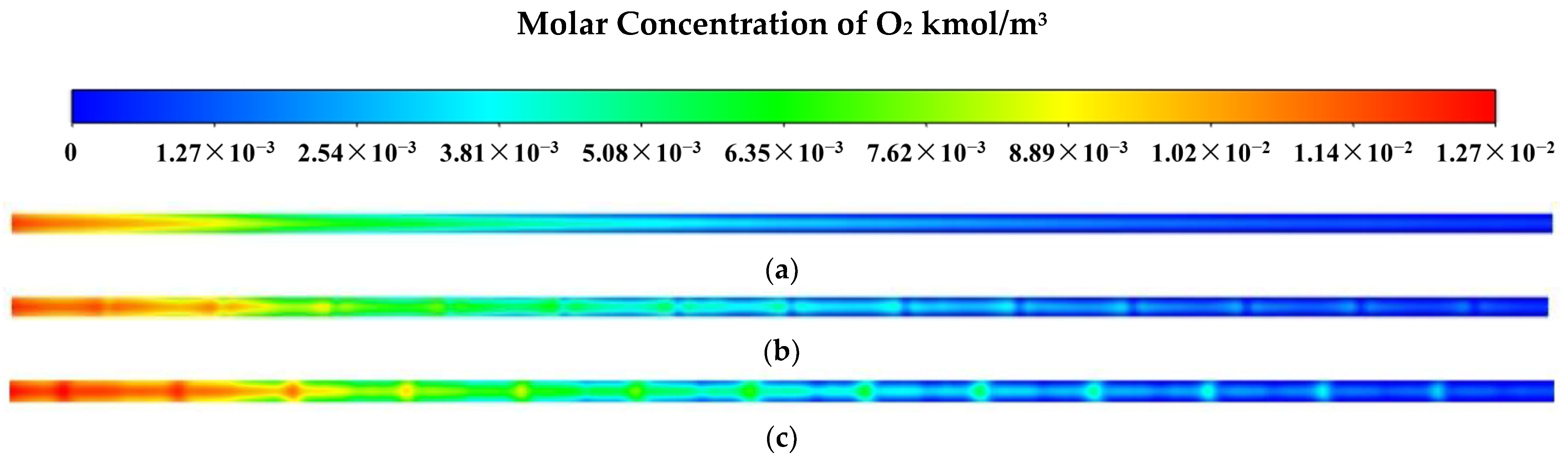
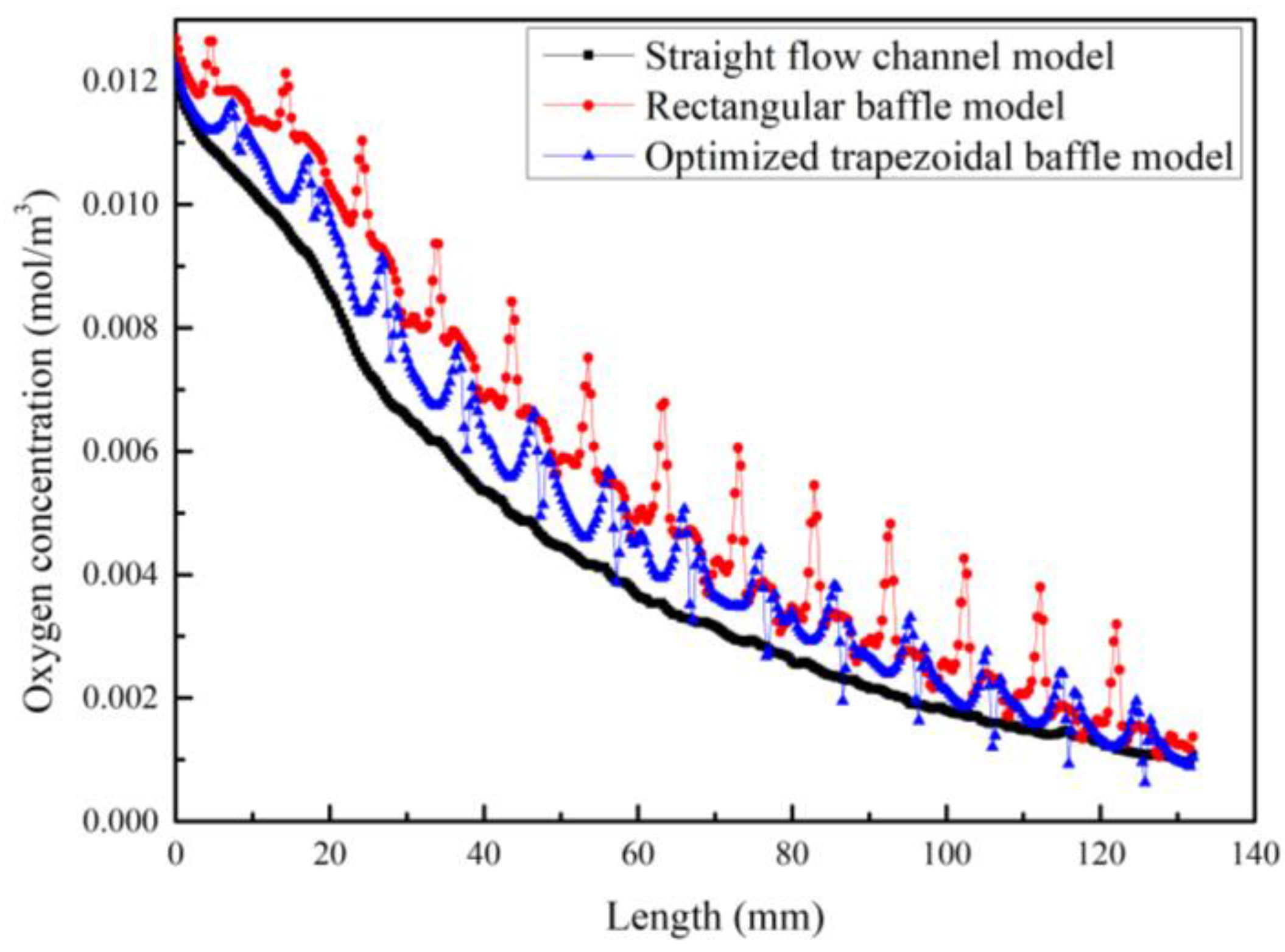
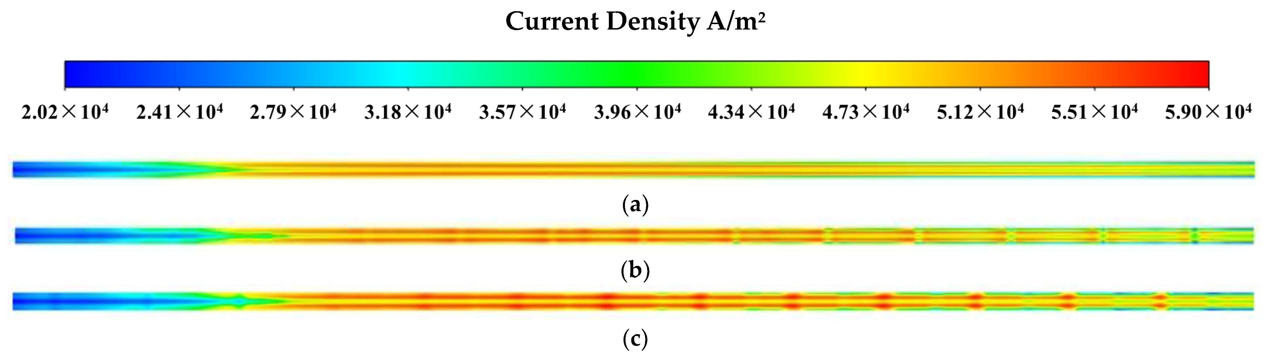
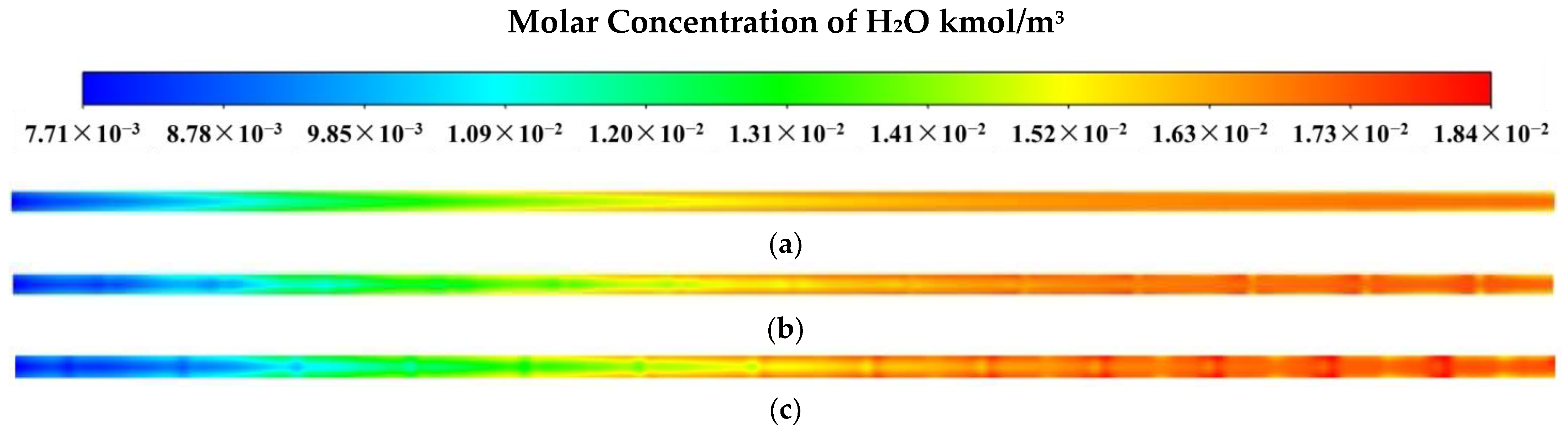
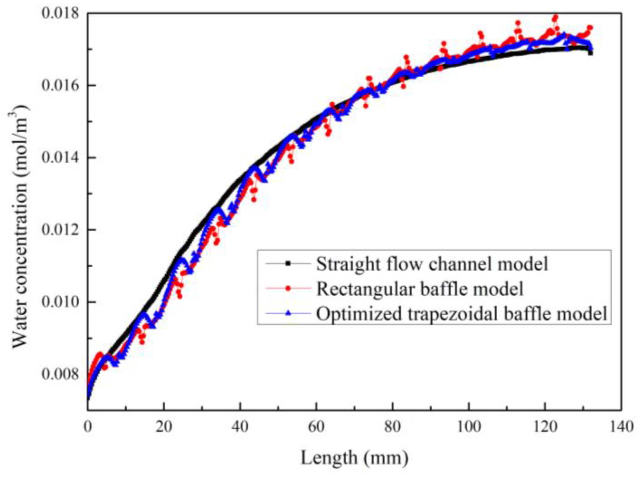
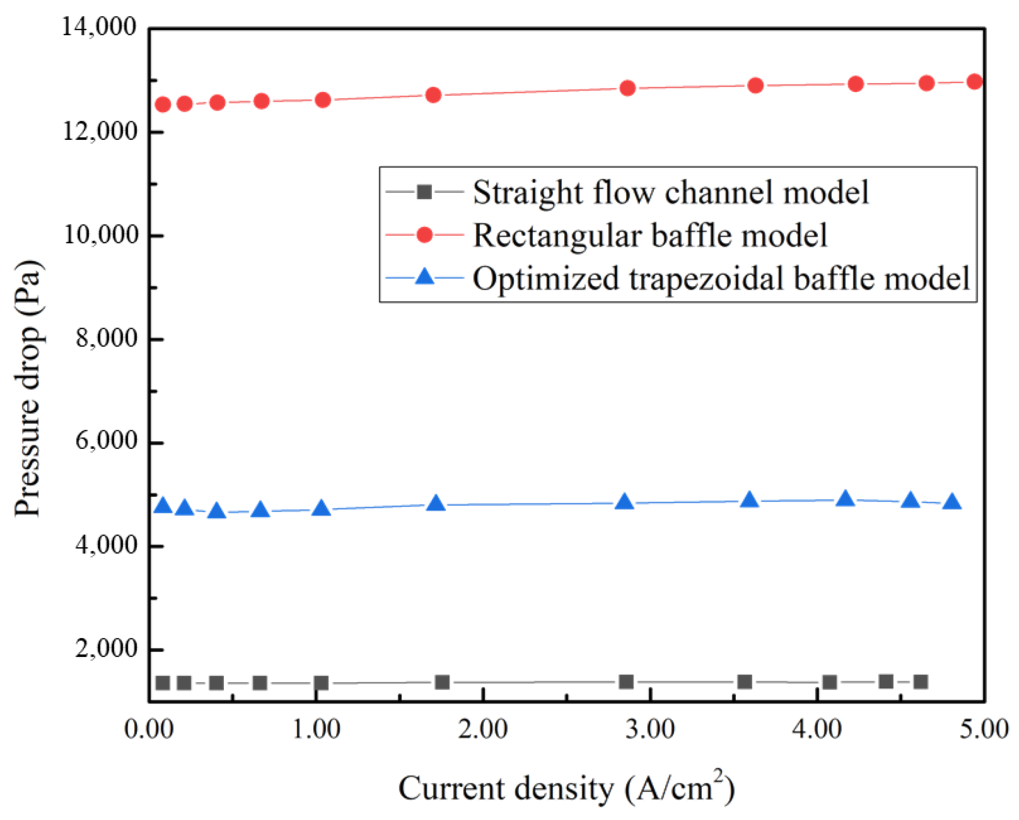
• The velocity, pressure, and oxygen distribution in the straight flow channel model, rectangular baffle model, and the optimized trapezoidal baffle model were analyzed, and the results showed that the optimized trapezoidal baffle model can effectively improve the transport of oxygen towards the GDL. With voltage at 0.3 V, the power density of the optimized model was 4.0% higher than that of the straight flow channel model, and the pressure drop was only 37.83% that of the rectangular baffle model. The optimized trapezoidal baffle model showed better performance than the straight flow channel model and less pressure drop than the rectangular baffle model.
• The PEMFC had its highest power output with a voltage of 0.4 V. The rectangular baffle model with higher power density can achieve higher net power output than the trapezoidal baffle model, even with relatively high pump power requirements. However, for on-road PEMFC with 0.6 V voltage, the influence of pump power was significant, and the optimized trapezoidal baffle model had a net power increase of 1.47% compared to the rectangular baffle model at 50% pump efficiency and 3.94% at 30% pump efficiency. The performance of the optimized trapezoidal baffle model surpassed that of the other two models in practical application.

References

1. Barbir, F.; Yazici, S. Status and development of PEM fuel cell technology. Int. J. Energy Res. 2008, 32, 369–378. [Google Scholar] [CrossRef]
2. Manoharan, Y.; Hosseini, S.E.; Butler, B.; Alzhahrani, H.; Senior, B.T.F.; Ashuri, T.; Krohn, J. Hydrogen Fuel Cell Vehicles; Current Status and Future Prospect. Appl. Sci. 2019, 9, 2296. [Google Scholar] [CrossRef]
3. Wang, Y.; Diaz, D.F.R.; Chen, K.S.; Wang, Z.; Adroher, X.C. Materials, technological status, and fundamentals of PEM fuel cells—A review. Mater. Today 2020, 32, 178–203. [Google Scholar] [CrossRef]
4. Ijaodola, O.S.; El-Hassan, Z.; Ogungbemi, E.; Khatib, F.N.; Wilberforce, T.; Thompson, J.; Olabi, A.G. Energy efficiency improvements by investigating the water flooding management on proton exchange membrane fuel cell (PEMFC). Energy 2019, 179, 246–267. [Google Scholar] [CrossRef]
5. Jiao, K.; Li, X. Water transport in polymer electrolyte membrane fuel cells. Prog. Energy Combust. Sci. 2011, 37, 221–291. [Google Scholar] [CrossRef]
6. Wang, X.R.; Ma, Y.; Gao, J.; Li, T.; Jiang, G.Z.; Sun, Z.Y. Review on water management methods for proton exchange membrane fuel cells. Int. J. Hydrogen Energy 2020, 46, 12206–12229. [Google Scholar] [CrossRef]
7. Lin, R.; Ren, Y.S.; Lin, X.W.; Jiang, Z.H.; Yang, Z.; Chang, Y.T. Investigation of the internal behavior in segmented PEMFCs of different flow fields during cold start process. Energy 2017, 123, 367–377. [Google Scholar] [CrossRef]
8. Pei, H. Study on Water And Heat Management of PEMFC. Ph.D. Thesis, Huazhong University, Wuhan, China, 2014. [Google Scholar]
9. Wang, L.; Husar, A.; Zhou, T.; Liu, H. A parametric study of PEM fuel cell performances. Int. J. Hydrogen Energy 2003, 28, 1263–1272. [Google Scholar] [CrossRef]
10. Hakenjos, A.; Muenter, H.; Wittstadt, U.; Hebling, C. A PEM fuel cell for combined measurement of current and temperature distribution, and flow field flooding. J. Power Sources 2004, 131, 213–216. [Google Scholar] [CrossRef]
11. Nandjou, F.; Poirot-Crouvezier, J.-P.; Chandesris, M.; Blachot, J.-F.; Bonnaud, C.; Bultel, Y. Impact of heat and water management on proton exchange membrane fuel cells degradation in automotive application. J. Power Sources 2016, 326, 182–192. [Google Scholar] [CrossRef]
12. Sakaida, S.; Tabe, Y.; Chikahisa, T. Large scale simulation of liquid water transport in a gas diffusion layer of polymer electrolyte membrane fuel cells using the lattice Boltzmann method. J. Power Sources 2017, 361, 133–143. [Google Scholar] [CrossRef]
13. Shao, Y.; Xu, L.; Li, J.; Hu, Z.; Fang, C.; Hu, J.; Guo, D.; Ouyang, M. Hysteresis of output voltage and liquid water transport in gas diffusion layer of polymer electrolyte fuel cells. Energy Convers. Manag. 2019, 185, 169–182. [Google Scholar] [CrossRef]
14. Shao, Y.; Xu, L.; Li, J.; Ouyang, M. Numerical modeling and performance prediction of water transport for PEM fuel cell. Energy Procedia 2019, 158, 2256–2265. [Google Scholar] [CrossRef]
15. Zhao, J.; Li, X. Oxygen transport in polymer electrolyte membrane fuel cells based on measured electrode pore structure and mass transport properties. Energy Convers. Manag. 2019, 186, 570–585. [Google Scholar] [CrossRef]
16. Peng, Y.; Mahyari, H.M.; Moshfegh, A.; Javadzadegan, A.; Toghraie, D.; Shams, M.; Rostami, S. A transient heat and mass transfer CFD simulation for proton exchange membrane fuel cells (PEMFC) with a dead-ended anode channel. Int. Commun. Heat Mass Transf. 2020, 115, 104638. [Google Scholar] [CrossRef]
17. Peng, Y.; Yan, X.; Lin, C.; Shen, S.; Yin, J.; Zhang, J. Effects of flow field on thermal management in proton exchange membrane fuel cell stacks: A numerical study. Int. J. Energy Res. 2021, 45, 7617–7630. [Google Scholar] [CrossRef]
18. Li, T.; Song, J.H.; Ke, Z.; Lin, G.; Qu, G.; Song, Y. Research on new flow channel design for improving water management ability of proton exchange membrane fuel cell. J. Mater. Sci. 2022, 57, 6669–6687. [Google Scholar] [CrossRef]
19. Luo, X.; Chen, S.; Xia, Z.; Zhang, X.; Yuan, W.; Wu, Y. Numerical Simulation of a New Flow Field Design with Rib Grooves for a Proton Exchange Membrane Fuel Cell with a Serpentine Flow Field. Appl. Sci. 2019, 9, 4863. [Google Scholar] [CrossRef]
20. Saripella, B.P.; Koylu, U.O.; Leu, M.C. Experimental and Computational Evaluation of Performance and Water Management Characteristics of a Bio-Inspired Proton Exchange Membrane Fuel Cell. J. Fuel Cell Sci. Technol. 2015, 12, 061007. [Google Scholar] [CrossRef]
21. Zamora-Antunano, M.A.; Pimentel, P.E.O.; Orozco-Gamboa, G.; Garcia-Garcia, R.; Olivarez-Ramirez, J.M.; Santos, E.R.; Baltazar, A.D.R. Flow Analysis Based on Cathodic Current Using Different Designs of Channel Distribution in PEM Fuel Cells. Appl. Sci. 2019, 9, 3615. [Google Scholar] [CrossRef]
22. Ghasabehi, M.; Ashrafi, M.; Shams, M. Performance analysis of an innovative parallel flow field design of proton exchange membrane fuel cells using multiphysics simulation. Fuel 2020, 285, 119194. [Google Scholar] [CrossRef]
23. Zhou, Y.; Chen, B.; Chen, W.; Deng, Q.; Shen, J.; Tu, Z. A novel opposite sinusoidal wave flow channel for performance enhancement of proton exchange membrane fuel cell. Energy 2022, 261, 125383. [Google Scholar] [CrossRef]
24. Ebrahimzadeh, A.; Khazaee, I.; Fasihfar, A. Experimental and numerical investigation of obstacle effect on the performance of PEM fuel cell. Int. J. Heat Mass Transf. 2019, 141, 891–904. [Google Scholar] [CrossRef]
25. Dong, P.; Xie, G.; Ni, M. The mass transfer characteristics and energy improvement with various partially blocked flow channels in a PEM fuel cell. Energy 2020, 206, 117977. [Google Scholar] [CrossRef]
26. Li, Z.J.; Wang, S.B.; Li, W.W.; Zhu, T.; Xie, X.F. Wavy channels to enhance the performance of proton exchange membrane fuel cells. J. Tsinghua Univ. Sci. Technol. 2021, 10, 1046–1054. [Google Scholar] [CrossRef]
27. Girimurugan, R.; Anandhu, K.; Thirumoorthy, A.; Harikrishna, N.; Makeshwaran, E.; Prasanna, S.; Krishnaraj, R. Performance studies on proton exchange membrane fuel cell with slightly tapered single flow channel for dissimilar cell potentials. Mater. Today Proc. 2023, 74, 602–610. [Google Scholar] [CrossRef]
28. Zhang, G.; Guan, Z.; Li, D.; Li, G.; Bai, S.; Sun, K.; Cheng, H. Optimization Design of a Parallel Flow Field for PEMFC with Bosses in Flow Channels. Energies 2023, 16, 5492. [Google Scholar] [CrossRef]
29. Ming, W.; Sun, P.; Zhang, Z.; Qiu, W.; Du, J.; Li, X.; Zhang, Y.; Zhang, G.; Liu, K.; Wang, Y.; et al. A systematic review of machine learning methods applied to fuel cells in performance evaluation, durability prediction, and application monitoring. Int. J. Hydrogen Energy 2023, 48, 5197–5228. [Google Scholar] [CrossRef]
30. Cao, J.; Yin, C.; Feng, Y.; Su, Y.; Lu, P.; Tang, H. A Dimension-Reduced Artificial Neural Network Model for the Cell Voltage Consistency Prediction of a Proton Exchange Membrane Fuel Cell Stack. Appl. Sci. 2022, 12, 11602. [Google Scholar] [CrossRef]
31. Qiu, Y.; Wu, P.; Miao, T.; Liang, J.; Jiao, K.; Li, T.; Lin, J.; Zhang, J. An Intelligent Approach for Contact Pressure Optimization of PEM Fuel Cell Gas Diffusion Layers. Appl. Sci. 2020, 10, 4194. [Google Scholar] [CrossRef]
32. Yu, Z.; Xia, L.; Xu, G.; Wang, C.; Wang, D. Improvement of the three-dimensional fine-mesh flow field of proton exchange membrane fuel cell (PEMFC) using CFD modeling, artificial neural network and genetic algorithm. Int. J. Hydrogen Energy 2022, 47, 35038–35054. [Google Scholar] [CrossRef]
33. Ansys Fluent: A History of Innovations in CFD. Available online: https://www.ansys.com/zh-cn/blog/ansys-fluent-history-of-innovations (accessed on 29 September 2022).
34. Tian, W.; VanGilder, J.; Condor, M.; Ardolino, A. Comparison of Time-Splitting and SIMPLE Pressure-Velocity Coupling for Steady-State Data Center CFD. In Proceedings of the IEEE Intersociety Conference on Thermal and Thermomechanical Phenomena in Electronic Systems (ITherm), Orlando, FL, USA, 30 May–2 June 2023. [Google Scholar]
Figure 1. Schematic diagrams of the CFD model: (a) Structure of the single fuel cell. (b) Computational domain of the cathode flow channel with baffles. (c) Configuration of trapezoidal baffles.
Applsci 14 00428 g001
Figure 2. The grid of the model and the partial magnification (50×).
Applsci 14 00428 g002
Figure 3. Contrast between the numerical and experimental results.
Applsci 14 00428 g003
Figure 4. Schematic diagram of the ANN model.
Applsci 14 00428 g004
Figure 5. Comparison of the predicted value and the actual value.
Applsci 14 00428 g005
Figure 6. Schematic diagram of single-objective optimization.
Applsci 14 00428 g006
Figure 7. Velocity distribution of air inflow channels. (a) The straight flow channel model; (b) the rectangular baffle model; (c) the optimized trapezoidal baffle model.
Applsci 14 00428 g007
Figure 8. Vector diagram of velocity of air inflow channels.
Applsci 14 00428 g008
Figure 9. Pressure distribution of air inflow channels. (a) The straight flow channel model; (b) the rectangular baffle model; (c) the optimized trapezoidal baffle model.
Applsci 14 00428 g009
Figure 10. Oxygen concentration at the cathode GDL/CL interface. (a) The straight flow channel model; (b) the rectangular baffle model; (c) the optimized trapezoidal baffle model.
Applsci 14 00428 g010
Figure 11. Oxygen concentration at the cathode GDL/CL interface around the axis of symmetry.
Applsci 14 00428 g011
Figure 12. Current flux density at the cathode GDL/CL interface. (a) The straight flow channel model; (b) the rectangular baffle model; (c) the optimized trapezoidal baffle model.
Applsci 14 00428 g012
Figure 13. H2O concentration at the cathode GDL/CL interface. (a) The straight flow channel model; (b) the rectangular baffle model; (c) the optimized trapezoidal baffle model.
Applsci 14 00428 g013
Figure 14. Water concentration at the cathode GDL/CL interface around the axis of symmetry.
Applsci 14 00428 g014
Figure 15. Polarization curves for three models.
Applsci 14 00428 g015
Figure 16. Power density curves for the three models.
Applsci 14 00428 g016
Figure 17. Pressure drop of flow channels in three models.
Applsci 14 00428 g017
Figure 18. Net power density with different pump efficiencies: (a) at 0.4 V; (b) at 0.6 V.
Applsci 14 00428 g018