Abstract
The use of photovoltaic (PV) panels in interior spaces is expected to increase due to the proliferation of low-power sensor devices in the IoT domain. PV models are critical for estimating the I–V curves that define their performance at various light intensities. These models and the extraction of their parameters have been extensively studied under outdoor conditions, but their indoor illumination performance is less studied. With respect to the latter, several studies have used the parameter-scaling technique. However, the model’s accuracy degrades when the light level decreases. In this study, we propose a simple PV modeling technique that can be applied at various illuminance levels by only using characteristic points (short-circuit current, open-circuit voltage, and maximum-power voltage points) at a reference illumination level. The model uses the characteristic point translation technique to translate the reference characteristic points to other operating conditions. Then, parameter extraction technique is used to extract the model’s parameters. The proposed model’s accuracy is verified using two commercial PV panels and different indoor lighting technologies. The results indicate that the proposed model outperforms the other examined works in terms of accuracy, with an average improvement of 15.75%.
1. Introduction
Renewable energy sources have become an urgent priority as a result of climate change and the fact that a major portion of the energy consumed globally is still generated from fossil fuels [1]. Solar and ambient light are the most promising renewable energy sources, and photovoltaic (PV) panels allow for the most direct conversion of light energy to electrical energy. As a result, photovoltaic technology has attracted extensive interest over the last few decades. PV panels have a wide range of applications, ranging from high-power industrial energy generation to low-power emerging energy harvesting to power Internet of Things (IoT) devices. PV panels are also expected to enable the most economical renewable energy in the near future due to their low and decreasing manufacturing costs [2].
A PV panel is made up of silicon wafer cells that can be connected in series or in parallel to generate the desired voltage and current [3]. The performance of PV panels can be easily determined using the I–V curve. This curve represents the relationship between the output current and the voltage of the PV panel. The equivalent circuit-based models are most commonly used to describe the curve [4]. However, the curve is nonlinear and highly dependent on both irradiance/illuminance levels and temperature. As a result, the complexity of developing an accurate model is high. Nonetheless, an accurate PV model is critical for evaluating the electrical response of different PV panels under a variety of operating conditions that can be encountered in practice.
PV models employ an equivalent circuit with a few parameters that adequately reflect its behavior, and they can be calculated either through optimization or analytical methods. Optimization methods were employed to extract the parameters in [5,6,7,8,9]. However, the accuracy of the extracted parameters is highly dependent on the algorithm type, objective, and initial settings. With an increase in the number of factors, the optimizer’s ability to produce accurate results decreases. Additionally, optimization methods require I–V curve information to determine an optimal match. This may restrict the model’s applicability, as not all panel manufacturers provide information on the I–V curve. A few analytical works have involved the extraction of the model’s parameters solely from datasheet values. Since almost all manufacturers provide datasheet values, the analytical method can be applied to nearly all PV panels. However, the models only work well at the standard irradiance of 1000 W/m2. Therefore, considering that environmental conditions such as irradiance levels might affect the model’s parameters, the studies reported in [10,11,12,13] were conducted using the parameter-scaling technique. The results show significant performance variations with several commercial PV panels at varying irradiance/illuminance levels. Hence, the findings suggest that parameter scaling should not be seen as the primary technique for modeling PV behavior. In [14,15,16,17,18], the characteristic point translation technique was used. This technique can translate three characteristic points from the data sheet to other irradiance levels: short-circuit current, open-circuit voltage, and maximum-power points. However, the accuracy of this characteristic point translation technique can still be improved at low irradiance levels. Moreover, the limited amount of research conducted using the characteristic point translation technique in indoor environments highlights a knowledge deficit with respect to the performance of typical PV models. This deficit constrains our capability to estimate the operation of PV panels and their output power under indoor artificial light. An overview of PV modeling methods is shown in Figure 1.
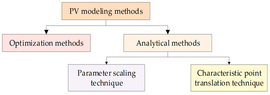
Figure 1.
Overview of PV modeling methods.
The main objective of this work is to develop a PV model with the characteristics of high accuracy in indoor conditions and wide applicability, only requiring characteristic points at a reference illumination. In view of this, a one-diode model with two resistors is chosen to model PV behavior in indoor environments because such a model incorporates a parallel resistor, which is used to represent the leakage current [19]. Compared to other models reported in [20,21,22,23,24,25], the one-diode model provides high accuracy while remaining simple. Furthermore, the proposed model takes a novel approach by applying the characteristic points translation technique to determine the three characteristic points at various illuminance levels. The obtained values are then integrated with the parameter extraction technique to extract the model’s parameters. This approach is expected to improve the proposed model’s accuracy at low light levels. Moreover, it only requires an indoor reference of the three characteristic points as input, and it can model the PV behavior under different operating conditions. To determine the reference value for the model’s input, an experiment is carried out. Various light source technologies are used to illuminate multiple commercial PV panels, and the light intensity is extensively verified using light measurement devices. Several similar works utilizing different techniques are used for comparison purposed to evaluate the expected improvement in accuracy of the proposed model.
2. Methodology
This section is divided into four subsections; the first subsection reviews the one-diode model with two resistors, whereas the second subsection presents the parameter extraction technique. Furthermore, the third subsection describes the characteristic point translation technique, and the fourth subsection presents the experimental and validation procedures.
2.1. One-Diode Model with Two Resistors
The one-diode model was initially developed for one solar cell, but it can be easily extended to include PV panels with multiple cells by incorporating the number of cells in the model. The same model can also be used for both monocrystalline and polycrystalline solar cells [26,27]. Figure 2 illustrates the equivalent circuit for the one-diode model with two resistors. The circuit is composed of the photocurrent source (Iph), the diode, the parallel resistor (Rp), and the series resistor (Rs). Using Kirchhoff’s current law, the output current (I) can be stated as follows with reference to Figure 2:
where Id is the current through the diode and V is the voltage. The diode current can be further represented using the Shockley diode equation, which is as follows:
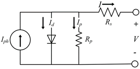
Figure 2.
One-diode model with two resistors.
Hence, the model’s output current equation is described as follows by substituting Equation (2) into Equation (1):
where Io is the diode’s saturation current, q is the charge of an electron, Ns is the number of PV cells that are connected in series, a is the diode’s ideality factor, T is the temperature, and k is the Boltzmann constant.
However, the addition of more variables to the one-diode equation presented in Equation (3) makes the analytical solution impractical. This means that variables I and V in each member cannot be separated and isolated using simple functions [28]. The equation is also known as a transcendental equation, since it is an expression of the form I = f(I,V). Therefore, the Newton–Raphson numerical method is chosen. It is a relatively quick convergence algorithm for computing the roots of a function [29,30,31] and is expressed as:
where xn+1 is the present iteration’s estimated value, xn is the output of the previous iteration, f(x) is the initialized function with xn, and f′(x) is the initialized derivative of xn.
2.2. Parameter Extraction Technique
The model is composed of five parameters: Iph, Io, a, Rs, and Rp. These parameters can be retrieved using the parameter extraction technique described in [12]. To begin, the output current of the model is evaluated using Equation (3) under various operating conditions, including open-circuit, short-circuit, and maximum-power conditions.
Under the open-circuit condition, V = Voc and I = 0. Hence, the output current can be written as:
Under the short-circuit condition, V = 0 and I = Isc. The output current is:
Under the maximum-power condition, V = Vm and I = Im. The output current is:
where Voc represents the open-circuit voltage, Isc represents the short-circuit current, Vm represents the maximum-power voltage, and Im represents the maximum-power current. By rearranging and simplifying the above equations, Iph and Io can be written as:
The authors of [12] included the number of parallel-connected PV cells (Np) in Equation (3) to obtain a more precise expression for the parameters Rs and Rp. The inclusion of Np effectively scales down V to represent the voltage of a single solar cell. The accuracy improvement comes from the knowledge that the voltage of a single solar cell is within a limited range. As a result, the new equation for the model’s output current is as follows:
To obtain the parameter Rs, Equation (10) is assessed under short-circuit, open-circuit, and maximum-power conditions. The expression (VNp + IRsNs)/(NpNsRp) can be omitted due to the low level of current flowing through the parallel resistor, yielding the following:
Furthermore, the formula for Rp can be obtained from the derivative of the current in relation to the voltage at the maximum-power point:
Similarly, the short-circuit and open-circuit conditions in Equation (10) are substituted into Equation (12) to derive the parameter Rp, as shown in Equation (13). The authors of [12] recommended increasing the value of parameter a from 0 until Rp achieves its minimal positive value. After determining the values of the five parameters, the Rs value can be increased iteratively to match the maximum power point, as proposed in [12]. This adjustment of Rs is performed to increase the model’s accuracy. It is noted that the Rs value affects the fill factor and maximum-power point. The higher the Rs value, the lower the fill factor and maximum-power point. Based on the observation that the I–V curve of the PV panel under low indoor illuminance levels has a lower fill factor and maximum-power point compared to under outdoor conditions, the higher Rs value that matches the maximum-power point is able to produce a more accurate I–V curve. By applying this technique, the model’s accuracy can be improved.
The procedure of parameter extraction methods is shown in Figure 3. To begin with, the characteristic point values at the reference illuminance of 1000 lux are obtained and translated. These translated values are used to extract the parameters of the model. Next, the Newton–Raphson method is used to generate the I–V curve. The values of the model are obtained and compared to check its accuracy. The process ends if sufficient accuracy is achieved; otherwise the value of Rs is increased to meet the accuracy requirement.
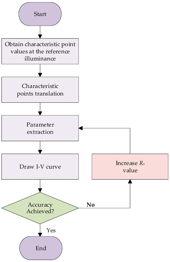
Figure 3.
Flow chart of parameter extraction methods.
2.3. Characteristic Point Translation Technique
As previously discussed, the parameter-scaling technique is inaccurate at low illuminance levels. Therefore, a new technique for modeling PV behavior under these operating conditions is required. In this study, the translation technique was chosen, since it only requires reference values to obtain the characteristic point values under other operating conditions. The proposed characteristic point translation technique is expressed as follows:
where αIsc is the current temperature coefficient, βVoc is the voltage temperature coefficient, G is the light level, Vocm is the translated open-circuit voltage at a specific light level, and ref is the reference value.
The equations for the short-circuit and maximum-power currents show that they are proportional to irradiance and temperature [32,33,34,35,36]. Furthermore, the advantages of these equations are dependent on the temperature coefficient, which carries dimensions such as amps/°C or volts/°C. This means that these coefficients change whenever the manufacturer restructures the series–parallel arrangement or the number of cells in the PV module [37]. The translated open-circuit voltage in Equation (16) is also proposed using the reference characteristic points and can be expressed follows:
It is important to consider the impact of temperature on Voc, Isc, and the filling factor. Therefore, in this study, we use the characteristic point values experimentally obtained at the reference illuminance of 1000 lux at the same temperature. These characteristic point values, which include the Voc, Isc, and the filling factor, capture the effects of the temperature. Nevertheless, modeling at different temperatures is an exciting proposition to be considered in future work.
2.4. Experimental and Validation Procedures
The performance of PV panel models has been researched extensively, with accuracy evaluated against the available datasheet values under standard test conditions (STCs) corresponding to 1.5 air mass, 1000 W/m2 irradiance, and a cell temperature of 25 °C. However, indoor light is primarily reliant on artificial light sources, and it is frequently coupled with natural light. The indoor environment’s light intensity is often less than 10 W/m2, which is significantly lower than in the outdoor environment [38]. Nevertheless, there are currently no defined standards for the indoor environment. This is because the indoor environment is described as having less temperature volatility, much lower light intensity, and a greater spectral range [39].
Therefore, this study is focused on small PV panels that consist of either one or multiple solar cells. Experiments are carried out in an indoor environment at a room temperature of 24 °C, with regulated lighting, to validate the proposed model’s accuracy. This is because detailed I–V curves under indoor conditions are generally not provided by panel manufacturers. To simulate indoor lighting conditions, two types of PHILIPS lights (7 W LED and 12 W CFL) are used [40,41]. These lights have different spectrum intensities, which can influence the amount of light energy harvested by the PV panel.
A STELLARNET Black-Comet-SR concave grating spectrometer [42,43] is used to measure the spectrum. The spectrometer is capable of executing high-quality spectral analysis in the ultraviolet-visible–near-infrared (UV-VIS-NIR) wavelength range of 200–1080 nm. Moreover, it provides uniform resolution across the spectral spectrum, as the concave grating forms a flat field on the charge-coupled device (CCD) detector. To ensure the accuracy of the light spectrum, when the spectrometer is turned on, a calibration file provided by STELLARNET is used to calibrate the device. Additionally, a KIMO LX200 lux meter is placed alongside the spectrometer to verify its measurement accuracy. The lux meter is used in this experiment to measure the illuminance level from 0 to 1000 lux with a resolution as low as 0.1 lux. The spectrometer receptor’s location is fixed beneath the light bulb in an enclosed box, preventing ambient light from penetrating, as shown in Figure 4. To ensure that the light source illuminates the measuring devices directly, a peep hole is included on the side of the box to allow the user to periodically check the setup, as shown in Figure 5. A schematic diagram of the experiment is shown in Figure 6.
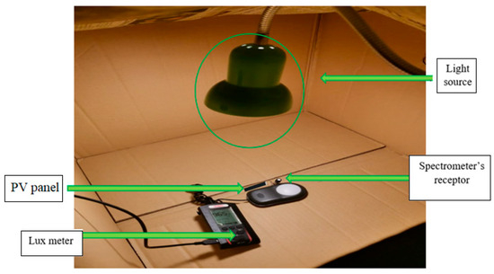
Figure 4.
Light source directly illuminating the spectrometer and lux meter.
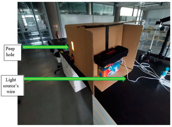
Figure 5.
Experimental setup in a confined box.
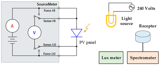
Figure 6.
Schematic diagram.
The light fixture is placed directly on top of the PV panel at a 90° angle, as shown in Figure 4, to obtain maximum performance. It is expected that if the angle is changed, the performance of the PV panels will be decreased [44]. A detailed investigation on how the angle of the light fixtures affects the performance of PV panels is an interesting direction that will be considered in future work.
The light spectra of the CFL and LED are shown in Figure 7 and Figure 8, respectively, in graphs generated using STELLARNET SpectraWiz software. The CFL spectrum is observed to have a narrower bandwidth and spikes at specific wavelengths, whereas the LED spectrum has a smoother distribution. The illuminance value presented in the upper-left corner can be derived by calculating the area under the curve within the wavelength range of 390–830 nm. This range is also referred to as the CIE 2008 photopic luminous efficiency function (E(λ)), which represents the average spectral sensitivity of human vision to light [45]. Thus, effective conversion would enable the use of a spectrometer to evaluate photovoltaic performance under low-illuminance conditions. The equation used to convert the measured spectral irradiance to spectral illuminance is expressed as [46]:
where V(λ) is the measured spectral irradiance value.
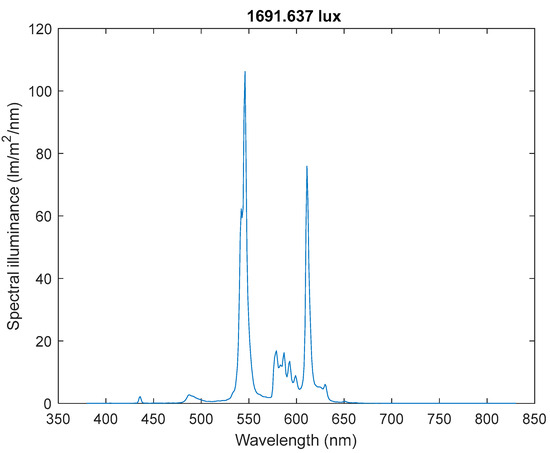
Figure 7.
12 W CFL spectrum.
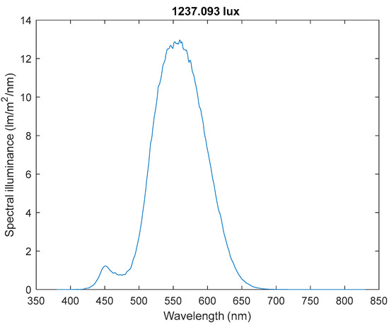
Figure 8.
7 W LED spectrum.
The 7 W LED and 12 W CFL light sources were chosen, since LED and CFL light sources outperform the other lights sources, such as xenon and incandescent lamps [47], in terms of efficiency. Therefore, their usage is expected to increase in the near future. The same methodology can also be used for any other light source.
The impact of different light sources and their respective spectra on conversion is mainly due to their efficiency, as most of their spectra fall within the wavelength range of 390–830 nm considered for illuminance. For example, Figure 7 and Figure 8 show that the power of the 12 W CFL is around 71% higher than that of the 7 W LED, but its illuminance is only 36% higher (1691.637 lux/1237.093 lux, respectively). This reflects the lower efficiency of CFL light when compared to LED light. Also, the values of 1691.637 lux and 1237.093 lux corresponds to 4.72 W/m2 and 4.05 W/m2, respectively.
For the experimental measurements, a total of 10 different illuminance levels are used to illuminate both PV panels (kx0b22−12x1 and kx0b22−04x3f). Illuminance levels range from 1000 lux to 100 lux with a 100 lux step size. To reduce measurement error, each illuminance level is measured 10 times, and the average is taken. As shown in Figure 9, a Keithley 2450 source measurement unit (SMU) is also used to record the panel’s I–V curve [48,49]. To eliminate the effects of lead resistance, a four-wire connection is established. The connections shown in Figure 6 are made as close as possible to the PV panel to avoid affecting the measurement accuracy due to the resistance of the probe cables. The results of the spectrometer and SMU are then exported to MATLAB to validate the proposed model’s accuracy.
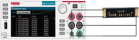
Figure 9.
SMU connection with the PV panel.
Both the characteristic point translation and parameter extraction techniques are implemented as MATLAB functions, which yield a set of model parameters for the corresponding PV panels depending on the measured reference values. During parameter extraction, the Rs value is increased at each iteration so that the maximum-power point of the corresponding I–V curve is as near as possible to the translated maximum-power point. Hence, it is expected that the sequence and combination of both the translation and parameter extraction techniques will be able to enhance the model’s accuracy.
The characteristics of the PV panels are given in Table 1. PV panel kx0b22−12x1 has one solar cell. On the other hand, kx0b22−04x3f consists of three solar cells. These three solar cells are connected in series. The solar cells used in both the PV panels are made of monocrystalline semiconductor material [50,51]. The table shows the PV panels’ STC datasheet values. However, the manufacturers did not provide the reference values under indoor illuminance conditions due to the low light intensity. Therefore, the experimental measurement at 1000 lux is used as the input values for the translation technique described in the previous section to translate the characteristic points to different illuminance levels.

Table 1.
Indoor PV panel datasheet values [50,51].
An overview of the experimental methodology and results is presented in Figure 10. The first and second steps are repeated for each artificial light source, whereas the third to fifth steps are repeated for each artificial light source and each PV panel.
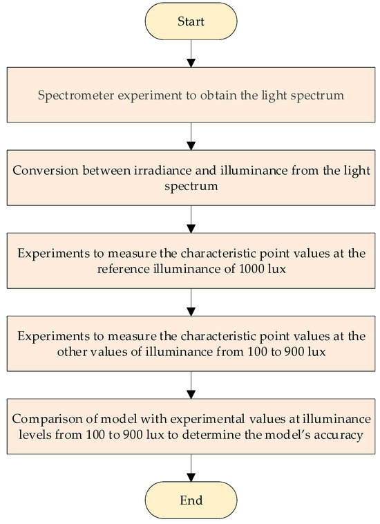
Figure 10.
Overview of the experimental methodology and results.
3. Results and Discussion
To determine the available energy at low illumination levels, a 1000 lux illuminance reference characteristic point value from the PV panels is used to translate to other illuminance levels. Both photovoltaic panels are exposed to 1000 lux with different light sources. The measured reference characteristic points are listed in Table 2 and Table 3.
Table 2.
Measured average reference characteristic points for kx0b22−12x1 at 1000 lux.
Table 3.
Measured average reference characteristic points for kx0b22−04x3f at 1000 lux.
Using the proposed translation technique, the reference values can be translated to different illuminance levels for various light sources. The model’s parameters can then be extracted with the translated characteristic point values as input values. Table 4 shows the extracted model’s parameter values at 1000 lux for one of the PV panels. It can be noted that the relatively higher value of Rs is due to the lower fill factor under indoor illumination.
Table 4.
Extracted parameters for kx0b22−12x1 at 1000 lux.
Bader [11] and Gandhi’s [16] works are used for comparison with the proposed model. This is because Bader improved the existing parameter extraction technique. Bader’s results appear promising, with low normalized root mean square deviation error (NRMSE) at low illumination levels. NRMSE is also applied to our proposed model in order to achieve the same benchmark for model accuracy. The NRMSE can be calculated using Equation (22):
where Iimod is the model’s value, Iiexp is the experimental value, and i is the value of a dataset of length k. On the other hand, Gandhi utilized the iterative thermal voltage to translate the open-circuit voltage, which is frequently employed in existing translation works. The same modeling procedures are applied to both panels at 900, 800, 700, 600 lux, etc. The values are recorded and compared to the experimental values.
The generated I–V curves are presented in Figure 11, Figure 12, Figure 13, Figure 14, Figure 15 and Figure 16. It can be noted that the values of the currents and voltages are very low due to the small size of the PV panels and the low illuminances of 1000 lux and below used in the experiments. For example, the current values in the data sheet [50,51] are in the order of mA, but these are provided for an irradiance level of 1000 W/m2, whereas 1000 lux is at least two orders of magnitude less, which results in current values in the order of µA. Figure 11 shows the I–V curves generated for both panels at 1000 lux; all of the I–V curves fit closely with the experimental values. As the illuminance level decreases, the accuracy of these works decreases. At 800 lux for the kx0b22−04x3f panel, the I–V curves near the maximum-power point begin to diverge. A similar situation also occurs at 600 lux, where the I–V curves for the kx0b22−04x3f panel differ, although still acceptable. However, Bader reported a slight overshoot after the maximum-power point for the kx0b22−12x1 panel.
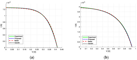
Figure 11.
Comparison of I–V curves obtained in different works with experimental values at 1000 lux with a 7 W LED: (a) kx0b22−12x1; (b) kx0b22−04x3f.
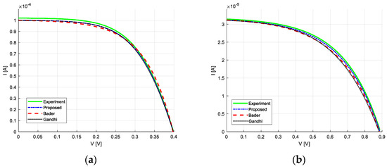
Figure 12.
Comparison of I–V curves obtained in different works with experimental values at 800 lux with a 7 W LED: (a) kx0b22−12x1; (b) kx0b22−04x3f.
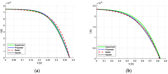
Figure 13.
Comparison of I–V curves obtained in different works with experimental values at 600 lux with a 7 W LED: (a) kx0b22−12x1; (b) kx0b22−04x3f.
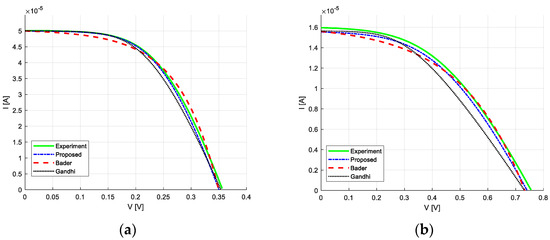
Figure 14.
Comparison of I–V curves obtained in different works with experimental values at 400 lux with a 7 W LED: (a) kx0b22−12x1; (b) kx0b22−04x3f.
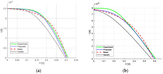
Figure 15.
Comparison of I–V curves obtained in different works with experimental values at 200 lux with a 7 W LED: (a) kx0b22−12x1; (b) kx0b22−04x3f.
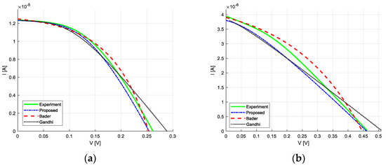
Figure 16.
Comparison of I–V curves obtained in different works with experimental values at 100 lux with a 7 W LED: (a) kx0b22−12x1; (b) kx0b22−04x3f.
At 400 lux, Bader overshot the I–V curve after the maximum-power point on both panels, with an additional undershoot before the maximum power point. On the other hand, the proposed model and Bader’s I–V curves do not differ much from the experimental values. Additionally, it can be clearly seen that Gandhi’s inaccurate translation of open-circuit voltage results in an undershoot for the kx0b22−04x3f panel’s I–V curve. Gandhi also encountered difficulties in translating the open-circuit voltage and maximum power voltage at 200 lux, as illustrated in Figure 15. Both of the I–V curves undershoot when compared to the experimental values. There is also a noticeable undershoot for Bader and the proposed model’s I–V curve near the kx0b22−04x3f panel’s short-circuit point. Due to the significant reduction in current at 100 lux, Gandhi struggled to accurately translate the open-circuit voltage, causing the I–V curve to overshoot after the maximum-power point. It can also be noted that the proposed model’s I–V curve undershoots the experimental values, while Bader’s I–V curve overshoots the maximum power point. Nevertheless, it remains within the acceptable range.
The results for the two PV panels (kx0b22−12x1 and kx0b22−04x3f) illuminated with a 7 W LED light source are presented in Table 5 and Table 6. At 1000 lux, the results of the discussed works fit very closely to the experimental values, resulting in a low NRMSE. However, the results indicate that as the illuminance level decreases, the NRMSE of both panels increases using all investigated methods. Bader’s NRMSE at 900 lux is 3.008%, which is slightly higher than that achieved with the other methods, while at 800 lux, Table 6 shows that Bader and Gandhi’s methods generated NRMSE values of 3.007% and 3.865%, respectively. Both results are more than two times that achieved with the proposed model (1.455%).
Table 5.
NRMSE of kx0b22−12x1 with a 7 W LED.
Table 6.
NRMSE of kx0b22−04x3f with a 7 W LED.
The NRMSE does not vary considerably between the investigated methods at 700 and 600 lux. However, the proposed model’s accuracy begins to outperform the other methods starting at 500 lux. At this level, Gandhi’s method generates an NRMSE of 6.145% (Table 5). This is due to the use of iterative thermal voltage to translate the open-circuit voltage. The iterative process is unable to provide an accurate fit for low-wattage panels with a low number of PV cells. As the thermal voltage is used in the subsequent translation, it affects the model’s accuracy. In comparison, the proposed model provides a significantly lower NRMSE of 2.258%. This is because the proposed translated open-circuit voltage is derived from the relationship between light and voltage using all three characteristic points. Hence, the model’s accuracy can be improved. Gandhi’s method also encounters difficulties in accurately modeling the maximum-power voltage at 400 and 300 lux, resulting in NRMSE values of 7.993% and 8.619%, respectively. Although Gandhi’s initial series resistor serves to represent PV losses under outdoor conditions, the assumption of an infinite value of Rp in the derivation affects its accuracy considerably under indoor conditions. It can be seen that at 200 lux, Gandhi‘s NRMSE values are significantly higher for both panels (11.709% and 11.170%) due to inaccurate translation. Bader’s NRMSE has slowly increase to 4.935% at the same illuminance level. As Bader’s method improves the existing parameter extraction technique, its associated NRMSE value is not as high as that of Gandhi’s method. However, Bader’s still involves the use of the parameter-scaling technique, which degrades at low illuminance levels. Most of the investigated methods are unable to maintain their accuracy at 100 lux. As shown in Table 6, the Bader method and the proposed model generate accuracies of 5.488% and 5.513%, respectively. Gandhi’s method also fails to maintain its accuracy on both panels, resulting in NRMSE values of 14.703% and 12.051%.
In summary, the proposed model provides average NRMSE values of 2.171% and 2.691%, corresponding to a 17.149% to 19.712% improvement over Bader’s method. The proposed model is able to achieve this by combining the best features of Wahed’s [14] translation technique and Fahad’s parameter extraction technique [12]. The improved accuracy of the proposed model over the compared methods highlights its importance and contribution.
Figure 17, Figure 18 and Figure 19 show the I–V curves of both panels at 1000, 800, and 600 lux under 12 W CFL illumination, respectively. The results are very similar to those presented in Figure 11, Figure 12 and Figure 13. This is because the PV panels are illuminated by a similar level of light intensity, and the experimental range of the light spectrum has little effect on PV absorption. As the illuminance level decreases, the accuracy of these methods starts to decrease. At 400 lux, the Bader method continues to undershoot the I–V curve after the short-circuit point on both panels. On the other hand, the I–V curves of the proposed model and those associated with Bader’s method do not differ much from the experimental values.
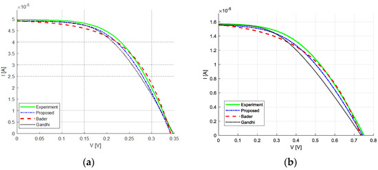
Figure 17.
Comparison of I–V curves obtained in different works with experimental values at 400 lux with a 12 W CFL: (a) kx0b22−12x1; (b) kx0b22−04x3f.
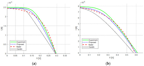
Figure 18.
Comparison of I–V curves obtained in different works with experimental values at 200 lux with a 12 W CFL: (a) kx0b22−12x1; (b) kx0b22−04x3f.
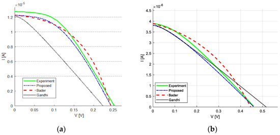
Figure 19.
Comparison of I–V curves obtained in different works with experimental values at 100 lux with a 12 W CFL: (a) kx0b22−12x1; (b) kx0b22−04x3f.
At 200 lux, Gandhi’s method results in inaccurate translation of the maximum-power voltage and open-circuit voltage, as illustrated in Figure 18. Bader’s method results in a noticeable undershoot of the I–V curves near the kx0b22−12x1 panel’s short-circuit point, which is also reflected by the high NRMSE. Hence, both of the I–V curves result in an undershoot compared with the experimental values. Due to the significant reduction in current at 100 lux, Gandhi’s method struggles to accurately translate the open-circuit voltage, causing the I–V curve to be overshot after the maximum-power point. It can also be noted that the proposed model’s I–V curve undershoots the experimental values, while Bader’s I–V curve overshoots the maximum-power point.
Table 7 and Table 8 show the corresponding NRMSE results for both panels when illuminated by a 12 W CFL light source. At 1000 lux, the discussed methods fit the experimental values very closely, resulting in a low NRMSE. Between 900 and 600 lux, the performance of all three methods is similar. Nevertheless, as seen in Table 7, Gandhi’s method results in a slightly higher NRMSE of 3.261% at 700 lux, which is more than twice that of the other methods. Gandhi’s method is also associated with NRMSE values of 6.057%, 4.529%, and 8.385% at 500, 400, and 300 lux, respectively. This is because the translation of the maximum-power voltage is inaccurate, resulting in an increase in the NRMSE. Furthermore, at 200 lux, Gandhi’s method also struggles to translate the open-circuit voltage due to the iterative thermal voltage. The results show that NRMSE values obtained with Gandhi’s method reached as high as 14.123%. At 100 lux, the majority of the investigated methods struggle to maintain their accuracy. Due to the inaccuracy of the translation technique, Gandhi’s method has the highest NRMSE of 28.086%. Since Bader’s method involves the use of the parameter-scaling technique, the NRMSE rises to 6.070%. Nonetheless, the proposed model also had issues at 100 lux, with an NRMSE of 4.269%. It is important to note that potential nonlinearities can occur in the I–V curve, especially under varying indoor conditions. Nevertheless, the two existing techniques used in this study already have an inherent capability to handle potential nonlinearities in the I–V curve. Additionally, the iterative approach was applied in this study, which adjusts the Rs value to handle nonlinearities.
Table 7.
NRMSE of kx0b22−12x1 with a 12 W CFL.
Table 8.
NRMSE of kx0b22−04x3f with a 12 W CFL.
In summary, the results show that the proposed model can provide average NRMSE values of 2.463% and 2.857%, which is a 13.029% to 13.091% improvement over the values achieved with Bader’s method. Based on the discussion of the performance achieved with the other investigated methods, it can be concluded that Gandhi’s method struggles to accurately translate open-circuit voltage due to the iterative thermal voltage and that the assumption of an infinite Rp value causes a lack of accuracy in maximum-power voltage translation at low illuminance levels. Moreover, Bader’s parameter-scaling technique is unable to generate an accurate and consistent I–V curve. The proposed model is shown to provide the best accuracy among these works, with an average improvement of 15.75%. This is because the proposed model adopts the best features of both techniques, i.e., characteristic point translation followed by parameter extraction and an iterative adjustment of Rs to match the lower maximum-power point at low illuminance levels.
4. Conclusions
The use of PV panels to convert light into electricity in indoor environments is expected to increase significantly in tandem with the rapid deployment of low-power IoT sensor devices. Hence, an accurate model is required to evaluate and predict the performance of PV panels. However, the nonlinear characteristics of PV panels make the modeling of their electrical response a challenging task. In this paper, we present a one-diode PV model with two resistors with improved characteristic point translation and parameter extraction techniques for indoor PV modeling. This model only requires one set of reference values, such as those at 1000 lux, to predict the electrical behavior of PV panels under different illuminance levels, which enables its wide applicability. Two PV panels were used and illuminated under different types of commonly employed light technologies. The model was tested, and its results were compared to those reported in other works using parameter-scaling and translation techniques, in addition to comparison with experimental values. The results show that the proposed model’s accuracy is higher than that of the compared methods and close to the experimental values. Furthermore, the proposed model is able to provide an average accuracy improvement of 15.75% over the compared methods. Therefore, the proposed model, which can provide consistently high accuracy in modeling PV behavior at various illuminance levels for different light and PV technologies, can contribute to the explosive growth in the development of new energy for sustainable indoor IoT applications.
There are many interesting possible directions for future work. First, the investigation of the effects of temperature and its modeling is an exciting proposition that can extend the model’s applicability. Secondly, how the angle between the light source and the PV panel affects the performance of the latter is another worthwhile direction for future research. Lastly, the extension of the model to other light sources and emerging PV technologies, especially for indoor applications, will be studied in the future.
Author Contributions
Conceptualization, C.J.Q.T. and M.D.; methodology, C.J.Q.T. and M.D.; validation, M.D. and R.A.; formal analysis, C.J.Q.T. and M.D.; investigation, C.J.Q.T.; resources, K.N.M.H.; writing—original draft preparation, C.J.Q.T.; writing—review and editing, M.D., K.N.M.H., A.L.S., and R.A.; visualization, A.L.S.; supervision, M.D.; funding acquisition, K.N.M.H. All authors have read and agreed to the published version of the manuscript.
Funding
This research was funded (APC) by Yayasan Universiti Teknologi PETRONAS YUTP-FRG 1/2021: 015LC0-349.
Data Availability Statement
Data are contained within the article.
Acknowledgments
The authors gratefully acknowledge the support of this research from Universiti Teknologi PETRONAS.
Conflicts of Interest
The authors declare no conflict of interest.
References
- Garaj, M.; Chung, H.S.-H.; Spataru, S.; Lo, A.W.-L.; Wang, H. A granular modeling method for non-uniform panel degradation based on I–V characterization and electroluminescence imaging. Sol. Energy 2021, 227, 162–178. [Google Scholar] [CrossRef]
- Sayed, E.A.; Sameh, M.A.; Attia, M.A.; Badr, A.O. Enhancement of PV performance by using hybrid TLBO-EO optimization. Ain Shams Eng. J. 2023, 14, 101892. [Google Scholar] [CrossRef]
- Adouairi, M.S.; Bossoufi, B.; Motahhir, S.; Saady, I. Application of fuzzy sliding mode control on a single-stage grid-connected PV system based on the voltage-oriented control strategy. Results Eng. 2023, 17, 100822. [Google Scholar] [CrossRef]
- Teh, C.J.; Drieberg, M.; Soeung, S.; Ahmad, R. Simple PV modeling under variable operating conditions. IEEE Access 2021, 9, 96546–96558. [Google Scholar] [CrossRef]
- Politi, B.; Foucaran, A.; Camara, N. Low-cost sensors for indoor pv energy harvesting estimation based on machine learning. Energies 2022, 15, 1144. [Google Scholar] [CrossRef]
- Memon, Z.A.; Akbari, M.A.; Zare, M. An improved cheetah optimizer for accurate and reliable estimation of unknown parameters in photovoltaic cell and module models. Appl. Sci. 2023, 13, 9997. [Google Scholar] [CrossRef]
- Soliman, M.A.; Hasanien, H.M.; Alkuhayli, A. Marine predators algorithm for parameters identification of triple-diode photovoltaic models. IEEE Access 2020, 8, 155832–155842. [Google Scholar] [CrossRef]
- Duan, Z.; Yu, H.; Zhang, Q.; Tian, L. Parameter extraction of solar photovoltaic model based on nutcracker optimization algorithm. Appl. Sci. 2023, 13, 6710. [Google Scholar] [CrossRef]
- Ma, X.; Bader, S.; Oelmann, B. A scalable, data-driven approach for power estimation of photovoltaic devices under indoor conditions. In Proceedings of the 7th International Workshop on Energy Harvesting & Energy-Neutral Sensing Systems, New York, NY, USA, 10 November 2019; pp. 29–34. [Google Scholar]
- Ma, X.; Bader, S.; Oelmann, B. On the performance of the two-diode model for photovoltaic cells under indoor artificial lighting. IEEE Access 2020, 9, 1350–1361. [Google Scholar] [CrossRef]
- Bader, S.; Ma, X.; Oelmann, B. A Comparison of One-and Two-Diode Model Parameters at Indoor Illumination Levels. IEEE Access 2020, 8, 172057–172064. [Google Scholar] [CrossRef]
- Rasool, F.; Drieberg, M.; Badruddin, N.; Singh, B.S.M. PV panel modelling with improved parameter extraction technique. Sol. Energy 2017, 153, 519–530. [Google Scholar] [CrossRef]
- Bader, S.; Ma, X.; Oelmann, B. One-diode photovoltaic model parameters at indoor illumination levels—A comparison. Sol. Energy 2019, 180, 707–716. [Google Scholar] [CrossRef]
- Abd Al-Wahed, M.E.; Abdullateef, O.F. Modeling of monocrystalline PV cell considering ambient conditions in Baghdad city. Al-Khwarizmi Eng. J. 2017, 13, 74–82. [Google Scholar] [CrossRef][Green Version]
- Elyaqouti, M.; Saadaoui, D.; Lidaighbi, S.; Chaoufi, J.; Ibrahim, A.; Aqel, R.; Obukhov, S. A novel hybrid numerical with analytical approach for parameter extraction of photovoltaic modules. Energy Convers. Manag. X 2022, 14, 100219. [Google Scholar]
- Gandhi, O.; Rodríguez-Gallegos, C.D.; Gorla, N.B.Y.; Bieri, M.; Reindl, T.; Srinivasan, D. Reactive power cost from PV inverters considering inverter lifetime assessment. IEEE Trans. Sustain. Energy 2018, 10, 738–747. [Google Scholar] [CrossRef]
- Batzelis, E.I.; Papathanassiou, S.A. A method for the analytical extraction of the single-diode PV model parameters. IEEE Trans. Sustain. Energy 2015, 7, 504–512. [Google Scholar] [CrossRef]
- Batzelis, E.I. Simple PV performance equations theoretically well founded on the single-diode model. IEEE J. Photovolt. 2017, 7, 1400–1409. [Google Scholar] [CrossRef]
- El-Khozondar, H.J.; Yen, J.T.W.; Koch, A.W. Simulating the performance and output measurements of modeled Photovoltaic (PV) Inverter. In Proceedings of the 7th IEEE Palestinian International Conference on Electrical and Computer Engineering (PICECE), Gaza, Palestine, 26–27 March 2019; pp. 1–6. [Google Scholar]
- Bayarassou, H.; Megri, A.F. New approach based on a fuzzy regression model for a photovoltaic system. Electr. Power Syst. Res. 2023, 217, 109091. [Google Scholar] [CrossRef]
- Fang, Z.; Lin, Y.; Song, S.; Song, C.; Lin, X.; Cheng, G. Active distribution system state estimation incorporating photovoltaic generation system model. Electr. Power Syst. Res. 2020, 182, 106247. [Google Scholar] [CrossRef]
- Drouiche, I.; Harrouni, S.; Arab, A.H. A new approach for modelling the aging PV module upon experimental I–V curves by combining translation method and five-parameters model. Electr. Power Syst. Res. 2018, 163, 231–241. [Google Scholar] [CrossRef]
- Hassan, O.; Zakzouk, N.; Abdelsalam, A. Novel photovoltaic empirical mathematical model based on function representation of captured figures from commercial panels datasheet. Mathematics 2022, 10, 476. [Google Scholar] [CrossRef]
- Sarniak, M.T. Modeling the functioning of the half-cells photovoltaic module under partial shading in the matlab package. Appl. Sci. 2020, 10, 2575. [Google Scholar] [CrossRef]
- Bayoumi, A.S.; El-Sehiemy, R.A.; Mahmoud, K.; Lehtonen, M.; Darwish, M.M. Assessment of an improved three-diode against modified two-diode patterns of MCS solar cells associated with soft parameter estimation paradigms. Appl. Sci. 2021, 11, 1055. [Google Scholar] [CrossRef]
- Al-Ezzi, A.S.; Ansari, M.N.M. Photovoltaic solar cells: A review. Appl. Syst. Innov. 2022, 5, 67. [Google Scholar] [CrossRef]
- Bo, Q.; Cheng, W.; Khishe, M.; Mohammadi, M.; Mohammed, A.H. Solar photovoltaic model parameter identification using robust niching chimp optimization. Sol. Energy 2022, 239, 179–197. [Google Scholar] [CrossRef]
- Manuel Godinho Rodrigues, E.; Godina, R.; Marzband, M.; Pouresmaeil, E. Simulation and comparison of mathematical models of PV cells with growing levels of complexity. Energies 2018, 11, 2902. [Google Scholar] [CrossRef]
- Danandeh, M.A.; Mousavi G, S.M. Comparative and comprehensive review of maximum power point tracking methods for PV cells. Renew. Sustain. Energy Rev. 2018, 82, 2743–2767. [Google Scholar] [CrossRef]
- Batarseh, M.G.; Za’ter, M.E. Hybrid maximum power point tracking techniques: A comparative survey, suggested classification and uninvestigated combinations. Sol. Energy 2018, 169, 535–555. [Google Scholar] [CrossRef]
- Mathew, L.E.; Panchal, A.K. A complete numerical investigation on implicit and explicit PV single-diode-models using I-and V-approaches. IEEE J. Photovolt. 2021, 11, 827–837. [Google Scholar] [CrossRef]
- Khezzar, R.; Zereg, M.; Khezzar, A. Modeling improvement of the four parameter model for photovoltaic modules. Sol. Energy 2014, 110, 452–462. [Google Scholar] [CrossRef]
- Nafil, R.Q.; Khamees, H.T.; Majeed, M.S. Identification the internal parameters for mono-crystalline solar module using Matlab-simulation and experimental ascertainment. TELKOMNIKA Telecommun. Comput. Electron. Control. 2021, 19, 716–723. [Google Scholar] [CrossRef]
- Polo, J.; Martín-Chivelet, N.; Alonso-García, M.C.; Zitouni, H.; Alonso-Abella, M.; Sanz-Saiz, C.; Vela-Barrionuevo, N. Modeling IV curves of photovoltaic modules at indoor and outdoor conditions by using the Lambert function. Energy Convers. Manag. 2019, 195, 1004–1011. [Google Scholar] [CrossRef]
- Jenkal, S.; Kourchi, M.; Rachdy, A.; Oussalem, O.; Ajaamoum, M.; Oubella, M. Modeling a Photovoltaic Emulator Using Four Methods and Buck-Boost Converter. Eng. Lett. 2021, 29, 1–8. [Google Scholar]
- Vergura, S. A complete and simplified datasheet-based model of pv cells in variable environmental conditions for circuit simulation. Energies 2016, 9, 326. [Google Scholar] [CrossRef]
- Anderson, A. Photovoltaic Translation Equations: A New Approach. Final Subcontract Report; National Renewable Energy Lab. (NREL): Golden, CO, USA, 1996. Available online: https://www.nrel.gov/docs/legosti/old/20279.pdf (accessed on 2 May 2023).
- Müller, M.; Wienold, J.; Walker, W.D.; Reindl, L.M. Characterization of indoor photovoltaic devices and light. In Proceedings of the 34th IEEE Photovoltaic Specialists Conference (PVSC), Philadelphia, PA, USA, 7–12 June 2009; pp. 738–743. [Google Scholar]
- Fontana, L. Effect of indoor surfaces’ spectral reflectance on the environmental light spectrum modification and on objects perceived color. Results Eng. 2023, 17, 100805. [Google Scholar] [CrossRef]
- 7W E27 Cap White Bulb, Philips. Available online: https://www.lighting.philips.com.my/consumer/p/led-bulb/8718696845332 (accessed on 16 January 2023).
- Tornado 12W CDL E27 220-240V 1PF/6, Philips. Available online: https://www.lighting.philips.com/main/prof/conventional-lamps-and-tubes/compact-fluorescent-integrated/energy-saver-twister-shape/tornado-t2/929689868601_EU/product (accessed on 16 January 2023).
- Apostolou, G.; Verwaal, M.; Reinders, A. Estimating the performance of product integrated photovoltaic (PIPV) cells under indoor conditions for the support of design processes. In Proceedings of the 40th IEEE Photovoltaic Specialist Conference (PVSC), Denver, CO, USA, 8–13 June 2014; pp. 742–747. [Google Scholar]
- Masoudinejad, M.; Emmerich, J.; Kossmann, D.; Riesner, A.; Roidl, M.; ten Hompel, M. Development of a measurement platform for indoor photovoltaic energy harvesting in materials handling applications. In Proceedings of the IREC2015 The Sixth International Renewable Energy Congress, Sousse, Tunisia, 24–26 March 2015; pp. 1–6. [Google Scholar]
- Mamun, M.; Islam, M.; Hasanuzzaman, M.; Selvaraj, J. Effect of tilt angle on the performance and electrical parameters of a PV module: Comparative indoor and outdoor experimental investigation. Energy Built Environ. 2022, 3, 278–290. [Google Scholar] [CrossRef]
- Li, H.-C.; Sun, P.-L.; Huang, Y.; Luo, M.R. Spectral optimization of white LED based on mesopic luminance and color gamut volume for dim lighting conditions. Appl. Sci. 2020, 10, 3579. [Google Scholar] [CrossRef]
- Michael, P.R.; Johnston, D.E.; Moreno, W. A conversion guide: Solar irradiance and lux illuminance. J. Meas. Eng. 2020, 8, 153–166. [Google Scholar] [CrossRef]
- de Souza, D.F.; da Silva, P.P.F.; Fontenele, L.F.A.; Barbosa, G.D.; de Oliveira Jesus, M. Efficiency, quality, and environmental impacts: A comparative study of residential artificial lighting. Energy Rep. 2019, 5, 409–424. [Google Scholar] [CrossRef]
- Reynaud, C.A.; Clerc, R.; Lechene, P.B.; Hebert, M.; Cazier, A.; Arias, A.C. Evaluation of indoor photovoltaic power production under directional and diffuse lighting conditions. Sol. Energy Mater. Sol. Cells 2019, 200, 110010. [Google Scholar] [CrossRef]
- Aoki, Y. Photovoltaic performance of Organic Photovoltaics for indoor energy harvester. Org. Electron. 2017, 48, 194–197. [Google Scholar] [CrossRef]
- KXOB22-04X3F: Digi-Key Electronics, DigiKey. Available online: https://www.digikey.com/en/products/detail/anysolar-ltd/KXOB22-04X3F/4840080 (accessed on 17 April 2023).
- KXOB22-12X1: Digi-Key Electronics, DigiKey. Available online: https://www.digikey.com/en/products/detail/anysolar-ltd/KXOB22-12X1/2754272 (accessed on 17 April 2023).
Disclaimer/Publisher’s Note: The statements, opinions and data contained in all publications are solely those of the individual author(s) and contributor(s) and not of MDPI and/or the editor(s). MDPI and/or the editor(s) disclaim responsibility for any injury to people or property resulting from any ideas, methods, instructions or products referred to in the content. |
© 2024 by the authors. Licensee MDPI, Basel, Switzerland. This article is an open access article distributed under the terms and conditions of the Creative Commons Attribution (CC BY) license (https://creativecommons.org/licenses/by/4.0/).