

Analysis of Adaptive Individual Pitch Control Schemes for Blade Fatigue Load Reduction on a 15 MW Wind Turbine

 ,
, 
 and
and 
Abstract
:1. Introduction
- In closely related previous research [14], IPC schemes with two identical pure integral controllers with and without the azimuth offset were compared. In this work, a study in more detail is performed for simple IPC schemes optimized to minimize the fatigue blade load. Specifically, we check the influence of using integral or proportional controllers, tuning them with different gains and including or not including the azimuth offset in the reverse MBC transform. The improvements that can be achieved considering these features are analyzed qualitatively and quantitatively.
- The IPC schemes are implemented as adaptive blocks where the controller gains are scheduled according to the mean value of the measured filtered blade moments instead of the wind speed in the above-rated region.
- Most of the research papers published so far on OpenFAST have concentrated on the 5 MW NREL turbine. However, this study is conducted on a 15 MW turbine, a type of turbine on which not much research has been conducted so far.
2. MBC Transform
3. Proposed Methodology
3.1. Wind Turbine Model and Simulation Framework
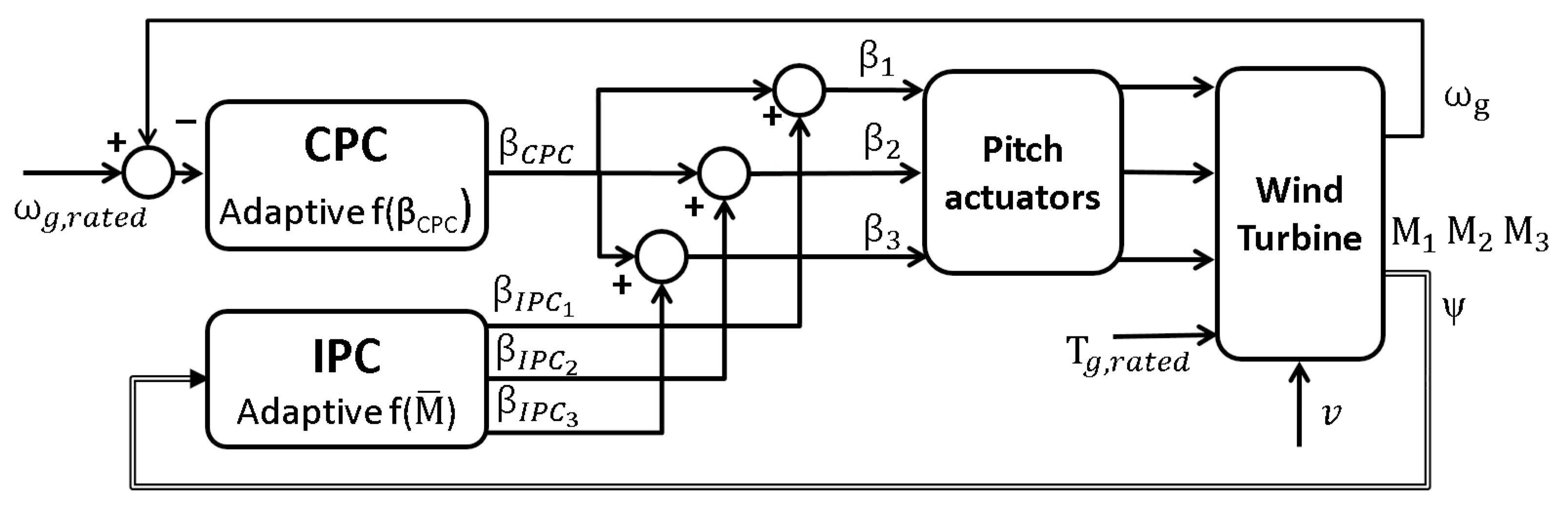
3.2. Control System Scheme
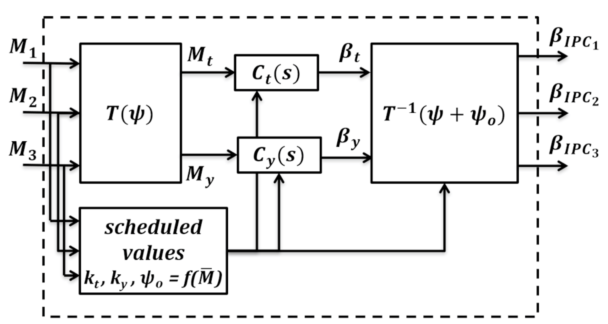
- Control 1 (IPC_P2): The IPC comprises two different P controllers, and no azimuth offset is tuned. Therefore, Ct(s) = Cy(s) = 1, kt ≠ ky, and ψo = 0°. There are only two parameters to be tuned: the controller gains.
- Control 2 (IPC_P2ψ): The IPC comprises two different P controllers and includes the azimuth offset. Therefore, Ct(s) = Cy(s) = 1 and kt ≠ ky. There are three parameters to be tuned: the controller gains kt and ky and the azimuth offset ψo.
- Control 3 (IPC_I1): The IPC is composed of two identical I controllers because they are forced to have the same gain; no azimuth offset is tuned. Therefore, Ct(s) = Cy(s) = 1/s, kt = ky, and ψo = 0°. There is only one parameter to be tuned: the common controller gain.
- Control 4 (IPC_I1ψ): The IPC is composed of two identical I controllers and includes the azimuth offset. Therefore, Ct(s) = Cy(s) = 1/s and kt = ky. There are two parameters to be tuned: the common controller gain and the azimuth offset ψo.
- Control 5 (IPC_I2): The IPC comprises two different I controllers, and no azimuth offset is tuned. Therefore, Ct(s) = Cy(s) = 1/s, kt ≠ ky, and ψo = 0°. There are two tuning parameters: the controller gains.
- Control 6 (IPC_I2ψ): The IPC comprises two different I controllers and includes the azimuth offset. Therefore, Ct(s) = Cy(s) = 1/s and kt ≠ ky. There are three parameters to be tuned: the controller gains and the azimuth offset ψo.
3.3. IPC Tuning by Optimization
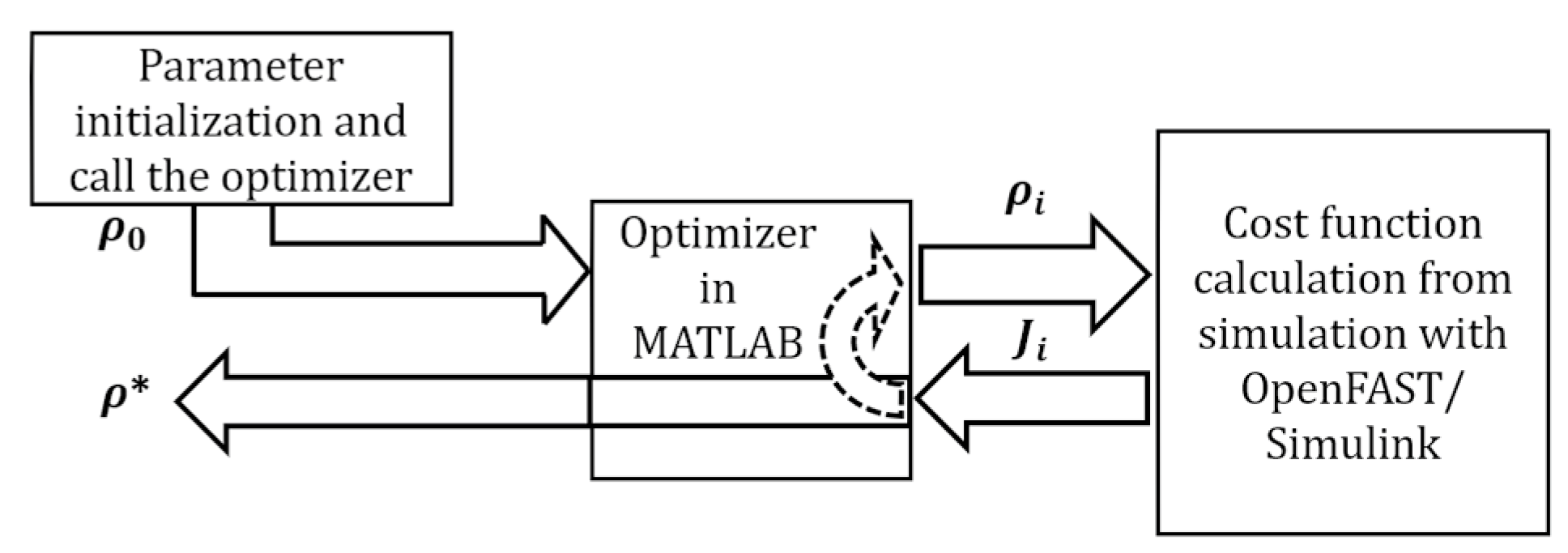
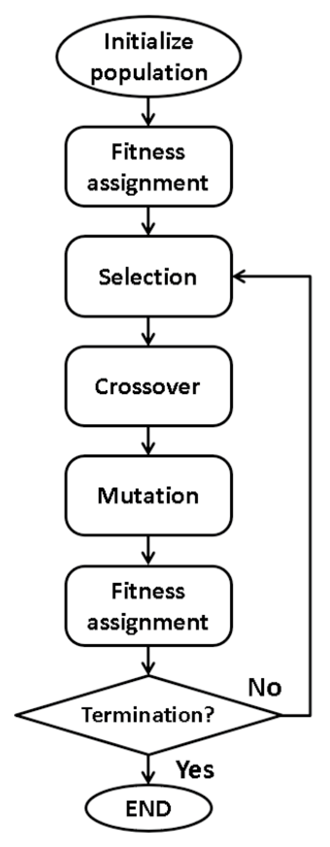
3.4. Optimization Algorithm
- Initial population: Before optimization, the tuning parameter search range is set manually using a bisection-type procedure, where the range is reduced by eliminating parameter values that cause instability during simulation. The search interval for the gains is [0–0.3] deg/(MN·m·s) for integral controllers or [0–2] deg/(MN·m) for proportional controllers, and the range for the azimuth offset is [0–90] deg. An initial population of 100 individuals is created with parameter values evenly spaced within the defined range; the population size is 200 for the IPC cases with three parameters to be tuned.
- Fitness assignment: After initialization, every individual in the population or chromosome is assigned a fitness value. When using a simulation-based approach, the fitness value of each member is calculated by running a simulation. The fitness function is equivalent to the cost function J being optimized.
- Selection: Its purpose is to select the most suitable individuals and pass on their genes to the following generation. This study uses the roulette selection method, which assigns a higher probability of fitness to chromosomes with lower fitness values, making them more likely to be chosen. The fitness probability of the i-th individual is represented by Pi = Ji/ and its corresponding cumulative fitness probability qi = . Subsequently, a selection is made by considering the previous probability value’s position in the roulette, represented on a cumulative probability of suitability scale. For this purpose, a pseudo-random number r uniformly distributed over the interval [0, 1] is generated. If qk−1 ≤ r ≤ qk, then the k-th candidate is chosen as a parent. In order to reach the required number of parents, the number r is generated multiple times. The best chromosomes are always retained in the population (elite selection). The number of elite individuals in the population is set to 0.05 times the population size.
- Crossover: This operator creates part of a new population by recombining the selected individuals after sorting and rejecting the chromosomes. For each parent couple (mum and dad), defined in Equation (7), a random gene-crossing point, defined by the random variable α, is chosen before mating. The mom and dad are denoted by subscripts m and d, respectively. The selected parameters pm,α and pd,α are grouped according to Equation (8) to generate new values, pnew1 and pnew2, which appear in the descendants. The parameter γ is a random number within the range of [0, 1]. Then, as shown in Equation (9), the mating process is completed by exchanging other genes (parameters) and obtaining offspring. The crossover fraction is set to 0.75, which represents the fraction of the population created by this operator.
- 5.
- Mutation: Transfer a small amount of randomness to new individuals to maintain diversity within the population and avoid locally optimal tracking such as crossover. The mutation probability is set to 0.2.
- 6.
- New individual generation: The process of genetic recombination involves the creation of new populations by recombining the resultant offspring with other mutated offspring. This process is repeated until the termination condition is met. This process stops when the fitness of a particular solution achieves the desired level of fitness, the number of generations reaches a maximum limit, or the population becomes stable. In this work, after reaching 20 generations without changes in the best fitness, the process stops because it has been observed that this number is sufficient for convergence in the proposed optimization.
4. Results and Discussion
4.1. Optimization Results
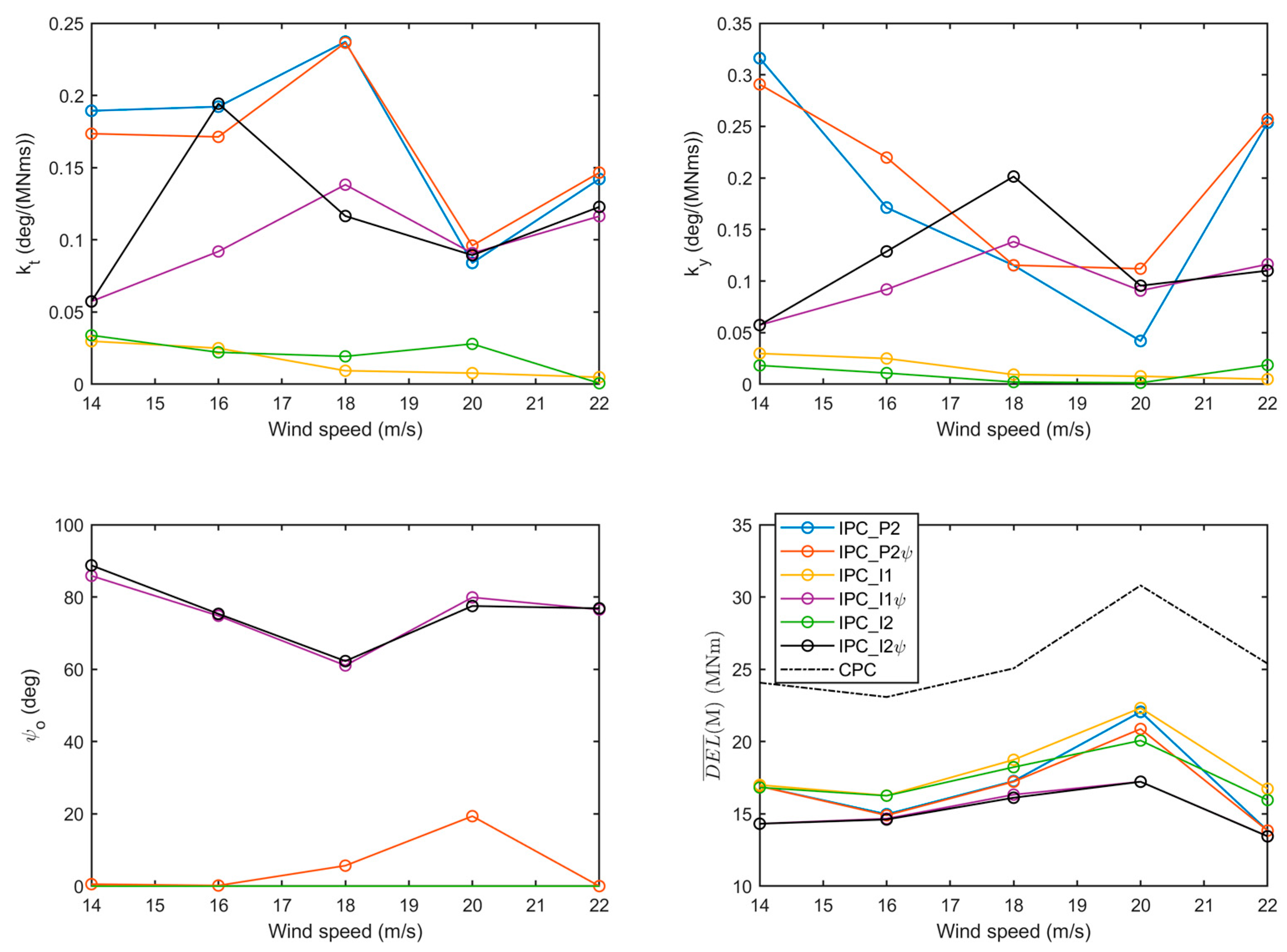
- The IPC schemes with integral controllers plus the azimuth offset (IPC_I1ψ and IPC_I2ψ) achieved the largest reductions in the mean DEL value at all operating points evaluated. The average reduction was 41% with respect to the CPC case. The third best scheme was the IPC with P controllers and the azimuth offset (IPC_P2ψ), which showed an average reduction of 35% in the mean DEL value.
- The IPC schemes with integral action and without the azimuth offset showed the lowest gains and the lowest DEL reductions—only 30% on average. Including the azimuth offset in these schemes allowed the optimal designs to achieve higher gains.
- The two IPC schemes with integral controllers and the azimuth offset (IPC_I1ψ and IPC_I2ψ) had practically the same azimuth offset values ψo at each operation point. In the IPC scheme with proportional controllers plus the azimuth offset (IPC_P2ψ), the values of ψo were practically zero at all operation points except at 20 m/s. Even so, there did not seem to be much effect on the results when it was set to zero. This is because the integral action adds phase delay, whereas the proportional action does not.
- On the contrary, if we compare the IPC cases with integral controllers, the inclusion of the azimuth offset allowed an increase in the average DEL reduction of the OoP blade moments of about 10% more compared to the same scheme without the offset. Schemes IPC_I1 and IPC_I2 had an average DEL reduction of approximately 30%, but their respective cases with the azimuth offset (IPC_I1ψ and IPC_I2ψ) had an average reduction of 41%.
- Of the two best IPC schemes (IPC_I1ψ and IPC_I2ψ), the IPC_I1ψ case could be considered the most advisable, because, having achieved similar results, it had only two parameters to adjust. It does not seem worthwhile to let the integral gains be different (case IPCI2_ψ) since it does not provide significant improvements and requires the three parameters to be tuned. Furthermore, it was observed that the gains of both kt and ky were practically the same at several operating points.
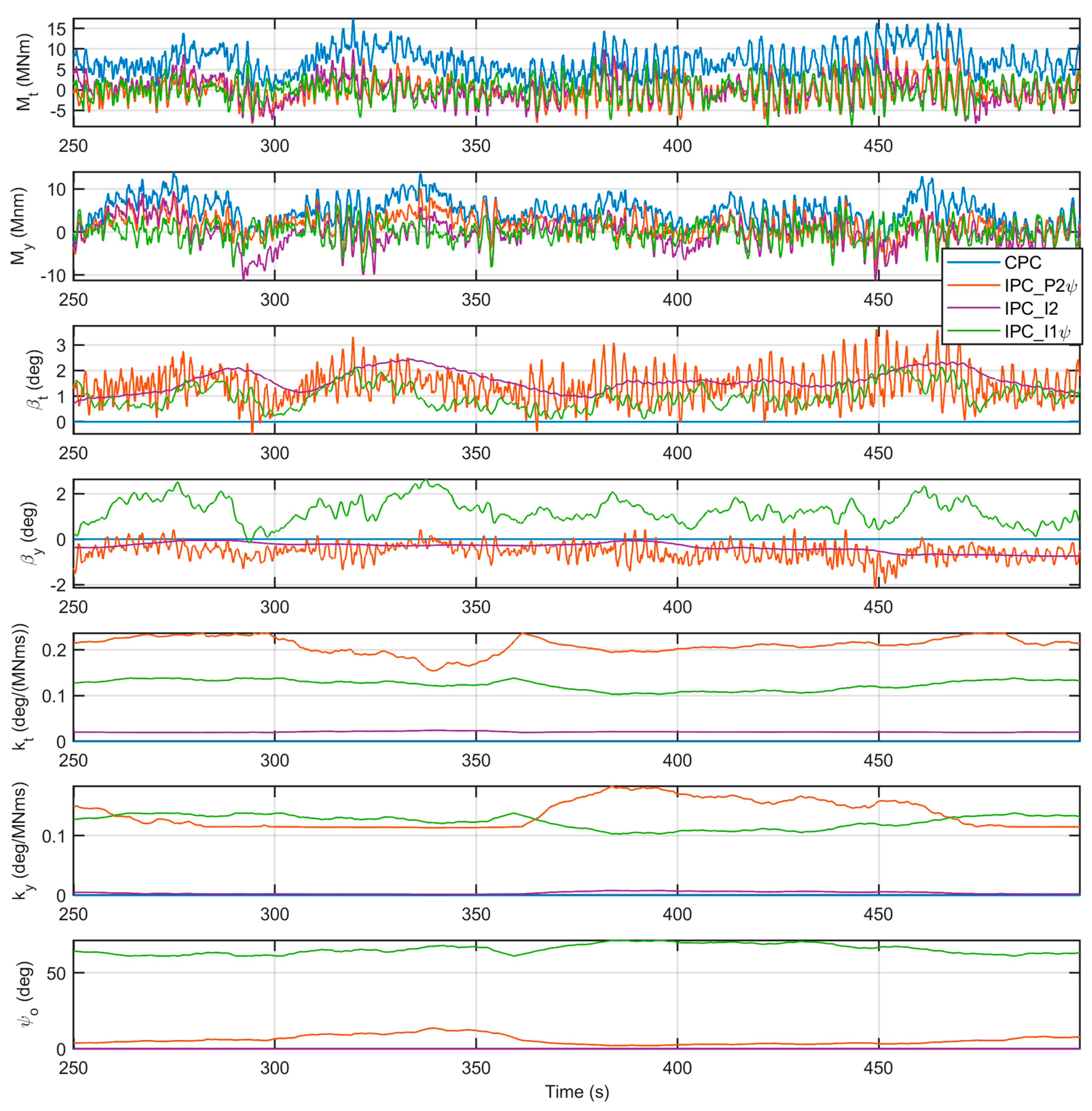
4.2. Simulation Results in the Rotating Reference Frame
4.3. Simulation Results in the Non-Rotating Reference Frame
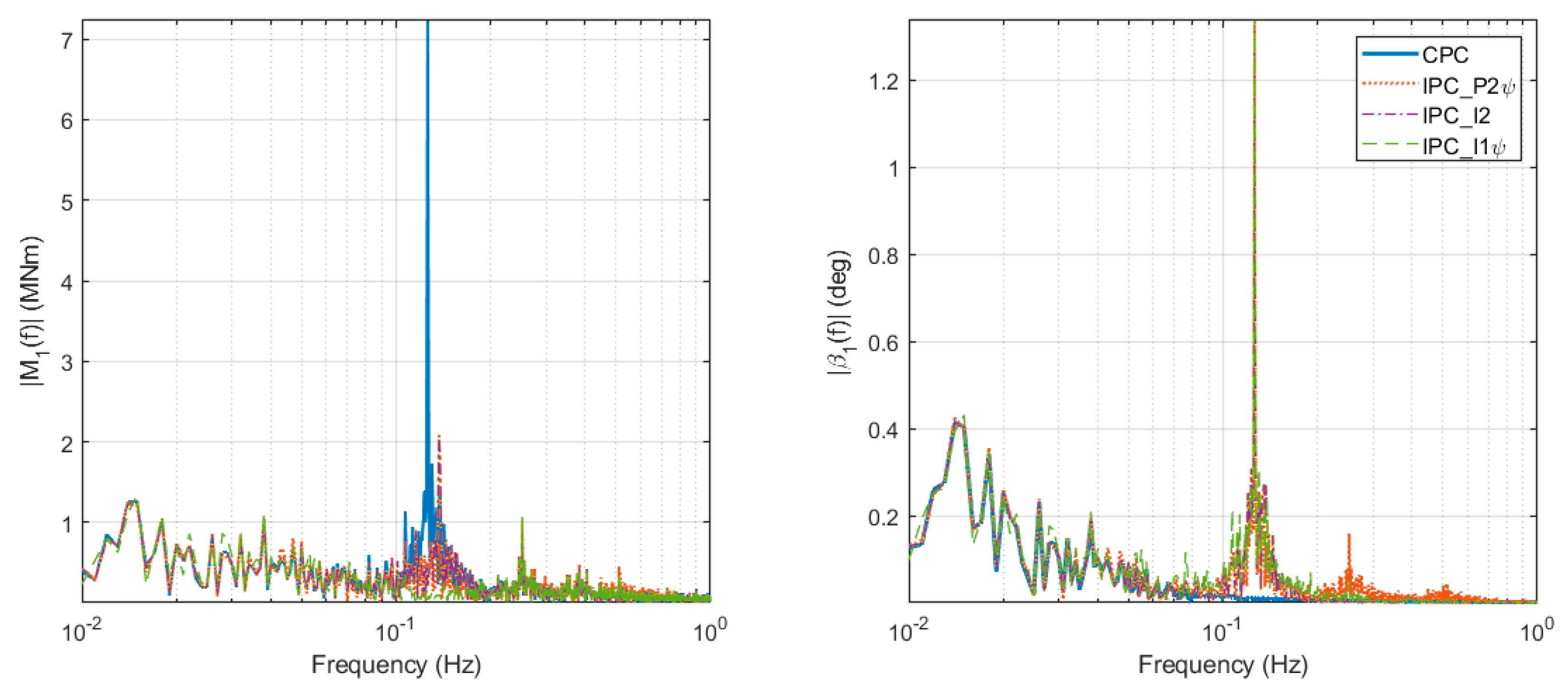
4.4. Frequency Response
5. Conclusions
- The optimal IPC solution with proportional controllers (with or without the azimuth offset) produces a similar reduction in DEL values as the optimal solution of IPC with integral controllers without the azimuth offset; however, the proportional controllers produce higher pitch signal activity.
- The IPC schemes with integral controllers and the azimuth offset outperform the other schemes because they achieve the lowest DEL values of the OoP blade moments with minor pitch activity.
- Using different gains in the controllers of the IPC does not provide significant improvements; however, it requires an additional tuning parameter in the optimization procedure and, consequently, a higher computational cost.
Author Contributions
Funding
Institutional Review Board Statement
Informed Consent Statement
Data Availability Statement
Acknowledgments
Conflicts of Interest
Abbreviations
| CPC | Collective pitch control |
| DEL | Damage equivalent load |
| GA | Genetic algorithm |
| I | Integral |
| IEC | International Electrotechnical Commission |
| IPC | Individual pitch control |
| IPC_P2 | IPC with two different proportional controllers and no azimuth offset |
| IPC_P2ψ | IPC with two different proportional controllers and the azimuth offset |
| IPC_I1 | IPC with two identical integral controllers and no azimuth offset |
| IPC_I1ψ | IPC with two identical integral controllers and the azimuth offset |
| IPC_I2 | IPC with two different integral controllers and no azimuth offset |
| IPC_I2ψ | IPC with two different integral controllers and the azimuth offset |
| MBC | Multi-blade coordinate |
| NAT | Normalized actuator travel |
| NREL | National Renewable Energy Laboratory |
| OoP | Out-of-plane |
| P | Proportional |
| PI | Proportional–integral |
| ROSCO | Reference open-source controller |
| RWT | Reference wind turbine |
| STD | Standard deviation |
| VS-VP | Variable speed, variable pitch |
| Ct | Tilt moment controller |
| Cy | Yaw moment controller |
| J | Cost function |
| kt | Gain of tilt moment controller |
| ky | Gain of yaw moment controller |
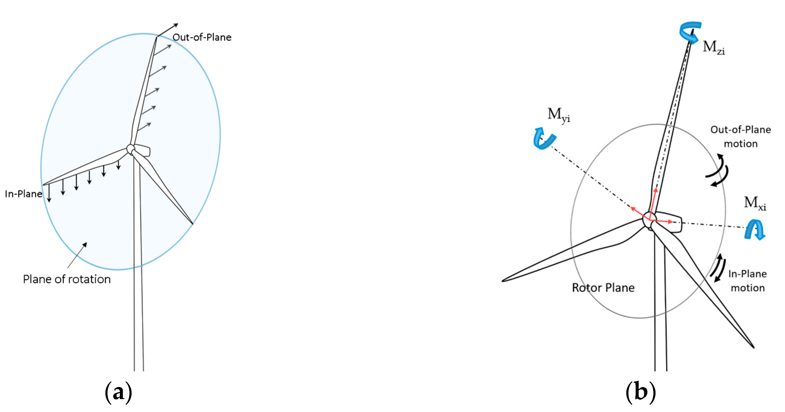
| Mi, Myi | Out-of-plane moment of blade i |
| Mxi | In-plane moment of blade i |
| Mt | Tilt moment (in the nonrotating frame) |
| My | Yaw moment (in the nonrotating frame) |
| Pg,rated | Rated generated power |
| Pg | Generated power |
| S | Solution space |
| Tg | Generator torque |
| Tg,rated | Rated generator torque |
| T(ψ) | MBC transform matrix |
| T−1 | Reverse MBC transform |
| kt | Gain of tilt moment controller |
| ky | Gain of yaw moment controller |
| s | Laplacian variable |
| t | Time |
| βi | Pitch command value of blade i |
| βCPC | Pitch angle provided by the CPC |
| βIPCi | IPC component for pitch signal of blade i |
| βt | Tilt pitch angle (in the nonrotating frame) |
| βy | Yaw pitch angle (in the nonrotating frame) |
| ρ | Decision variable vector |
| ψi | Azimuth angle of blade i |
| ψo | Azimuth offset |
| ψ | Vector with the three azimuth angles |
| ν | Mean wind speed |
| ωg | Rotational generator speed |
| ωg,rated | Rated rotational generator speed |
References
- Njiri, J.G.; Söffker, D. State-of-the-Art in Wind Turbine Control: Trends and Challenges. Renew. Sustain. Energy Rev. 2016, 60, 377–393. [Google Scholar] [CrossRef]
- Lee, J.; Zhao, F. GWEC Global Wind Report; Global Wind Energy Council: Brussels, Belgium, 2022; p. 75. [Google Scholar]
- European Commission. The Commission Calls for a Climate Neutral Europe by 2050; European Commission: Brussels, Belgium, 2018. [Google Scholar]
- Bossanyi, E.A. Individual Blade Pitch Control for Load Reduction. Wind Energy 2003, 6, 119–128. [Google Scholar] [CrossRef]
- Jeong, J.; Park, K.; Jun, S.; Song, K.; Lee, D.-H. Design Optimization of a Wind Turbine Blade to Reduce the Fluctuating Unsteady Aerodynamic Load in Turbulent Wind. J. Mech. Sci. Technol. 2012, 26, 827–838. [Google Scholar] [CrossRef]
- Cheon, J.; Kim, J.; Lee, J.; Lee, K.; Choi, Y. Development of Hardware-in-the-Loop-Simulation Testbed for Pitch Control System Performance Test. Energies 2019, 12, 2031. [Google Scholar] [CrossRef]
- Mulders, S.P.; Pamososuryo, A.K.; Disario, G.E.; van Wingerden, J.-W. Analysis and Optimal Individual Pitch Control Decoupling by Inclusion of an Azimuth Offset in the Multiblade Coordinate Transformation. Wind Energy 2019, 22, 341–359. [Google Scholar] [CrossRef]
- Lu, Q.; Bowyer, R.; Jones, B.L. Analysis and Design of Coleman Transform-Based Individual Pitch Controllers for Wind-Turbine Load Reduction. Wind Energy 2015, 18, 1451–1468. [Google Scholar] [CrossRef]
- Mulders, S.P.; van Wingerden, J.-W. On the Importance of the Azimuth Offset in a Combined 1P and 2P SISO IPC Implementation for Wind Turbine Fatigue Load Reductions. In Proceedings of the IEEE 2019 American Control Conference (ACC), Philadelphia, PA, USA, 10–12 July 2019; pp. 3506–3511. [Google Scholar]
- Spencer, M.D.; Stol, K.A.; Unsworth, C.P.; Cater, J.E.; Norris, S.E. Model Predictive Control of a Wind Turbine Using Short-Term Wind Field Predictions. Wind Energy 2013, 16, 417–434. [Google Scholar] [CrossRef]
- Sierra-García, J.E.; Santos, M. Performance Analysis of a Wind Turbine Pitch Neurocontroller with Unsupervised Learning. Complexity 2020, 2020, 4681767. [Google Scholar] [CrossRef]
- Sierra-Garcia, J.E.; Santos, M. Improving Wind Turbine Pitch Control by Effective Wind Neuro-Estimators. IEEE Access 2021, 9, 10413–10425. [Google Scholar] [CrossRef]
- Mulders, S.; Pamososuryo, A.; van Wingerden, J. Efficient Tuning of Individual Pitch Control: A Bayesian Optimization Machine Learning Approach. J. Phys. Conf. Ser. 2020, 1618, 022039. [Google Scholar] [CrossRef]
- Lara, M.; Garrido, J.; van Wingerden, J.-W.; Mulders, S.P.; Vázquez, F. Optimization with Genetic Algorithms of Individual Pitch Control Design with and without Azimuth Offset for Wind Turbines in the Full Load Region. IFAC-PapersOnLine 2023, 56, 342–347. [Google Scholar] [CrossRef]
- Ragan, P.; Manuel, L. Comparing Estimates of Wind Turbine Fatigue Loads Using Time-Domain and Spectral Methods. Wind Eng. 2007, 31, 83–99. [Google Scholar] [CrossRef]
- Gaertner, E.; Rinker, J.; Sethuraman, L.; Zahle, F.; Anderson, B.; Barter, G.; Abbas, N.; Meng, F.; Bortolotti, P.; Skrzypinski, W.; et al. Definition of the IEA Wind 15-Megawatt Offshore Reference Wind Turbine Technical Report; National Renewable Energy Laboratory: Golden, CO, USA, 2020.
- NREL OpenFAST v3.4.1 Documentation. Available online: https://openfast.readthedocs.io/en/main/ (accessed on 24 April 2023).
- Niranjan, R.; Ramisetti, S.B. Insights from Detailed Numerical Investigation of 15 MW Offshore Semi-Submersible Wind Turbine Using Aero-Hydro-Servo-Elastic Code. Ocean Eng. 2022, 251, 111024. [Google Scholar] [CrossRef]
- Papi, F.; Bianchini, A. Technical Challenges in Floating Offshore Wind Turbine Upscaling: A Critical Analysis Based on the NREL 5 MW and IEA 15 MW Reference Turbines. Renew. Sustain. Energy Rev. 2022, 162, 112489. [Google Scholar] [CrossRef]
- Jonkman, J.; Butterfield, S.; Musial, W.; Scott, G. Definition of a 5-MW Reference Wind Turbine for Offshore System Development; National Renewable Energy Lab., (NREL): Golden, CO, USA, 2009.
- KC, A.; Whale, J.; Evans, S.P.; Clausen, P.D. An Investigation of the Impact of Wind Speed and Turbulence on Small Wind Turbine Operation and Fatigue Loads. Renew. Energy 2020, 146, 87–98. [Google Scholar] [CrossRef]
- Jonkman, B. TurbSim User’s Guide: Version 1.50; National Renewable Energy Lab., (NREL): Golden, CO, USA, 2009.
- IEC 61400-1; Wind Turbines—Part 1: Design Requirements. IEC: Geneva, Switzerland, 2005.
- Novaes Menezes, E.J.; Araújo, A.M.; Bouchonneau da Silva, N.S. A Review on Wind Turbine Control and Its Associated Methods. J. Clean. Prod. 2018, 174, 945–953. [Google Scholar] [CrossRef]
- Abbas, N.J.; Zalkind, D.S.; Pao, L.; Wright, A. A Reference Open-Source Controller for Fixed and Floating Offshore Wind Turbines. Wind Energy Sci. 2022, 7, 53–73. [Google Scholar] [CrossRef]
- Serrano, C.; Sierra-Garcia, J.-E.; Santos, M. Hybrid Optimized Fuzzy Pitch Controller of a Floating Wind Turbine with Fatigue Analysis. J. Mar. Sci. Eng. 2022, 10, 1769. [Google Scholar] [CrossRef]
- NREL MLife|Wind Research|NREL. Available online: https://www.nrel.gov/wind/nwtc/mlife.html (accessed on 25 April 2023).
- Deb, K. An Efficient Constraint Handling Method for Genetic Algorithms. Comput. Methods Appl. Mech. Eng. 2000, 186, 311–338. [Google Scholar] [CrossRef]
- Andrade Aimara, G.A.; Esteban San Román, S.; Santos, M. Control Tuning by Genetic Algorithm of a Low Scale Model Wind Turbine. In Proceedings of the International Workshop on Soft Computing Models in Industrial and Environmental Applications, Salamanca, Spain, 5–7 September 2023; pp. 515–524. [Google Scholar]


| Property | Value |
|---|---|
| Power rating | 15 MW |
| Rotor orientation, configuration | Upwind, 3 blades |
| Cut-in, rated rotor speed | 5 rpm, 7.56 rpm |
| Cut-in, rated, cut-out wind speed | 3 m/s, 10.59 m/s, 25 m/s |
| Drivetrain | Low speed, direct drive |
| Rated generator torque | 19,786,767.5 Nm |
| Electrical generator efficiency | 95.756% |
| Rotor, hub diameter, hub height | 240 m, 7.94 m, 150 m |
| Rotor nacelle assembly mass | 1,070,000 kg |
| Tower mass | 860,000 kg |
| Blade pitch angle limits | 0–90 deg |
| Pitch slew-rate limits | 2 deg/s |
| Generator torque slew-rate limits | 4,500,000 Nm/s |
| Mean Wind Speed (m/s) | Mean OoP Blade Moment (MNm) |
|---|---|
| 14 | 34.94 |
| 16 | 28.68 |
| 18 | 24.03 |
| 20 | 20.33 |
| 22 | 17.23 |
| Control Scheme | Wind Speed (m/s) | |||||
|---|---|---|---|---|---|---|
| 14 | 16 | 18 | 20 | 22 | ||
| CPC | (M) (MNm) | 24.07 | 23.08 | 25.06 | 30.8 | 25.39 |
| CPC + IPC_P2 | (M) (MNm) | 16.91 | 14.97 | 17.26 | 22.06 | 13.84 |
| kt (deg/(MNm)) | 18.94·10−2 | 19.22·10−2 | 23.72·10−2 | 8.4·10−2 | 14.21·10−2 | |
| ky (deg/(MNm)) | 31.61·10−2 | 17.12·10−2 | 11.53·10−2 | 4.2·10−2 | 25.36·10−2 | |
| ψo (deg) | 0 | 0 | 0 | 0 | 0 | |
| CPC + IPC_P2ψ | (M) (MNm) | 16.9 | 14.9 | 17.23 | 20.87 | 13.84 |
| kt (deg/(MNm)) | 17.35·10−2 | 17.13·10−2 | 23.65·10−2 | 9.6·10−2 | 14.66·10−2 | |
| ky (deg/(MNm)) | 29.07·10−2 | 21.97·10−2 | 11.54·10−2 | 11.2·10−2 | 25.69·10−2 | |
| ψo (deg) | 0.55 | 0.17 | 5.66 | 19.36 | 0.01 | |
| CPC + IPC_I1 | (M) (MNm) | 17.00 | 16.27 | 18.74 | 22.32 | 16.73 |
| kt (deg/(MNms)) | 2.98·10−2 | 2.5·10−2 | 0.93·10−2 | 0.77·10−2 | 0.49·10−2 | |
| ky (deg/(MNms)) | 2.98·10−2 | 2.5·10−2 | 0.93·10−2 | 0.77·10−2 | 0.49·10−2 | |
| ψo (deg) | 0 | 0 | 0 | 0 | 0 | |
| CPC + IPC_I1ψ | (M) (MNm) | 14.32 | 14.67 | 16.33 | 17.22 | 13.45 |
| kt (deg/(MNms)) | 5.74·10−2 | 9.19·10−2 | 13.82·10−2 | 9.07·10−2 | 11.63·10−2 | |
| ky (deg/(MNms)) | 5.74·10−2 | 9.19·10−2 | 13.82·10−2 | 9.07·10−2 | 11.63·10−2 | |
| ψo (deg) | 85.86 | 74.8 | 61.05 | 79.89 | 76.52 | |
| CPC + IPC_I2 | (M) (MNm) | 16.8 | 16.25 | 18.23 | 20.07 | 15.96 |
| kt (deg/(MNms)) | 3.39·10−2 | 2.21·10−2 | 1.93·10−2 | 2.79·10−2 | 0.068·10−2 | |
| ky (deg/(MNms)) | 1.82·10−2 | 1.08·10−2 | 0.21·10−2 | 0.14·10−2 | 1.86·10−2 | |
| ψo (deg) | 0 | 0 | 0 | 0 | 0 | |
| CPC + IPC_I2ψ | (M) (MNm) | 14.32 | 14.61 | 16.12 | 17.22 | 13.45 |
| kt (deg/(MNms)) | 5.73·10−2 | 19.4·10−2 | 11.65·10−2 | 8.93·10−2 | 12.28·10−2 | |
| ky (deg/(MNms)) | 5.76·10−2 | 12.9·10−2 | 20.14·10−2 | 9.55·10−2 | 11.01·10−2 | |
| ψo (deg) | 88.75 | 75.33 | 62.27 | 77.50 | 76.85 | |
| Control Scheme | (M) (MNm) | (β) (%) | STD(Pg) (MW) | STD(ωg) (rpm) | ||||||||
|---|---|---|---|---|---|---|---|---|---|---|---|---|
| Case 1 | Case 2 | Case 3 | Case 1 | Case 2 | Case 3 | Case 1 | Case 2 | Case 3 | Case 1 | Case 2 | Case 3 | |
| CPC | 23.67 | 25.62 | 29.68 | 4.91 | 4.38 | 4.07 | 0.46 | 0.60 | 0.80 | 0.23 | 0.30 | 0.40 |
| CPC + IPC_P2 | 17.55 | 18.79 | 20.45 | 48.9 | 52.5 | 50.61 | 0.46 | 0.61 | 0.81 | 0.23 | 0.31 | 0.41 |
| CPC + IPC_P2ψ | 17.50 | 18.71 | 19.72 | 50 | 52.3 | 51.57 | 0.46 | 0.61 | 0.81 | 0.23 | 0.31 | 0.41 |
| CPC + IPC_I1 | 18.80 | 21.94 | 21.68 | 41.6 | 44.6 | 46.45 | 0.46 | 0.61 | 0.80 | 0.23 | 0.31 | 0.40 |
| CPC + IPC_I1ψ | 16.60 | 17.25 | 17.51 | 38.8 | 43.4 | 49.45 | 0.46 | 0.60 | 0.81 | 0.23 | 0.30 | 0.41 |
| CPC + IPC_I2 | 18.77 | 20.3 | 21.63 | 41.0 | 42.2 | 46.64 | 0.46 | 0.60 | 0.80 | 0.23 | 0.30 | 0.41 |
| CPC + IPC_I2ψ | 16.66 | 17.18 | 17.47 | 39.6 | 43.8 | 49.47 | 0.46 | 0.61 | 0.81 | 0.23 | 0.30 | 0.41 |
| Control Scheme | (MNm) | STD(Mt) (MNm) | (MNm) | STD(My) (MNm) | ||||||||
|---|---|---|---|---|---|---|---|---|---|---|---|---|
| Case 1 | Case 2 | Case 3 | Case 1 | Case 2 | Case 3 | Case 1 | Case 2 | Case 3 | Case 1 | Case 2 | Case 3 | |
| CPC | 6.678 | 7.516 | 9.282 | 3.84 | 3.89 | 4.17 | 2.582 | 3.298 | 3.568 | 3.50 | 4.02 | 4.17 |
| CPC + IPC_P2 | −0.208 | −0.252 | 0.118 | 2.86 | 3.15 | 3.62 | −0.294 | −0.067 | −0.207 | 2.73 | 3.22 | 3.55 |
| CPC + IPC_P2ψ | −0.209 | −0.27 | 0.158 | 2.86 | 3.15 | 3.61 | −0.219 | 0.588 | 1.202 | 2.70 | 3.19 | 3.42 |
| CPC + IPC_I1 | −0.015 | −0.038 | 0.024 | 3.37 | 4.53 | 4.36 | 0.039 | −0.072 | 0.100 | 3.46 | 4.61 | 3.97 |
| CPC + IPC_I1ψ | −0.004 | −0.008 | −0.006 | 2.56 | 2.76 | 3.25 | −0.011 | −0.002 | −0.013 | 2.24 | 2.45 | 2.89 |
| CPC + IPC_I2 | −0.06 | −0.032 | 0.018 | 3.30 | 3.52 | 3.83 | −0.015 | 0.247 | 0.188 | 3.91 | 4.84 | 4.43 |
| CPC + IPC_I2ψ | −0.002 | −0.004 | −0.003 | 2.64 | 2.86 | 3.24 | −0.008 | −0.007 | −0.011 | 2.33 | 2.59 | 2.87 |
Disclaimer/Publisher’s Note: The statements, opinions and data contained in all publications are solely those of the individual author(s) and contributor(s) and not of MDPI and/or the editor(s). MDPI and/or the editor(s) disclaim responsibility for any injury to people or property resulting from any ideas, methods, instructions or products referred to in the content. |
© 2023 by the authors. Licensee MDPI, Basel, Switzerland. This article is an open access article distributed under the terms and conditions of the Creative Commons Attribution (CC BY) license (https://creativecommons.org/licenses/by/4.0/).
Share and Cite
Lara, M.; Mulders, S.P.; van Wingerden, J.-W.; Vázquez, F.; Garrido, J. Analysis of Adaptive Individual Pitch Control Schemes for Blade Fatigue Load Reduction on a 15 MW Wind Turbine. Appl. Sci. 2024, 14, 183. https://doi.org/10.3390/app14010183
Lara M, Mulders SP, van Wingerden J-W, Vázquez F, Garrido J. Analysis of Adaptive Individual Pitch Control Schemes for Blade Fatigue Load Reduction on a 15 MW Wind Turbine. Applied Sciences. 2024; 14(1):183. https://doi.org/10.3390/app14010183
Chicago/Turabian StyleLara, Manuel, Sebastiaan Paul Mulders, Jan-Willem van Wingerden, Francisco Vázquez, and Juan Garrido. 2024. "Analysis of Adaptive Individual Pitch Control Schemes for Blade Fatigue Load Reduction on a 15 MW Wind Turbine" Applied Sciences 14, no. 1: 183. https://doi.org/10.3390/app14010183
APA StyleLara, M., Mulders, S. P., van Wingerden, J.-W., Vázquez, F., & Garrido, J. (2024). Analysis of Adaptive Individual Pitch Control Schemes for Blade Fatigue Load Reduction on a 15 MW Wind Turbine. Applied Sciences, 14(1), 183. https://doi.org/10.3390/app14010183