Fault Diagnosis Strategy Based on BOA-ResNet18 Method for Motor Bearing Signals with Simulated Hydrogen Refueling Station Operating Noise

Featured Application

In this paper, the vibration data of CWRU motor bearings is used as the original data to simulate the real working conditions of motor bearings in the working environment of hydrogen station by simulating the noise signal of hydrogen station. Then, the BOA-ResNet18 model is used to diagnose the faults of the added noise signals, and the accuracy of the fault diagnosis is very high, and the experimental results show that this model can be applied in the fault diagnosis of hydrogen station equipment under the working conditions of hydrogen station.

Abstract

The harsh working environment of hydrogen refueling stations often causes equipment failure and is vulnerable to mechanical noise during monitoring. This limits the accuracy of equipment monitoring, ultimately decreasing efficiency. To address this issue, this paper presents a motor bearing vibration signal diagnosis method that employs a Bayesian optimization (BOA) residual neural network (ResNet). The industrial noise signal of the hydrogenation station is simulated and then combined with the motor bearing signal. The resulting one-dimensional bearing signal is processed and transformed into a two-dimensional signal using Fast Fourier Transform (FFT). Afterwards, the signal is segmented using the sliding window translation method to enhance the data volume. After comparing signal feature extraction and classification results from various convolutional neural network models, ResNet18 yields the best classification accuracy, achieving a training accuracy of 89.50% with the shortest computation time. Afterwards, the hyperparameters of ResNet18 such as InitialLearnRate, Momentum, and L2Regularization Parameter are optimized using the Bayesian optimization algorithm. The experiment findings demonstrate a diagnostic accuracy of 99.31% for the original signal model, while the accuracy for the bearing signal, with simulated industrial noise from the hydrogenation station, can reach over 92%.

1. Introduction

Hydrogen is a zero-emission, efficient, and versatile energy carrier that can be produced from a variety of sources. It is a crucial solution to replace unsustainable fossil fuels and reduce carbon emissions in the 21st century [1]. Notably, the hydrogen refueling station plays a vital role in the hydrogen energy industry chain, serving as a critical infrastructure that connects hydrogen suppliers with fuel vehicle users downstream [2]. A compressor, hydrogen dispenser, and hydrogen storage vessel are critical pieces of equipment in a hydrogen refueling station. Among these, the rolling bearing is an essential component in the oil pump motor of the compressor. The bearings are exposed to forces in all directions due to the complex working environment. Without proper coordination with other parts or maintenance, they are prone to damage. The failure of a rolling bearing can result in extensive economic losses and may even compromise worker safety, leading to a breakdown in the entire industrial production process. For this reason, the diagnosis of faults in rolling bearings holds immense practical significance.

With the development of artificial intelligence algorithms, deep learning algorithms can realize the extraction of equipment fault characteristics from monitoring data and diagnose their deep faults, and they have been widely used in the field of machinery fault diagnosis. Therefore, in the bearing fault diagnosis, many scholars at home and abroad propose a variety of deep learning algorithms to identify and classify the bearing faults. Feng et al. [3] proposed a multi-level denoising technique based on Improved Singular Value Decomposition (ISVD) and Intrinsic Time Scale Decomposition (ITD) combined with an improved deep residual network (ResNet) for rolling bearing fault diagnosis. The experimental results show that the proposed method can realize more accurate fault diagnosis of rolling bearings in high noise environment compared with other methods. Guoqian Jiang et al. [4] proposed a new interpretable deep learning model called Multi Wavelet Kernel Convolutional Neural Network (MWKCNN) for fault diagnosis. Diwang Ruan et al. [5] detailed the physical characteristics of bearing acceleration signals to guide the design of CNN. The results show that physically guided convolutional neural network (PGCNN) with rectangular input shape and rectangular convolutional kernel works better than baseline convolutional neural network with higher accuracy and less uncertainty. Manu Krishnan et al. [6] proposed a new method for modeling dynamic systems by combining wavelets with input-output dynamic modal decomposition (ioDMD). The experimental results show that the algorithm still performs well under the influence of noise. Xiaoyu et al. [7] proposed a Residual Network (ResNet)-based deep migration diagnostic model for bearing failures by combining Wavelet Packet Transform (WPT) and Multicore Maximum Mean Difference (MK-MMD). And the comparative experiments under different working loads and speeds were carried out on two test benches. The results show that the proposed method has good fault diagnosis and noise prevention ability and is suitable for the task of working condition transition. Xudong Li et al. [8] optimize and improve the Neural Architecture Search (NAS) according to the field of automated machine learning, and apply it to the field of fault diagnosis. Tian Zhang et al. [9] proposed a slope and threshold with tanh function adaptive activation function (STAC-tanh), which improves the problem of the activation function compressing part of the fault information in the traditional neural network. A convolutional neural network is a typical deep learning method that has been widely used for image recognition. Chunran Huo et al. [10] proposed an improved adaptive dimension transformed convolutional neural network (ADC-CNN) to improve the accuracy by 9% for the problem for which 1D-CNN could not fully utilize the feature extraction. Among the classical models of convolutional neural networks include LeNet, AlexNet, GoogleNet, VGG, ResNet, DRSN, and so on.

In the field of bearing fault diagnosis, the current motor bearing fault data collected by Western Reserve University is more widely used and widely used as the base database for neural network training models [11,12,13].

Lin Pei et al. [14] proposed a bearing fault diagnosis method based on a one-dimensional convolutional generative adversarial network (1D-DCGAN) and one-dimensional convolutional self encoder (1D-CAE), which realized high-precision diagnosis across different devices with small samples. Shanshan Ding et al. [15] proposed a rolling bearing fault diagnosis method based on reparametrized VGG (RepVGG), and the recognition and classification accuracy of vibration signals reaches more than 95%. Hao Wei [16] and Xu Min et al. [17] used the CWRU bearing database as the basic data and used wavelet packet transform and other data processing methods to introduce the processed signals into the improved ResNet model. The signal after processing is imported into the modified ResNet model by using wavelet packet transform and other data processing methods for computational analysis, which effectively solves the overfitting problem and achieves good results at the same time. In addition, Lanjun Wan et al. [18] proposed a convolutional adaptive model integrating a feature extraction module, a domain adaptive module, and a fault identification module, and used ResNet network as a feature extractor, which can extract the required features from the original signal. In addition, Deep Residual Neural Network (DRSN) is a network architecture proposed in 2020 based on ResNet plus a soft threshold function. Li Shichao et al. [19] used the DRSN network architecture to achieve intelligent identification and filtering of inertial force interference signals and instrumentation noise signals to improve the accuracy of aerodynamic testing. Hao Yin et al. [20] proposed a new fault diagnosis method for pressure relief valves, combining the elastic weight consolidation (EWC) algorithm with the Deep Residual Shrinkage Network (DRSN), and the experimental validation of the model yielded an average accuracy rate of 98.8%, with an average loss of 0.095.

In summary, the accuracy of fault identification in the literature regarding convolutional neural networks in the field of fault diagnosis is summarized as

Table 1. Comparison of fault diagnosis accuracy of different models.

Literature	Diagnostic Methods	Accuracy
Literature [4]	MResNet-SVM	97.40%
Literature [15]	MWKCNN	98.36%
Literature [19]	FB-LSTM	98.60%
Literature [17]	RepVGG	98.02%
Literature [21]	GMA-DRSN	91.2%

.

Jun Gu et al. [21] proposed a rolling bearing fault diagnosis method based on variational modal decomposition (VMD), continuous wavelet transform (CWT), convolutional neural network (CNN), and support vector machine (SVM), and verified the effectiveness of the proposed method using the bearing vibration data and spindle unit failure test bench data from Case Western Reserve University (CWRU), and the average classification accuracy of the former was 99.9% and the average classification accuracy of the latter was 90.15%. Wang Huan et al. [22] proposed a novel attention-guided joint learning convolutional neural network (JL-CNN) for mechanical equipment condition monitoring. The fault diagnosis task (FD task) and signal denoising task (SD task) are integrated into an end-to-end CNN architecture, and good noise robustness is achieved through dual-task joint learning. In addition, CNNs are widely used in fault diagnosis of various mechanical devices [23,24]. Jia Linsan, Wang Hui, and Zongmeng et al. [25,26,27] extracted data from vibration signals generated when various machines such as bearings are damaged, and detected and processed the signals of various faults by using end-to-end CNN model based on GNR (GTFE-Net), MS-CNN, and other methods, and the final results showed that the optimized convolutional neural network model can be widely used in the field of fault diagnosis of mechanical equipment.

In the computational process of neural networks, the choice of hyperparameter values such as learning rate, batch size, hidden layer size, etc. will directly affect the performance and training speed of neural networks. Bayesian optimization is a method to find the optimal hyperparameter settings by modeling the relationship between known hyperparameter configurations and model performance. It uses Bayesian inference and real-time feedback mechanisms to gradually improve the selection of hyperparameters, thus improving the performance of the model. Chang Miao et al. [28] proposed a wind turbine bearing fault diagnosis strategy based on Bayesian optimization and improved convolutional neural network (CNN) for the problems of weak rolling bearing fault features, difficult extraction and low diagnostic efficiency of wind turbine. The results show that the accuracy of the optimized fault diagnosis model rises by 12.85% compared with the original model. Tang Liang et al. [29] designed a Bayesian optimization improved LeNet-5 algorithm and carried out experiments through the bearing database, which showed that the bearing fault diagnosis model constructed by this algorithm had an accuracy of 99.94% in the training set, 99.89% in the validation set, and the accuracy of the test set also reached 99.65%. S. Jayalakshmy et al. [30] used Bayesian optimization of hyperparameters such as the initial learning rate, the strength of the L2 regularization, and the stochastic gradient descent momentum in a GoogleNet network to improve the computational accuracy of the original GoogleNet network by 7.35%. Shengnan Tang et al. [31] optimized a CNN neural network using Bayesian optimization algorithm and compared the computational results with LeNet5, which was 2.92% more accurate than LeNet5. Chen et al. [32] proposed a fault pulse extraction and feature enhancement method for bearing fault diagnosis. The method is able to extract weak fault pulses from bearing signals containing strong background noise, periodic harmonics and strong random pulses. The anti-interference ability of the model is improved. Wang Yuxuan et al. [33] proposed a new method for fault diagnosis of motor bearings based on Extreme Gradient Growth Tree (XGboost) and Bayesian optimization to achieve more accurate identification of vibration signals in the system.

In the operational setting of hydrogen refueling stations, bearings frequently become contaminated with acoustic noise, including mechanical vibration. Therefore, it is necessary to employ denoising techniques to mitigate the impact of noise on the acquired signals [34]. When comparing current denoising techniques, it is evident that wavelet denoising and wavelet packet thresholding represent optimal methods for removing mid- and high-frequency noise from large samples with varying degrees of denoising. This conclusion was reached after comparing various denoising techniques, including empirical modal decomposition and variational modal decomposition [34,35,36,37,38]. Hai Qiu et al. [39] compared the performance of wavelet-decomposition-based denoising methods and wavelet-filtering-based denoising methods based on mechanical defect signals. The comparison results show that wavelet filtering is more suitable and reliable for detecting the weak features of mechanical impulse-like defect signals, while wavelet decomposition denoising method is more effective in smoothing signal detection. Diletta Sacerdoti et al. [40] compared signal analysis techniques for rolling bearing diagnosis and proposed a diagnostic method based on the combination of cepstrum prewhitening and squared-envelope spectroscopy, which was combined with experimental analysis. Finally, it was suggested that the best way to perform condition monitoring should be a combination of classical signal-based and new data-driven techniques. Babu T et al. [41] used Debauchies Wavelet-02 (DB-02) to diagnose faults in journal bearings and classified the faults using artificial neural networks (ANN). The classification result was 85.7%. In addition, the advantages of using DB-02 wavelet technique over conventional wavelet technique in high-speed machines were experimentally analyzed.

The Fourier transform is a method of transforming a signal from a time-domain signal to a frequency-domain signal, and the Fast Fourier Transform (FFT) is an algorithm for efficiently computing the discrete Fourier transform. FFT processing of signals can achieve higher signal accuracy. Zuolu Wang [42] developed a wireless three-axis rotor sensing system (ORS) and used FFT and Hilbert envelope analysis to greatly improve the accuracy of their system troubleshooting. Şahin Yavuz [43], experimentally and by using the FFT method, investigated the effect of deceleration time on the root mean square (RMS) value of residual vibration (RV). The effect of the result’s agreement shows that the FFT method is very effective for studying transient vibration problems in complex systems.

Dongwen Li et al. [44] proposed a combined model based on RSM-XGBoost and KF algorithm to study the remaining life prediction problem of an aircraft engine, and solved the noise influence problem by adding a Carr filter to achieve higher life prediction accuracy. Cong Wang et al. [45] worked on analyzing the elite RSH by estimating the desired approximation error. Based on the distribution of non-zero elements in the Markov chain transfer matrix, the search process of the elite RSH was classified into three categories, and a general framework for estimating the approximation error, called error analysis, was proposed.

To process the CWRU bearing database used in this study, vibration signal window shifting and wavelet denoising were applied. The signals underwent diagnosis and classification using ResNet18. Some hyperparameters were optimized with the Bayesian optimization algorithm to improve fault diagnosis accuracy. Finally, noise was added to replicate real hydrogenation station conditions, ensuring model anti-interference capabilities against noise signals.

This paper analyzes and processes the bearing failure signals of Western Reserve University (CWRU). The bearing vibration signal is transformed from a one-dimensional signal to a two-dimensional signal using the Fast Fourier Transform (FFT). The signal samples are split to expand the number of samples by using the vibration signal window panning. Due to the presence of various noise sources, such as mechanical noise and electromagnetic interference, the vibration signal may be affected during the motor bearing signal acquisition process. Therefore, it is necessary to denoise the decomposed bearing signal. In this paper, we denoise the CWRU signal using a 5-level Symlet-5 wavelet and suppress or eliminate the noise signal using a soft threshold function. The signal is then inputted into various convolutional neural network models for computation. After analyzing the computing time and computational accuracy, this paper selects the resnet18 network to construct the training model. Next, the parameters of the trained neural network model are tuned using Bayesian optimization, based on the theory of neural network hyperparameter optimization, to achieve better fault diagnosis results. To simulate the hydrogen refueling station’s production environment and verify the model’s anti-interference ability, noise signals of 70 dB, 80 dB, 90 dB, and random pulse signals were added to the CWRU bearing signal. The final test results demonstrate that the BOA-ResNet18 model maintains high fault diagnosis accuracy even with the added noise signals, indicating excellent anti-interference ability.

2. Vibration Signal Data Processing and Feature Enhancement

The computational accuracy of convolutional neural networks is highly related to the diversity of data samples and the obviousness of the samples’ features. Too few data samples and inconspicuous data features can lead to overfitting in the calculation process, resulting in inaccurate calculation results. In order to solve the above problems, image data enhancement and data expansion techniques are introduced. In image processing, common data enhancement operations include rotation, flipping, panning, scaling, cropping, and so on.

2.1. Signal Analysis

Western Reserve University (CWRU) bearing data acquisition tests were measured under different horsepower motor fan end and drive end bearing vibration data, of which the drive end bearing was for 6205-2RS JEM SKF (produced by SKF, Gothenburg, Sweden) deep groove ball bearings, the fan end bearing was for 6203-2RS JEM SKF deep groove ball bearings, and for which the SKF6025 bearings sampling frequency was 12 kHz and 48 kHz and the SKF6023 sampling frequency was 12 kHz. SKF6023 sampling frequency was 12 kHz. The experiment used EDM treatment to form a single point of failure on the inner and outer rings and balls of the bearings, and the bearings with different failure parts were operated at different speeds and frequencies. Finally, the vibration values of the inner ring, outer ring, rolling element, and normal state of the bearing were recorded, respectively.

In this paper, the vibration signal data of the drive end bearing at a frequency of 12 kHz and a rotational speed of 1772 r/min are selected, and the specific data are shown in

Table 2. Sample set of CWRU bearing failure data.

Bearing Type	Motor Load (Horsepower)	Motor SPEED (r/min)	Fault Diameter (mm)	Fault Location	Sample Set (Number of Data Points Per Sample/Number of Samples)
Drive end bearing (6205-2RS JEM SKF)	1	1772	0.1778	Inner ring	122,100/1
				Rolling element	122,100/1
				Outer ring	122,100/3
			0.3556	Inner ring	122,100/1
				Rolling element	122,100/1
				Outer ring	122,100/1
			0.5334	Inner ring	122,100/1
				Rolling element	122,100/1
				Outer ring	122,100/3
			0.7112	Inner ring	122,100/1
				Rolling element	122,100/1
				Outer ring	0

.

2.2. Data Expansion

As can be seen from Table 1, the samples of each type of bearing faults are too small, so it is necessary to introduce data expansion processing techniques to split the data. Since the dataset is one-dimensional, this paper utilizes the Fast Fourier Transform (FFT) to convert the data into two-dimensional frequency domain signals and then uses sliding window panning to divide the signals. The total number of samples is maximized and the computational effect of the neural network is enhanced while preserving the temporal vibration signal coherence as well as the signal characteristics.

The Fourier Transform transforms a function from the time domain to the frequency domain. The Discrete Fourier Transform (DFT) is an application of the Fourier Transform to discretize the Fourier Transform. It can decompose a signal into a series of sine and cosine sums for spectrum analysis, filtering, signal processing, etc., while the Fast Fourier Transform (FFT) is an efficient way of solving the Discrete Fourier Transform. The DFT formula is as follows:

$$X\left(k\right)=\sum [x\left(n\right)\times e^{(\frac{-j\times 2\pi kn}{N})}]$$

(1)

where N denotes the number of sampling points, x(n) denotes the input signal, and k represents the frequency domain index. The FFT splits the DFT computation into several small-scale DFT computations and then recombines them and obtains the overall result by butterfly operation. The formula is as follows:

$$X\left(k\right)=E\left(k\right)+W_k^N\times 0[k]$$

(2)

$$X\left(k+\frac{N}{2}\right)=E\left(k\right)-W_k^N\times 0[k]$$

(3)

E[k] is the input elements at even index positions, 0[k] is the input elements at odd index positions. $W_k^N$is the rotation factor, and N is the total number of input elements.

The rotation factor $W_k^N$ is

$$W_k^N=e^{\frac{2\pi ikn}{N}}$$

(4)

where n is the subscript of the sequence, k is the subscript of the frequency, and N is the sequence size. In arithmetic code, the rotation factors are usually stored in complex form, and the size of the rotation factors is automatically adjusted by calling the data.

The FFT algorithm computes the DFT of these components recursively by decomposing the signal into parity components and then combining the results to obtain the final spectrum. Using the FFT to convert one-dimensional values into Fourier-transformed frequency domain values can provide higher accuracy for periodic signals or signals that contain multiple frequency components. It can provide more accurate frequency components and amplitude values, since noise signals have a certain anti-interference ability. Taking the 0.1778 mm fault diameter inner ring fault point as an example, the time–frequency domain graph obtained after the transformation is as Figure 1.

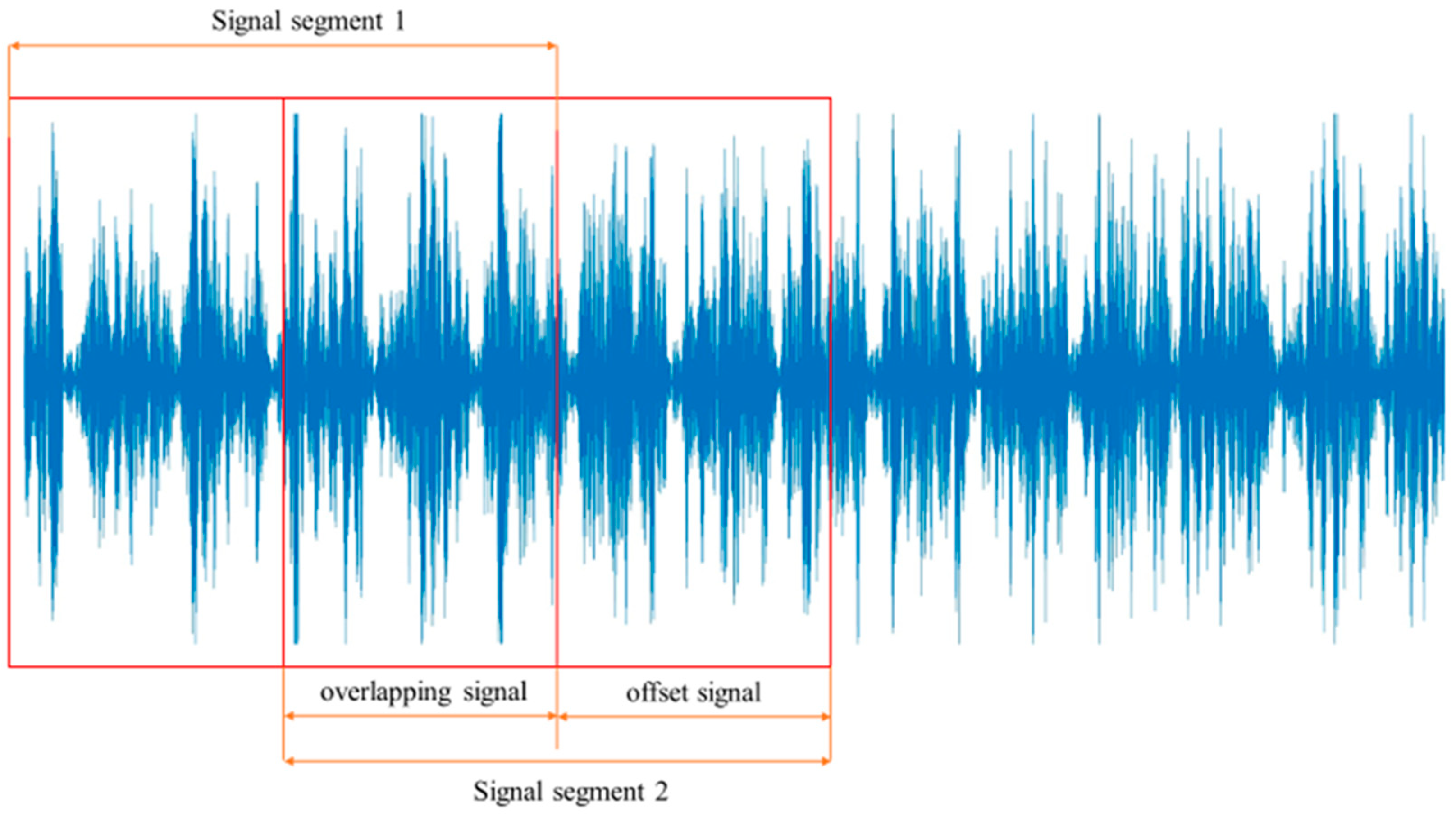
Since the signal is a long sequence signal and the data samples are too small, the signal must be processed by window function segmentation after the FFT transform. These windows usually have overlapping parts. Due to the boundary effect of the window function, this processing method will lead to the appearance of spectral leakage and sub-flap, which will affect the accuracy of the analysis results. To solve this problem, in this paper, the signal segmentation is performed by sliding window panning. By panning between each window, the overlap between windows can be reduced, thus minimizing the effects of spectral leakage and sub-flap, as shown in Figure 2. Assuming that the length of the original signal is N, the length of the window is M, and the step length (overlap rate) of the panning is L, after the panning, then, the length H of the signal obtained by window panning can be calculated as follows:

When the overlap is less than the window length:

$$H=L+(K-1)\times L$$

(5)

When the overlap is greater than the window length:

H = M + (K − 1) × L

(6)

K is the smallest integer that makes the right end of the equation greater than or equal to N.

In order to ensure the coherence of the time series vibration signals and maximize the number of samples, the signal overlap rate is set to be 512, and the window step size is 1024. Each signal is classified into 200 sample sets; the training and 12 kHz and 1772 r/min drive end bearing failure signal are divided according to the ratio of 30%. As shown in Figure 3, The specific description of the sample set is shown in

Table 3. CWRU sample set segmentation.

Sample Label	Fault Diameter (mm)	Fault Location	Training Set/Test Set
1	—	trouble-free	140/60
2	0.1778	inner ring	140/60
3		rolling element	140/60
4		outer ring	140/60
5	0.3556	inner ring	140/60
6		rolling element	140/60
7		outer ring	140/60
8	0.5334	inner ring	140/60
9		rolling element	140/60
10		outer ring	140/60
11	0.7112	inner ring	140/60
12		rolling element	140/60

.

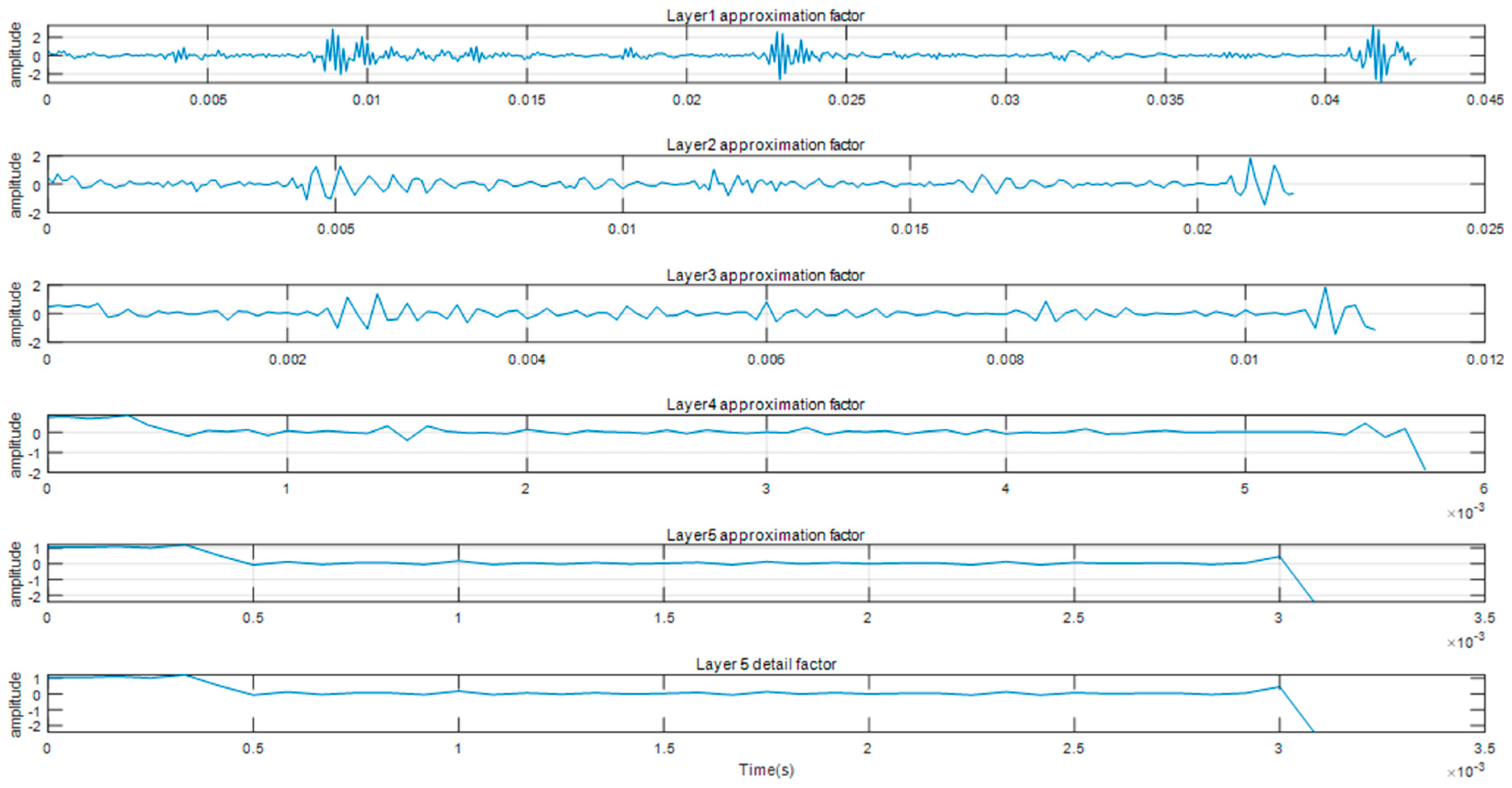
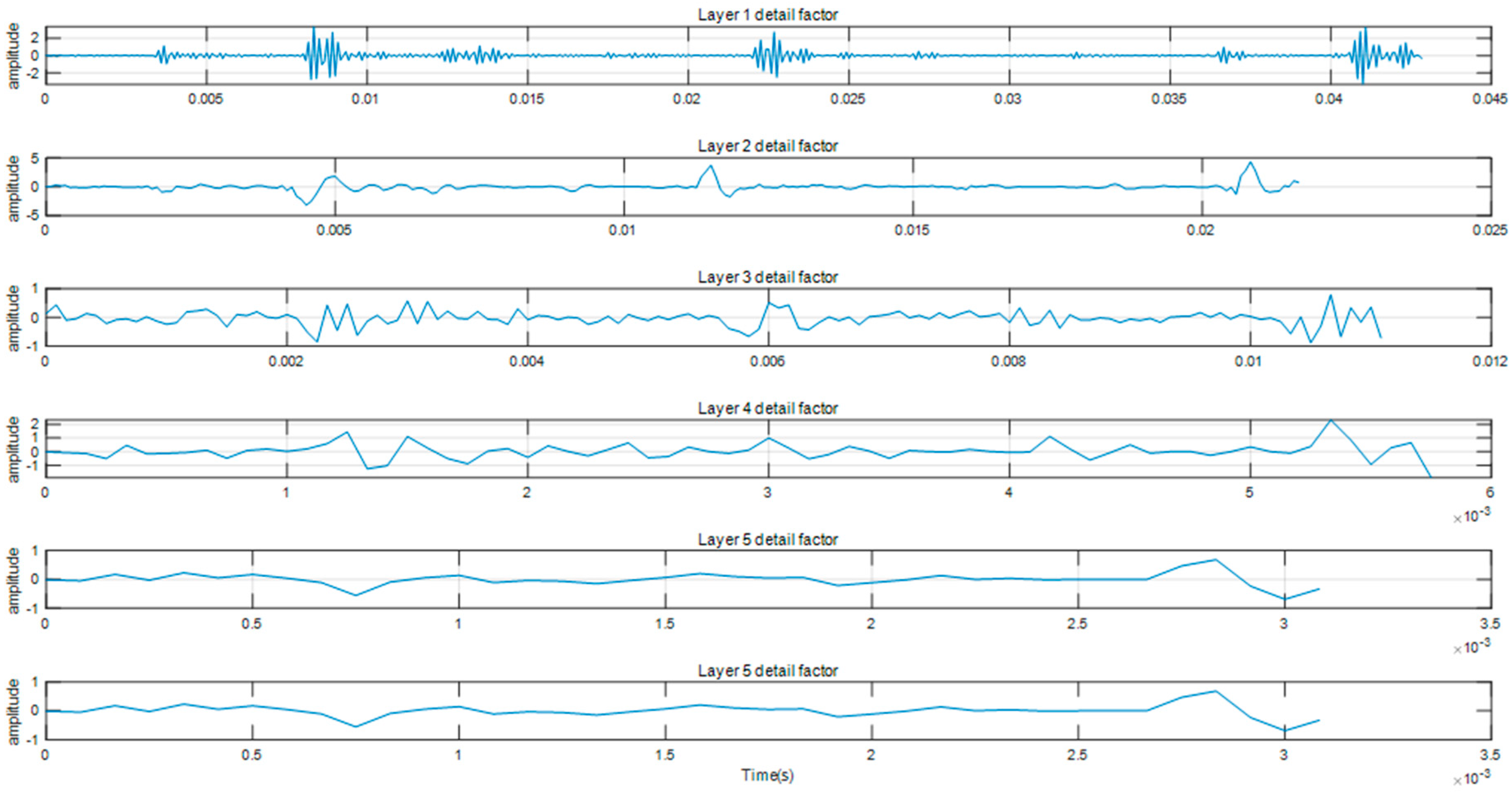
2.3. Wavelet Decomposition Denoising

In the CWRU bearing test operation environment, the motor bearing vibration signal is affected by a variety of noise sources, including mechanical noise, electromagnetic interference, environmental vibration, and so on. These noise signals will be mixed with the signals generated by the bearing to form the final vibration signal. Therefore, the presence of noise signals needs to be taken into account when analyzing and processing the CWRU-bearing dataset. In this paper, wavelet denoising is used to suppress the noise interference to extract the bearing fault characteristics and perform accurate fault diagnosis.

Wavelet thresholding denoising is a method of signal denoising using the results of the wavelet transform, which is a technique that converts a signal into the wavelet domain by applying wavelet decomposition. It utilizes the wavelet transform to extract the frequency domain information of the signal and suppresses or eliminates the noise components of the signal by thresholding the wavelet coefficients.

$$F(jw)={\int }_{-\infty }^{+\infty }f\left(t\right)e^{-j\omega t}dt={\int }_{-\infty }^{+\infty }f\left(t\right)[\mathit{cos}\left(wt\right)-jsin(wt\left)\right]dt$$

(7)

Equation (6) is the Fourier transform, and the wavelet transform is in principle changing the basis function in the Fourier transform to a wavelet. The wavelet transform formula is as follows:

$$F(a,\tau )=\frac{1}{\sqrt{a}}{\int }_{-\infty }^{+\infty }f\left(t\right)\times \psi (\frac{t-\tau }{a})dt$$

(8)

τ is the time shift, a is the scaling factor, and Ψ(t) is the wavelet basis function.

The following are the steps to perform wavelet denoising:

(1) Perform wavelet decomposition: First, select a suitable wavelet basis function according to the application requirements and signal characteristics. Common wavelet basis functions include Daubechies, Haar, symlets, etc. Second, the signal to be denoised is represented as a discrete sequence, x(n), n = 0, 1,..., N − 1. Then, at each scale, the selected wavelet basis function is used to perform a convolution operation with the signal to obtain the Approximation Coefficients and Detail Coefficients.

In a continuous situation:

$$c_j\left(k\right)=\sum _n{h}_{\phi }(n-2k)c_{j+1}(n)$$

(9)

$$d_j\left(k\right)=\sum _n{h}_{\psi }(n-2k)c_{j+1}(n)$$

(10)

c_j(k) denotes the kth coefficient in the jth level of approximation coefficients, d_j(k) denotes the kth coefficient in the jth level of detail coefficients, and c_(j+1)(n) denotes the nth coefficient in the jth + 1st level of approximation coefficients, and furthermore, the h_φ and h_ψ in the equation represent the low-pass and high-pass filter coefficients of the wavelet function (Mother Wavelet), respectively, which determine the characteristics of wavelet decomposition.

Typically, the approximation coefficients represent the low frequency components of the signal at that scale, while the detail coefficients represent the high frequency components of the signal at that scale. This is shown in Figure 4 and Figure 5.

(2) Calculate the threshold of the wavelet coefficients: select an appropriate threshold selection method, such as hard threshold or soft threshold. Calculate the threshold of each wavelet coefficient according to the selected thresholding method. The formula for hard thresholding is as follows:

$$w_{thr}=\left\{\begin{array}{c}w \left|w\right|\ge thr\\ 0 \left|w\right|\le thr\end{array}\right.$$

(11)

The soft threshold formula is as follows:

$$w_{thr}=\left\{\begin{array}{cc}\left[sgn\left(w\right)\right](\left|w\right|-thr)& \left|w\right|\ge thr\\ 0& \left|w\right|\le thr\end{array}\right.$$

(12)

where thr is the given threshold and w is the wavelet coefficient.

Comparing the hard threshold and soft threshold denoising methods, the points |w| ≤ thr are directly set to zero in the hard threshold, which makes it easy to cause the discontinuity of the wavelet coefficients, while the soft threshold denoising method eliminates this discontinuity and ensures the smoothness of the reconstructed signal. Therefore, the soft threshold denoising method is chosen in this paper.

(3) Reconstructing the signal: using the threshold wavelet coefficients, the inverse wavelet transform is performed to reconstruct the signal after noise reduction.

In this paper, the Symlet-5 wavelet is used to perform 5-level wavelet noise reduction processing on the CWRU signal, and the noise signal is suppressed or eliminated by the soft threshold function. The signal after the noise reduction process is as Figure 6.

In Figure 6, the orange signal is the denoised signal and the blue signal is the original signal. The signal can be seen after soft threshold filtering removes most of the noise components in the signal while preserving the vibration frequency of the signal as well as the amplitude and other important features. In addition, wavelet threshold denoising smooths the signal, making the fluctuations of the signal smoother, resulting in the denoised signal compared to the original signal in some moments of the vibration amplitude being smaller, but on the whole, it can still reflect the vibration trend and changes to facilitate the identification of subsequent features.

The denoised 12 kHz, 1772 r/min drive end bearing fault signals are similarly categorized and numbered and divided into denoised sample sets. The sample set is described in

Table 4. CWRU denoising sample set partitioning.

Sample Label	Fault Diameter (mm)	Fault Location	Training Set/Test Set
101	—	trouble-free	140/60
102	0.1778	inner ring	140/60
103		rolling element	140/60
104		outer ring	140/60
105	0.3556	inner ring	140/60
106		rolling element	140/60
107		outer ring	140/60
108	0.5334	inner ring	140/60
109		rolling element	140/60
110		outer ring	140/60
111	0.7112	inner ring	140/60
112		rolling element	140/60

.

3. Neural Network Selection and Computation

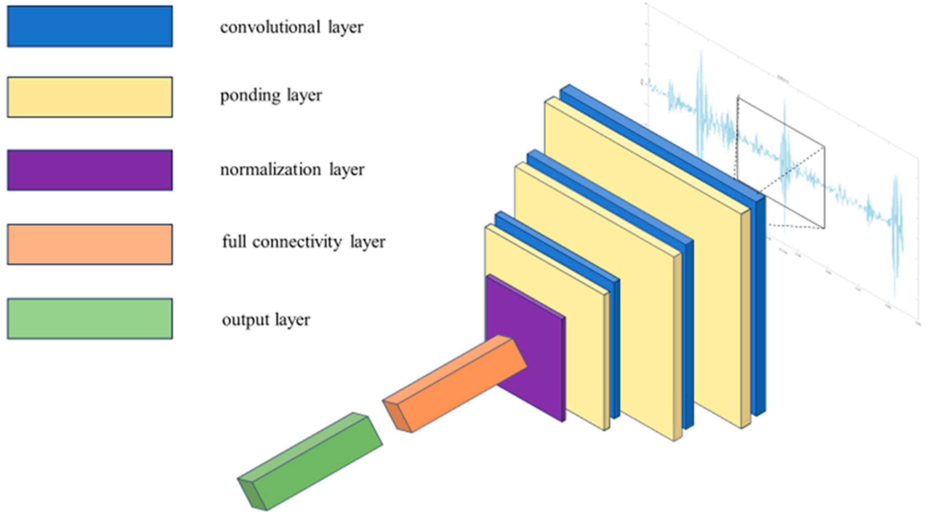
A convolutional neural network (CNN) is a deep learning model specialized in processing data with a grid structure (e.g., images and speech, etc.). It extracts features from the input data through convolutional and pooling operations and performs tasks such as classification or regression through fully connected layers.

As shown in Figure 7, the basic structure of the convolutional neural network mainly consists of an input layer, a convolutional layer, a pooling layer, a normalization layer, a fully connected layer, and an output layer. Among them, the convolutional layer performs the convolution operation by capturing the local structure and texture information of the input data and generating the feature map. Activation function nonlinearization is required after convolution to introduce the nonlinear nature of the model. Common activation functions include ReLU, Sigmoid, and tanh. The pooling layer is used to reduce the spatial size of the feature map and the number of parameters. The normalization layer is responsible for normalizing the input data to make the data distribution more stable. The fully connected layer is usually located at the end of the convolutional neural network and its role is to map the high-level features to the corresponding classes or targets. The output layer can vary depending on the needs of the task. For classification tasks, a softmax layer is usually used to transform the output of the model into a vector representing the probability of each category.

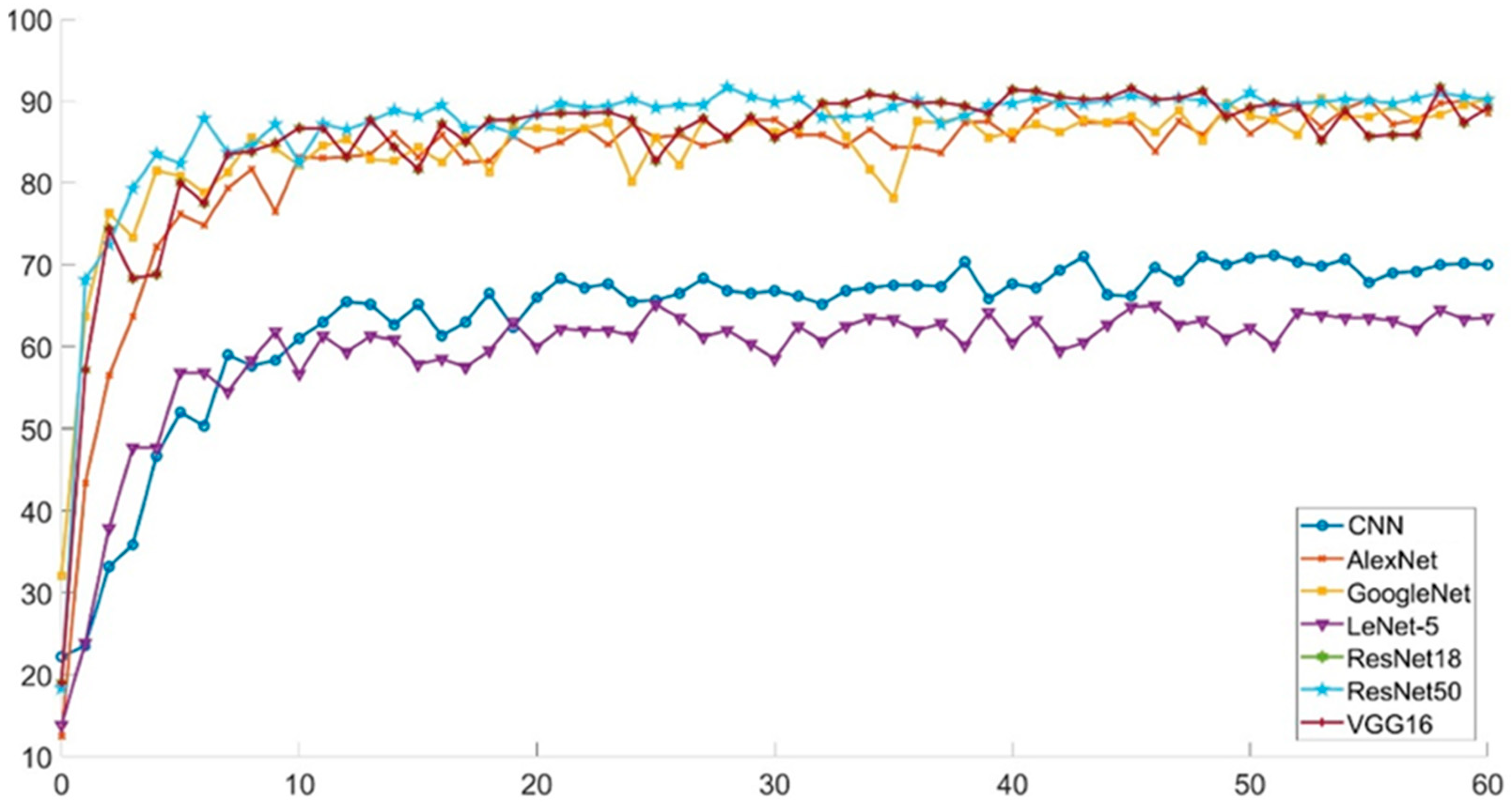
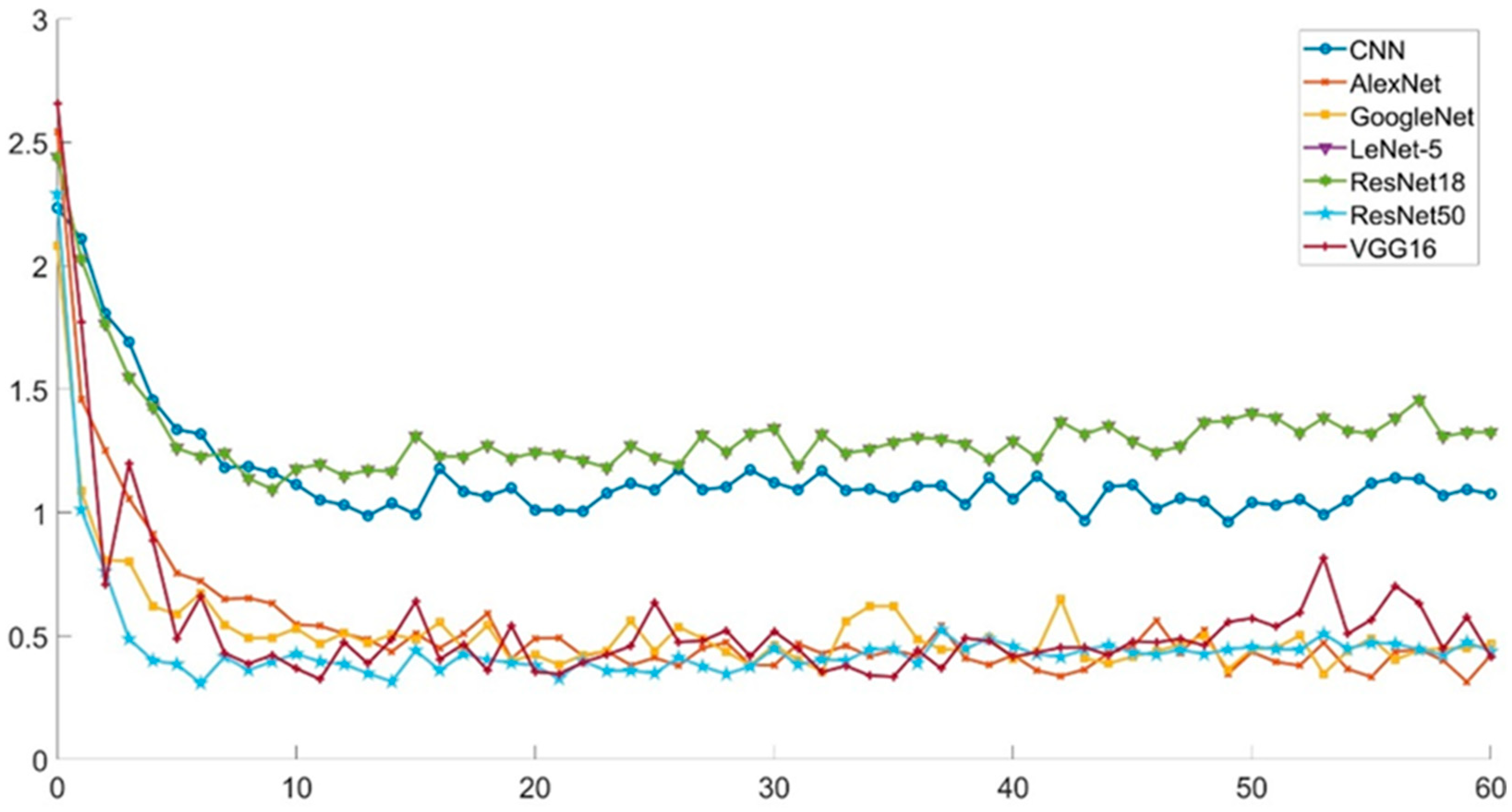
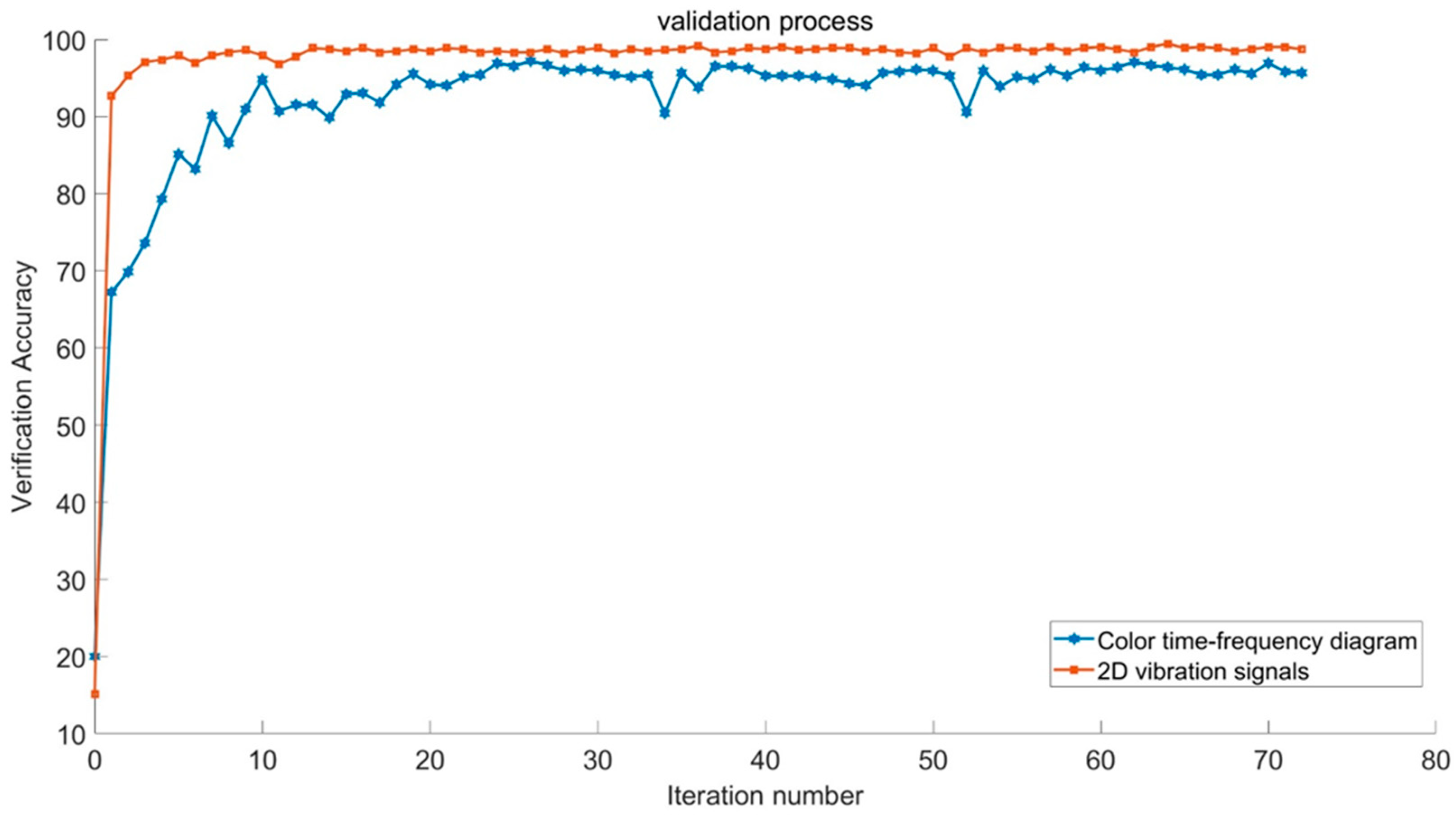
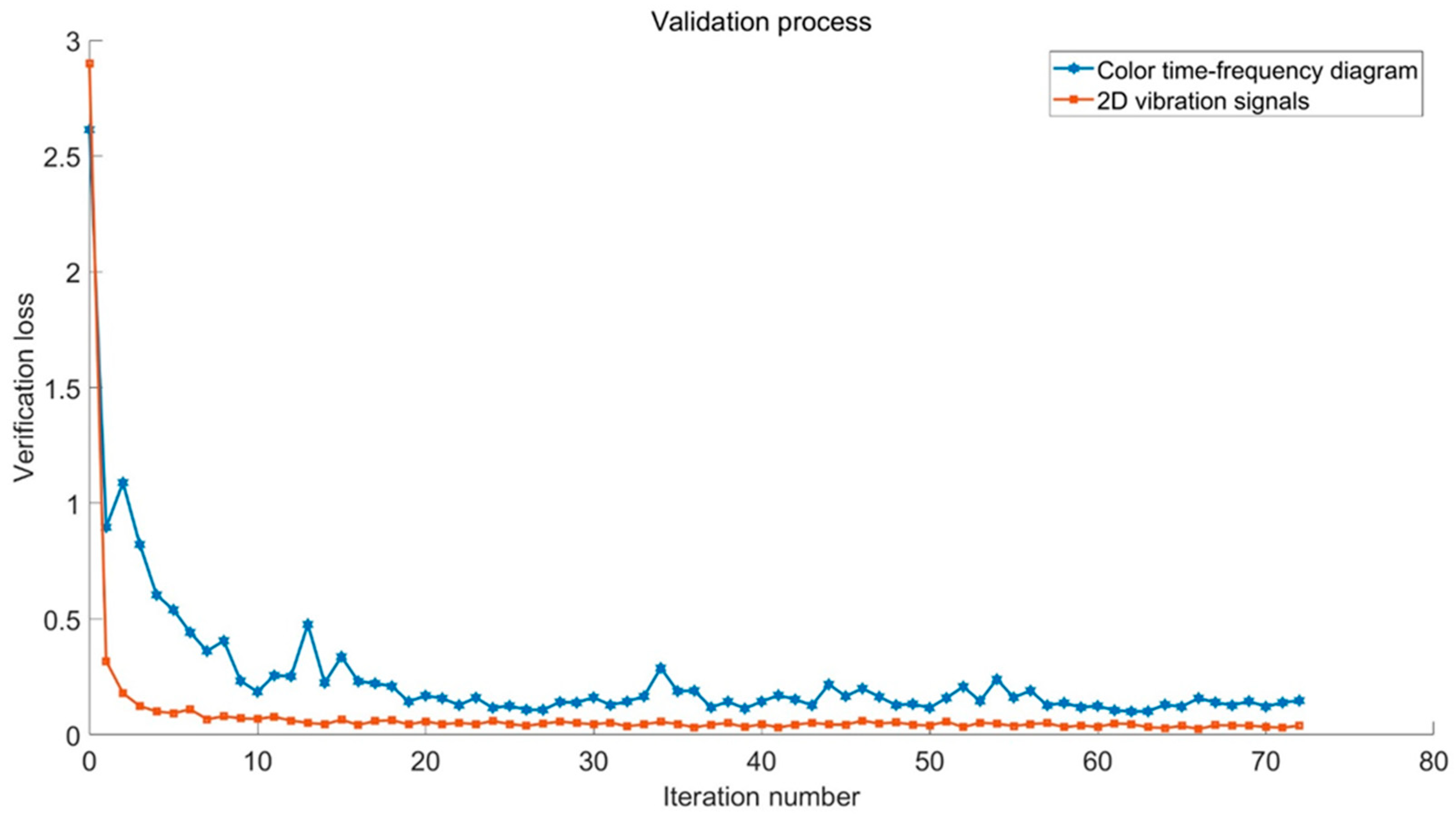
Different convolutional neural network models can be obtained by combining and connecting multiple layer structures of a convolutional neural network in different ways. The common convolutional neural network models are LeNet-5, AlexNet, VGGNet, GoogleNet, ResNet, and so on. The sample set in Table 2 and Table 3 is imported into the convolutional neural network model, and the accuracy and loss comparison graphs obtained are as Figure 8 and Figure 9:

In the working environment of hydrogenation station, the oil pump motor speed is usually in the range of 1000 r/min to 3000 r/min, and the drive end working frequency is usually low compared with the test simulation frequency, and in the occasional failure, will reach 10 kHz and above. Therefore, in order to fit the actual production environment, this paper selects the vibration signal data of the drive end bearing at 12 kHz frequency and 1772 r/min speed. The results of the training accuracy of the denoised samples are summarized in

Table 5. Comparison of training results of different network models.

Network Structure	Accuracy (Denoised Samples)	Training Time(s)
Single CNN	73.67%	311
AlexNet	87.83%	346
GoogleNet	89.83%	637
LeNet-5	67.33%	401
ResNet18	89.50%	251
ResNet50	90.17%	1065
VGG16	87.33%	1009

.

Comparing the training accuracy and training time of each model, the training effect of ResNet18 network is the best. Therefore, ResNet18 network is chosen to build the training model in this paper.

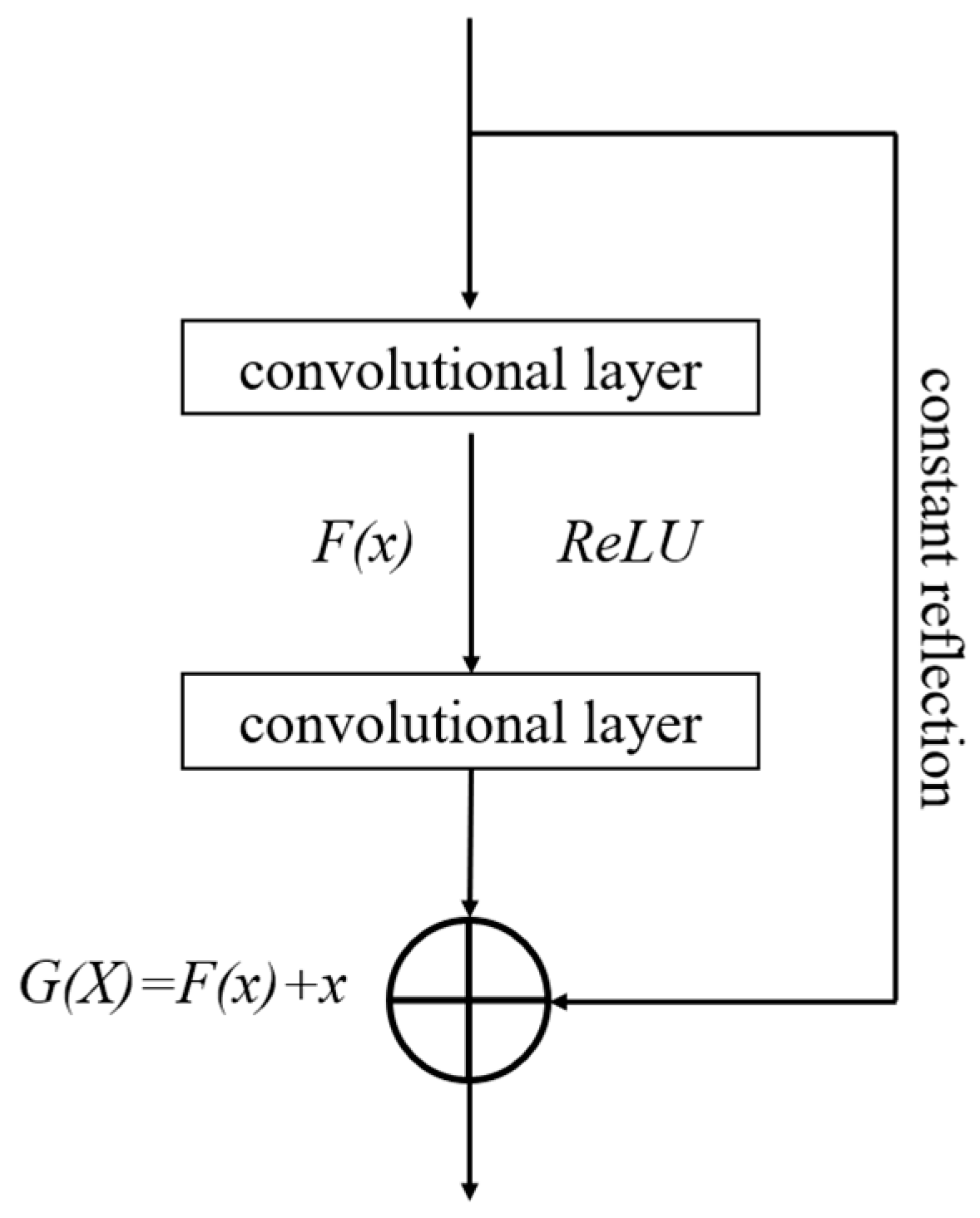
3.1. ResNet18

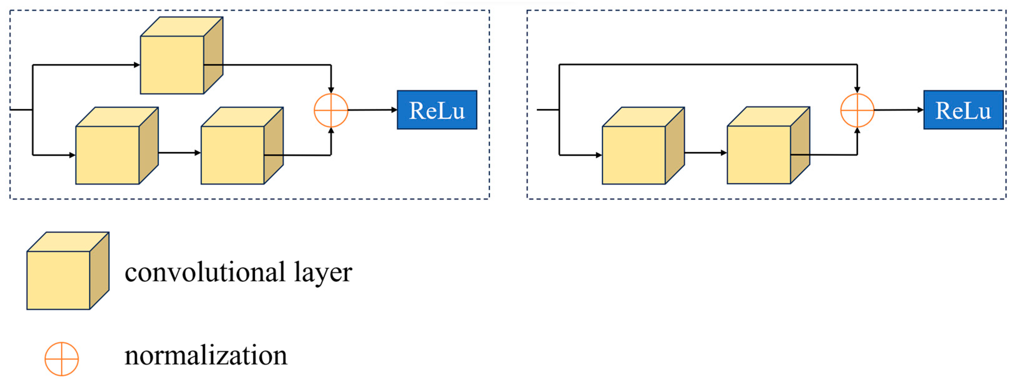
Residual neural network is a new deep convolutional neural network architecture proposed by Kaiming He et al. in 2015, and its main core idea is to solve the gradient vanishing and expression bottleneck problem in deep neural networks by introducing “residual blocks”. Traditional deep networks have the problem of gradient vanishing, as the number of network layers increases, the backpropagated gradient signal becomes weaker and weaker, resulting in training difficulties. Residual blocks, on the other hand, allow direct connections across layers, making it easier to transfer information. The residual block structure is shown in Figure 10.

In Figure 10, x is the input, F(x) is the mapping function, and G(x) = F(x) + x is the constant mapping function. By constant mapping, it means that G(x) = x when F(x) tends to 0. The corresponding mathematical expression for the residual block is:

$$\begin{gathered} y_l=h\left(x_l\right)+F(x_l,W_l) \\ {x}_{l+1}=f\left(y_l\right) \end{gathered}$$

(13)

where x_l and x_(l+1) represent the input and output of the lth residual unit, respectively, F() represents the residual function, h(x_l) = x_l denotes the constant mapping, and f is the ReLU activation function. Based on Equation (12), the learning feature from shallow l to deep L can be obtained as:

$$x_L=x_l+\sum _{i=l}^{L-1}F(x_l,W_l)$$

(14)

The introduction of residual blocks into the residual connection structure can play key roles, such as connecting and transferring gradients, learning residuals, extracting high-level features, and increasing network depth. These roles make the residual connection structure have better convergence, stronger expressiveness, and higher performance in training deep neural networks.

By combining different numbers of residual blocks, residual neural network architectures with different numbers of layers can be derived. Some of the more common ones are ResNet-18, ResNet-34, ResNet-50, ResNet-101, and ResNet-152. The numerical designation of these ResNet models indicates the number of layers. For example, ResNet-18 consists of 18 convolutional layers, while ResNet-50 consists of 50 convolutional layers. As the number of layers increases, the network becomes deeper and is able to learn more complex feature representations.

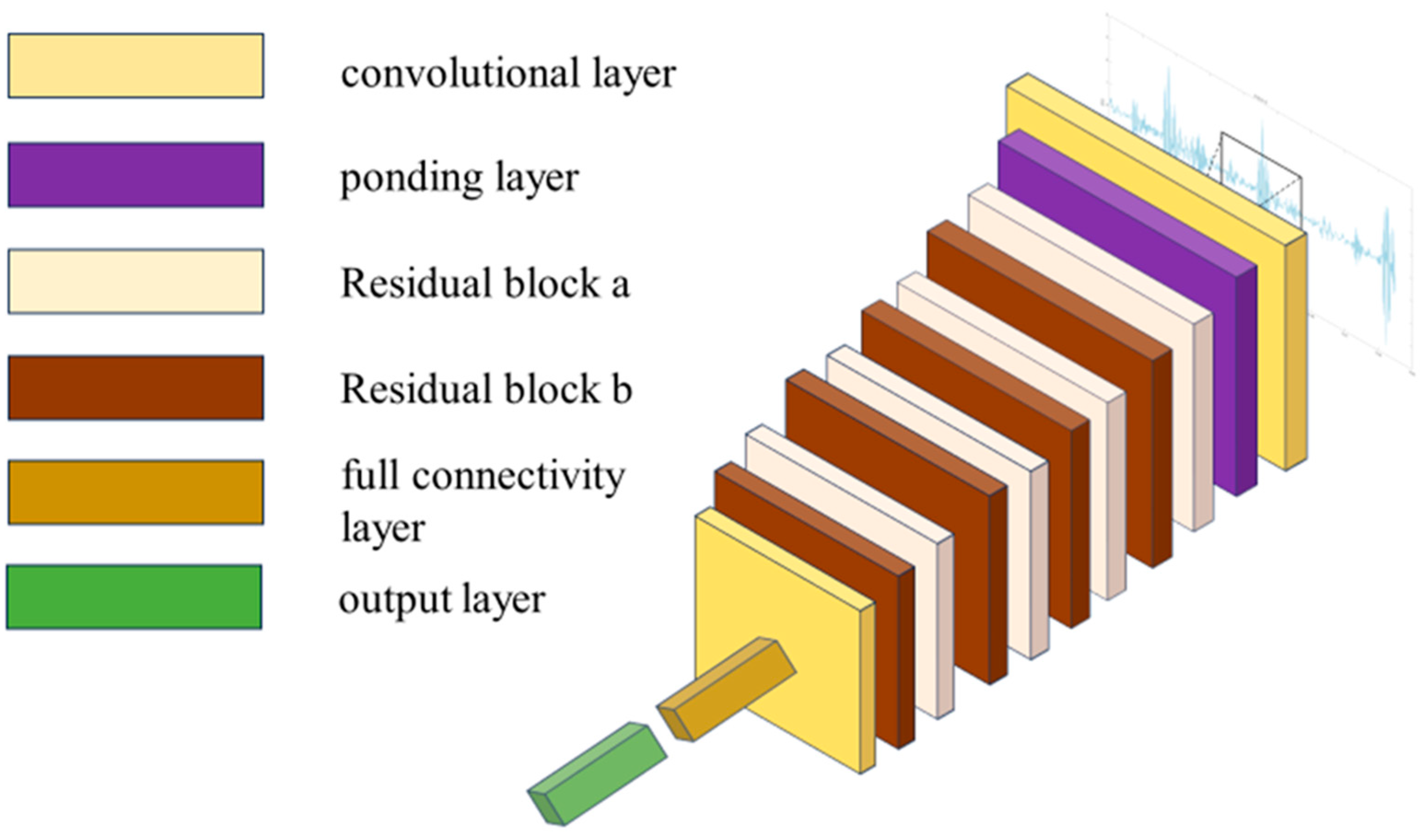
As can be seen from Section 3.1, ResNet-18 is chosen for fault classification recognition in this paper, which consists of four residual modules, each containing two convolutional layers and a jump connection. These convolutional layers typically have a 3 × 3 convolutional kernel size and use the ReLU activation function. Between each residual module, downsampling operations are used to reduce the size of the feature maps. The ResNet-18 structure is shown in Figure 11 and Figure 12.

The network input is an RGB image with a size of 224 × 224 pixels and three channels. The output corresponds to ten different failure modes. To extract features and generate 64 output channels, the input image undergoes a convolution operation using 64 convolution kernels, each with a size of 3 × 3, a stride of 2, and a padding of 1. The convolutional layer’s output size is 112 × 112 × 64 in the ResNet-18 network. The network has four residual connected structures. The convolution operation’s step size is 2 in residual blocks a-1 and b-1, reducing the output feature maps’ spatial size by half while keeping the number of channels the same. This is to preserve more spatial information in the deeper features. In residual blocks a-2 and b-2, the convolution operation has a step size of 2 and the number of channels is doubled. This results in the output feature map being reduced by half in size. The purpose of this is to increase the number of channels in deeper features and further decrease the size of the feature map. Residual blocks a-3 and b-3 use a step size of 2 for the convolution operation, which doubles the number of channels and reduces the spatial size of the output feature map by half. This helps to extract deeper features and increase the number of channels. In residual blocks a-4 and b-4, the number of channels is doubled while the spatial size of the output feature map is reduced by half, but the step size of the convolution operation is 1. The network’s expressive power was improved by increasing the number of channels in deeper features. The ResNet-18 network feature-extracted and downsampled the image to produce an n × 10 × 14 × 14 feature map (n is the MiniBatchSize value). This was followed by an average pooling layer of size 14 × 14 and a Softmax classifier to produce an n × 10 × 1 × 1 feature image. The specific parameters of the network structure are shown in

Table 6. Network architecture parameters.

Layer Type	Output Size
input layer	224 × 224 × 3
convolutional layer 1	112 × 112 × 64
residual block a-1	112 × 112 × 64
residual block b-1	112 × 112 × 64
residual block a-2	56 × 56 × 128
residual block b-2	56 × 56 × 128
residual block a-3	28 × 28 × 256
residual block b-3	28 × 28 × 256
residual block a-4	14 × 14 × 512
residual block b-4	14 × 14 × 512
Average pooling layer	14 × 14 × 512
full connectivity layer	1 × 1 × 10

.

4. Bayesian Optimization of ResNet18

4.1. Over-Parameter Range Setting

Convolutional neural networks require some parameters to be set before training, which are not learned by the optimization algorithm and must be set manually by humans. Such manually set parameters are called hyperparameters. The setting of hyperparameters directly affects the performance of the model and the training process to a large extent. The following are some common hyperparameters in convolutional neural network training:

• InitialLearnRate refers to the extent to which the model parameters are updated during each iteration. Choosing an appropriate learning rate ensures that the objective function converges to a local extreme at the appropriate time. To avoid falling into the local optimum in the early stages, a larger learning rate is usually set initially to reduce the network’s attenuation. There are different types of decay, such as exponential decay:

  $$Ir=Ir0\times d_r^{t/d_s}$$

  (15)

  The Ir0 is the initial learning rate, d_r is the decay factor, t is the number of iterations, and ds is the number of decay steps.
• L2Regularization Parameter: L2 regularization is used to control the complexity of the model and prevent overfitting. The L2Regularization parameter determines the weight of the regularization term in the overall loss function. Its paradigm loss function L(W) is calculated as follows:

  $$L(W)={\sum }_{i=1}^n{(y_i-f(x_1\left)\right)}^2$$

  (16)

  The λ is the hyperparameter controlling the size of the regularization term and ωi is the size of the coefficient corresponding to the ith model vector.
• Momentum: In neural network learning, stochastic gradient descent (SGD) is a common optimization algorithm. However, it is very easy to fall into the problem of local minima during the operation; in addition, SGD also has the problem of slow convergence speed. To improve the shortcomings of SGD algorithm, Momentum algorithm is introduced. Momentum is a technique used to speed up the convergence of optimization algorithms. It reduces oscillations during parameter updates and allows the optimization algorithm to converge to the optimal solution faster by introducing a momentum term that takes into account the direction of the previous gradient update. The basic momentum formula is as follows:

  $$\begin{gathered} v_t=\gamma v_{t-1}+\eta {\nabla }_{\theta }J\left(\theta \right) \\ \theta =\theta -v_t \end{gathered}$$

  (17)

  v_t is the momentum term, which represents the cumulative information of the gradient; γ is the momentum factor; it controls how much the previous gradient affects the current update; η is the learning rate, which specifies the step size of each update; and ∇_θJ(θ) is the current gradient.

4.2. Optimization Test Analysis

The most popular hyperparametric optimization algorithms are stochastic search, grid search, and Bayesian optimization. Bayesian optimization methods tend to perform better in parametric optimization problems. Compared to grid search and random search, Bayesian optimization methods are usually able to find better parameter combinations with the same computational resources. Li Dongwen et al. [39] used the random search algorithm to optimize an aircraft engine vibration signal prediction model, and the difference between the test error and the training error was calculated to be more than 1 in the experimental process, which did not meet the accuracy requirements of this experiment, and Cong Wang et al. [40] optimized the calculation of the random algorithm to meet the computational requirements. The global search algorithm takes too long and costs too much to be applied in this experiment.

Bayesian optimization is an optimization method used to find the global optimum of a black box function (optimal objective function). Among them, the prior function and the collection function are the core processes of the Bayesian optimization algorithm. The prior function mainly utilizes Gaussian process regression:

f(x) ~ GP(m(x), k(x, x’))

(18)

GP denotes a Gaussian process, m(x) is the mean function, and k(x, x’) is the covariance (or kernel) function. A Gaussian process is a probabilistic model that characterizes the distribution of a function by a mean vector and a covariance matrix based on a collection of points in the input space. Bayesian optimization tuning using the Gaussian process can take into account the previous parameter information to continuously update the prior function and guide the next optimal choice, which greatly saves computation time.

The collection function is an important part of the Bayesian optimization process used to select the next combination of hyperparameters to evaluate. The construction of the collection function based on the mean and variance calculated by the Gaussian process reflects the degree to which the numerical points are worth searching. And the extreme point of this function is the next search point. Choosing the appropriate collection function can help the algorithm converge to the optimal solution quickly and accurately. Common sampling functions include Thompson Sampling, Expected Improvement, and Upper Confidence Bound. The collection process is represented by Equations (18) and (19):

$$x_{i+1}=\underset{x\in X}{\max }\lambda (x,D_{1:i})$$

(19)

$$r_i=\left|y^{*}-y_i\right|$$

(20)

r is the total loss, X is the decision space, λ(x,D_1:i) is the collection function, and y* is the optimal solution.

To summarize, the Delikere process sampling is chosen in this paper. Assume that the Dirichlet sampling of this model is G1, where the underlying distribution of G1 is H1 and the concentration parameter is α. Then, the result of the sampling can be expressed as follows for any segmentation point t:

$$G1(t)=\sum _{i=1}^{\infty }wi\times \delta (\theta i)$$

(21)

where wi is a random variable satisfying the Dirichlet distribution, i.e., wi ~ Dir(α), and θi is a random variable sampled from the underlying distribution H1.

The Bayesian optimization process is as follows:

• Select initial parameters and evaluate for the objective function.
• Construct the agent model of the Bayesian optimization algorithm, i.e., the prior function and the learning function.
• Select the next parameter point xi to be evaluated.
• Execute the objective function on the selected parameter point and record the results.
• Add the new parameter objective function evaluation data to the existing data set and retrain the agent model.
• Determine whether the stopping condition is satisfied; if not, return to step (3) until the optimal value parameter point is output.

Bayesian optimization was used to optimize some hyperparameters of ResNet18, the number of iteration rounds was set to 30, the maximum number of iterations per round was set to 120, the sampling function was chosen to sample the Delicacy process, and the range of hyperparameter settings is shown in

Table 7. Hyperparameter optimization and range.

Hyperparameterization	Minimum	Maximum
InitialLearnRate	0.001	0.1
L2Regularization Parameter	1 × 10−10	1 × 10−2
Momentum	0.8	0.98
Optimizers	RMSprop, Adam, Sgdm

.

Based on the above selected range of hyper-parameters, the BOA-ResNet18 network was used for experimental validation. Setting the range of hyperparameter optimization based on previous expert experience [31,32], and the results showed that the Bayesian optimized.

Network achieved 99.31% computational accuracy. Comparison of the fault diagnosis accuracy with other literature for raw CWRU signals is shown in

Table 8. Comparison of diagnostic results.

Literature	Diagnostic Methods	Accuracy
This paper	BOA-RseNet18	99.31%
Literature [17]	FB-LSTM	98.60%
Literature [21]	RepVGG	98.02%
Literature [42]	GMA-DRSN	91.2%

.

It can be seen that the neural network model built in this paper has the best fault diagnosis accuracy for the original signal of CWRU bearings.

The accuracy as well as the validation loss are shown in Figure 13 and Figure 14.

Figure 13 shows the classification of the model on the test set, and it can be seen that the model has a very low false positive rate, which means that it is able to make judgments on different fault types very well. Therefore, the model performs well in achieving fault-type judgment.

In Figure 15, the green squares indicate samples that are categorized accurately, i.e., the model correctly predicts the samples into that category, while the red squares indicate samples that are categorized incorrectly, i.e., the model incorrectly predicts the samples into other categories. It can be seen that the model predicts well. To explore the accuracy of the BOA-ResNet18 network for the calculation results of signals in other formats, and to avoid the possibility of the algorithm calculating a single sample, the denoised two-dimensional vibration signals were converted to three-channel color time–frequency plots by time–frequency analysis, as shown in Figure 16. In the color time-frequency diagram clearly depicts the relationship between the signal frequency over time and also expresses the corresponding amplitude magnitude by the change of different colors.

The above processed signals are classified and numbered, and imported into the BOA-ResNet18 network for calculation, and the results show that the fault diagnosis accuracy of the color time–frequency diagram signals reaches 95.42%. This result proves that the BOA-ResNet18 network can achieve better accuracy and loss value with fewer iterations and a shorter running time under different fault data types, and the optimization of the network can be accomplished by continuously adjusting the parameters. The validation set obtained is shown in Figure 17 and Figure 18.

4.3. Validation of Model Immunity to Interference

In the production environment of a hydrogen refueling station, the bearings experience varying loads while the signal acquisition process is affected by on-site mechanical noise contamination. Therefore, to simulate real working conditions and verify the BOA-ResNet18 network’s generalization ability for various signals, this study introduces Gaussian noise to the original vibration signals to model mechanical noise in the hydrogenation plant.

$$SNR=10\times lg\frac{Ps}{Pn}$$

(22)

The average signal power (Ps) and average noise power (Pn) are used to calculate the signal-to-noise ratio (SNR) on a logarithmic scale expressed in decibels (dB), whereby dB = 10 × lgSNR. To simulate actual working conditions, this study adds three different values of SNR (70 dB, 80 dB, and 90 dB) since the bearing vibration signal typically has an SNR between 70 dB and 90 dB. The added noise signal is shown in Figure 19.

Additionally, the harsh operating conditions of hydrogen refueling stations and the continuous operation of compressors cause bearings to typically experience fatigue rupture, scoring, or wear caused by foreign object intrusion. As a result, this proposes adding random pulse signals to simulate the sudden changes in vibration signal waveforms that result from faults. The resulting simulated fault signal can be expressed as follows:

$$y\left(t\right)=x\left(t\right)+noise\left(t\right)+f\left(t\right)$$

(23)

where x(t) represents the original bearing signal and noise(t) represents the Gaussian noise signal:

$$noise\left(t\right)=A\times e^{{(-((t-t_0)}^2 / (2\times {sigma}^2)\left)\right)}$$

(24)

where f is the frequency of the signal, A is the amplitude of the noise signal, t₀ is the center time of the noise signal, and sigma is the standard deviation of the noise signal. f(t) is a random pulse signal:

$$f\left(t\right)=A\times P\left(t-t_0\right)\times rand$$

(25)

where A represents the pulse’s amplitude, P(t − t₀) represents the pulse function, t₀ represents the pulse’s start time, and rand represents a random number.

Existing experiments indicate that the amplitude range of random pulse signals of industrial motor bearings is typically about seven times greater than that of signals in the normal state [35,36]. To account for the frequency of oil pump motor bearing faults, each signal fragment contains five additional sampling points for random pulse signal collection.

As shown in Figure 20, an increase in decibel value results in a more pronounced fault characteristic frequency of the original signal. The BOA-ResNet18 network was used to diagnose the aforementioned four signals and the calculated results are presented in

Table 9. Computational accuracy and computation time of BOA—ResNet18 network under different signals.

Signal	Accuracy	Time(s)
Original signal	99.44%	235
dB = 70	98.47%	248
dB = 80	95.56%	317
dB = 90	92.95%	335

and Figure 21.

ResNet18 is resistant to interference thanks to its residual structure and capacity to extract features from abstract imagery. Bayesian optimization enhances the network model’s data fitting ability and further improves its generalization capabilities. The model maintains a computational accuracy of 92.95% when subjected to both Gaussian and random impulse noise, demonstrating its ability to withstand interference in the operational environment of a hydrogen refueling station.

5. Conclusions

In this paper, a fault diagnosis method based on BOA—ResNet18 is proposed. The CWRU bearing signals are segmented using the method of sliding window shift of vibration signals to expand the number of data samples. By comparing the computational ability of various types of classical convolutional neural network models, it is determined that the ResNet18 network is used as the basic model for the operation; and the Bayesian optimization improves the accuracy of the network operation. The conclusions of this paper are as follows.

In terms of data signal processing, this paper adopts the method of vibration signal window panning with 1024 data as the window step, which ensures the signal continuity while maintaining the signal characteristics and greatly improves the accuracy of subsequent calculations. In addition, in order to reduce the mechanical noise signal interference in the data set, this paper adopts the five-layer wavelet threshold denoising method, which improves the accuracy of fault data operation.

The learning rate and hyperparameters such as L2 regularization parameter in the ResNet18 network are optimized by the Bayesian optimization algorithm, and the obtained optimal hyperparameter combinations are reintroduced into the network for operation, which improves the accuracy of operation from 89.50% to 99.31%. It shows that the model can easily realize the fault identification and fault diagnosis tasks in the field of bearing fault problems, such as selecting the next parameter point xi to be evaluated.

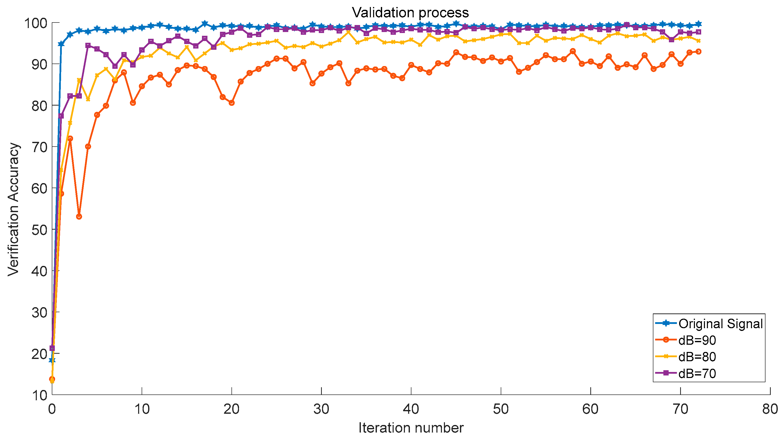
Due to the site conditions at the hydrogen refueling station and the damage to the hydrogen compressor oil pump motor bearings, we simulated the real oil pump motor bearing signals by adding 70–90 dB Gaussian noise signals and random pulse signals to the existing bearing signals. The BOA-ResNet18 algorithm has been trained to recognize signals. The results indicate that the model possesses excellent anti-interference capability, as it can still achieve over 92% training accuracy despite the presence of added noise signals. This model has practical significance.