Abstract
As a core task of computer vision perception, 3D scene understanding has received widespread attention. However, the current research mainly focuses on the semantic understanding task at the level of entity objects and often neglects the semantic relationships between objects in the scene. This paper proposes a 3D scene graph prediction model based on deep learning methods for scanned point cloud data of indoor scenes to predict the semantic graph about the class of entity objects and their relationships. The model uses a multi-scale pyramidal feature extraction network, MP-DGCNN, to fuse features with the learned category-related unbiased meta-embedding vectors, and the relationship inference of the scene graph uses an ENA-GNN network incorporating node and edge cross-attention; in addition, considering the long-tail distribution effect, a category grouping re-weighting scheme is used in the embedded prior knowledge and loss function. For the 3D scene graph prediction task, experiments on the indoor point cloud 3DSSG dataset show that the model proposed in this paper performs well compared with the latest baseline model, and the prediction effectiveness and accuracy are substantially improved.
1. Introduction
Scene understanding can simulate the human cognitive process of the natural world by perceptually recognizing various contextual information in a scene [1]. From autonomous robot navigation, autonomous driving and SLAM to AR/VR and a scene’s layout for interior design and architecture, research on scene understanding and perception is expanding in various fields [2,3]. Many studies based on 3D scene understanding have emerged, such as 3D shape classification, semantic segmentation, object detection, instance segmentation and scene layout [4,5,6]. In practical tasks, it is no longer just satisfied with obtaining simple 3D scene semantic information, such as the object and attribute information of the scene, but it also needs to obtain richer semantic relationships between objects.
A scene graph (SG) is a structured representation of objects and their attributes and interrelationships in a visual scene, where objects are represented as the nodes of the graph and relationships between objects are abstracted as edges [7,8,9]. Scene graphs based on 2D images have been applied in various scene understanding downstream tasks [10]. Due to the complexity of the object entities themselves in 3D scenes, the relevant semantic relationship features between the entities are often neglected, and there are fewer related studies on 3D scenes [11]. The scene graph structure of the semantic relationship between entities is predicted from the point cloud of the scene entities in the 3D scene graph, similar to the 2D scene graph, which abstractly represents the objects and their relationships in the 3D scene, which is due to the incompleteness of the point cloud data itself and the long-tail distribution problem of existing datasets [11,12,13,14], which has a significant impact on the prediction of 3D scene graphs. Some previous point cloud-based scene graph prediction models [11,14] directly use PointNet [4] to extract the point features and use only simple graph neural networks (GNN) [15] to infer the relationships of entities in the scene, which has substantial limitations.
In this paper, we fully consider the sparsity of scanned point cloud data and the long-tail distribution phenomenon of category annotation. We propose an improved 3D scene graph prediction model for efficient scene perception. It comprises three main network components: point cloud feature extraction and encoding, embedding prior knowledge learning and fusion, and the relationship inference of objects. The point cloud spatial coordinates of the entities in the real 3D-scanned scene are inputted to predict the scene semantic graph of the entity objects and their relationships. It expresses higher-level semantic relationships among the objects in the scene, which can be used to assist various scene understanding and perception tasks. The main contributions of this paper include the following:
- A new feature extraction coding network, MP-DGCNN, extracts multiple scales of the scene entity features from point clouds more robustly.
- The ENA-GNN was introduced to perform node and edge cross-attention in message propagation, and it improves the node-edge correlation and complex relationship prediction performance.
- The long-tail distribution of the dataset is addressed under a group-weighted scheme, including category-related embedding vectors as prior knowledge and a loss function for category balance.
- The experiments are validated, showing that the proposed model achieves state-of-the-art performance.
2. Related Work
2.1. Image-Based Scene Graph
The scene graph is a structured representation of a scene that represents the objects, attributes, and relationships between objects in the scene [10]. Classical 2D scene graph prediction methods follow a multi-stage process [10]. The first stage uses an object detection algorithm to initialize the nodes and obtain feature information, such as detection frames, visual features and categories; after that, the prediction of relational predicates that are based on object entities is performed, and this stage is a relational classification task, mainly using graph neural networks (GNNs) [16] and recurrent neural networks (RNNs) [17] to implement the inference of scene graphs. The final prediction results can be expressed as triads, such as <subject, predicate, object>. The inference ability of computers is gradually improved with the development of related technologies. Later, with the first release of the visual genome [18] dataset, a series of studies on image-based scene graph generation began to appear.
However, due to the prevalence of the long-tail distribution effects in datasets, the classification results of scene graphs can be biased when predicting the head categories and ignoring the tail categories [19]. De-biasing methods can be used to deal with this problem, such as data augmentation, resampling and re-weighting [10]. Using the Group Collaborative Learning (GCL) strategy and particular loss functions can significantly improve the average metrics of the scene graph task [20,21,22]. Furthermore, using additional prior knowledge as an effective information source can enhance the recognition of objects and inter-object relations. The knowledge-embedded routing network (KERN) implicitly incorporates co-occurrence probabilities as weights in the message propagation to eliminate the long-tail phenomenon and, thus, improves the classification performance for fewer sample categories [8]. Subsequently, Schemata first used a multi-task learning approach to encode inductive bias into prototypical features at the category level, allowing previously obtained knowledge to appear and propagate as guidance information in the perceptual model [9].
Research on the 2D scene graph is relatively mature. It has been successfully applied in various downstream scene understanding tasks, such as image understanding and inference, image retrieval, visual quizzing, caption and subtitle generation, image generation and interactive behavior detection and recognition [7,10].
2.2. 3D Scene Understanding and Scene Graph
The 3D scene understanding task requires extracting helpful information from the 3D environment, including the objects, structure and categories of entities, as well as the spatial and semantic relationships between objects. With the continuous development of point cloud deep learning, many studies on 3D scene understanding and perception have emerged, such as 3D semantic segmentation, object detection, instance segmentation and scene layout [6]. Point clouds are disordered and unstructured, and it is not feasible to use normal CNNs directly. For this reason, PointNet first considered the alignment invariance of point clouds and used a shared MLP to learn the point features and a symmetric pooling function to learn the global features, accomplishing pioneering work [4]. The later DGCNN constructs then dynamically updated the graph models in the feature space based on the point cloud space geometric features and proposed EdgeConv [5]. However, such classifications or semantic segmentation methods do not distinguish object instances. Further 3D instance segmentation tasks focus mainly on the foreground objects and ignore background elements, such as walls and floors [6]. The current point cloud-based scene understanding task still focuses on the entity object level, which cannot accurately describe the semantic relationships between objects in the scene. Further exploration is thus needed to obtain higher-level semantic information in the scenes.
With the continuous development of the field related to 3D scene understanding, the 3D scene graph has only recently started to gain attention [11]. The concept of 3D scene graphs first appeared relying on the SLAM, which dynamically builds scene graphs based on RGBD images. Furthermore, it organizes indoor 3D scenes hierarchically, dividing indoor buildings into four layers: buildings, rooms, objects and cameras, with different layers represented by tree nodes. Although such methods are hierarchical representations in 3D scenes, it is challenging to represent the more complex semantic relationships between objects [23,24,25,26]. Wald et al. first proposed the scene graph prediction network (SGPN) by using the 3D scan of a scene as input data, extracting the point cloud features using PointNet, and using GCN as a relational inference network to directly predict the structure of the scene graph in the scene point cloud, thus applying it to 3D image retrieval tasks [11]. They also published the first 3D image retrieval network based on the 3RScan dataset and released the first indoor point cloud dataset, 3DSSG, for 3D scene graph prediction tasks [11,12]. After that, based on this research, people began to improve their network structure to enhance its scene graph prediction effectively [13]. Recently inspired by Schemata [9], KSGPN learns a set of class-related meta-embedding vectors to learn class-related embeddings that avoid perceptual errors and effectively encode a priori labeled knowledge in a more distinguishable latent space [14].
The 3D scene graph can also be used for specific practical tasks, such as 3D scene retrieval, scene layout, indoor object localisation, path planning and scene captioning [11,27,28,29].
Based on previous work, this paper proposes a new model to extend the 3D scene graph prediction methods and improve the classification accuracy for the point cloud-based scene graph classification tasks.
3. Methods
3.1. 3D Scene Graph
Definition 1.
For a given 3D scene S, the goal is to generate a semantic scene graph for the 3D scene . We define the node of the instance object in the scene as that corresponds to the semantic segmentation of the instances in the scene . Each node contains the attribute class of the instance object. Relations connect the edges between nodes, and for each object-entity pair , we predict its relation predicate P, where P is the set of all possible relation predicates, such as “standing on” or “left”. Define edge , a relational triple . The relation P connects the subject and object :
Scene Graph Tasks:
(1) Scene graph classification (SGCls) predicts both the semantic categories of object entities and the semantic categories of predicates.
(2) Predicate classification (PredCls) directly predicts the semantic categories of predicates using the ground-truth labels of object entities.
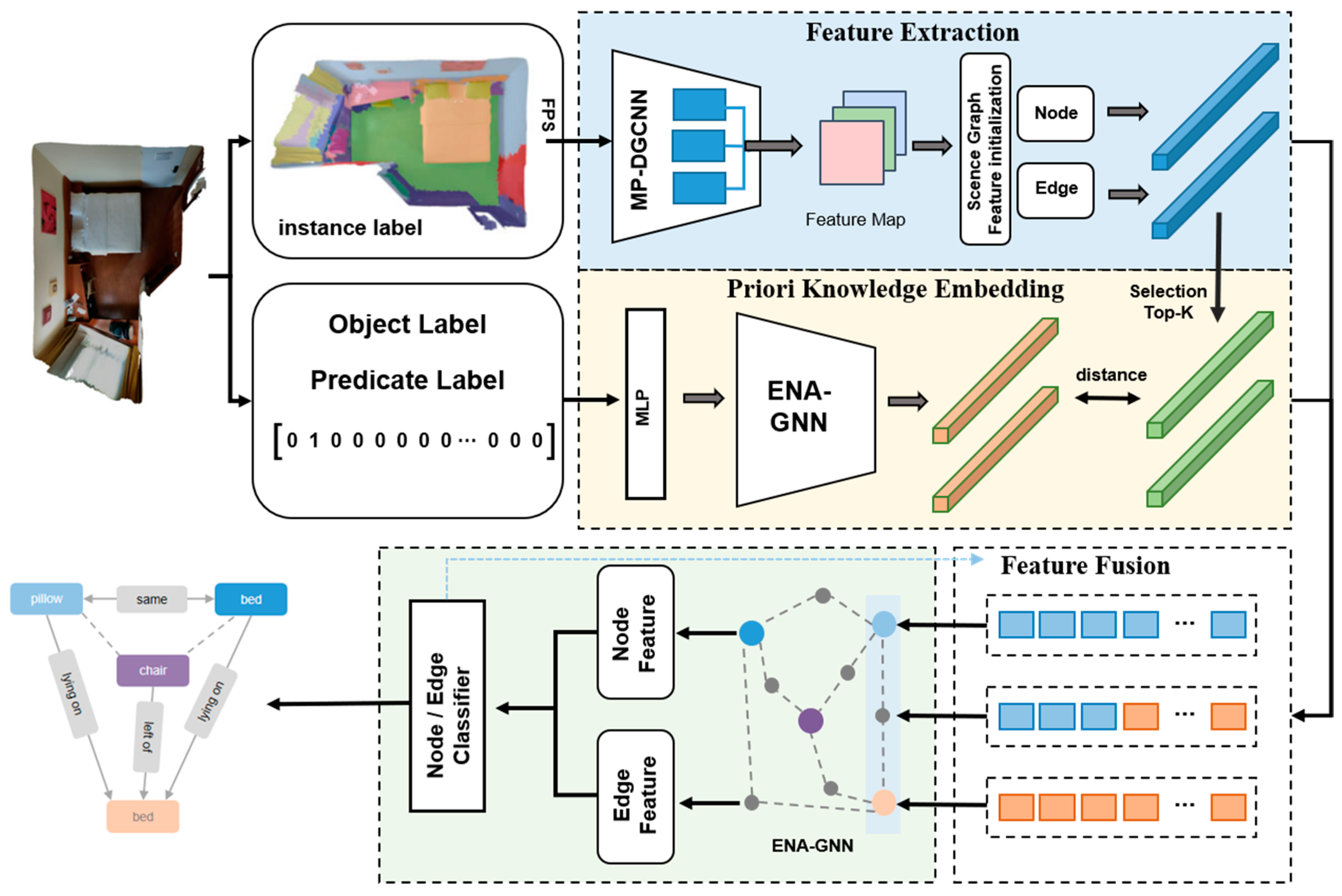
In this paper, the structure of the 3D scene semantic relationship graph prediction model is shown in Figure 1.
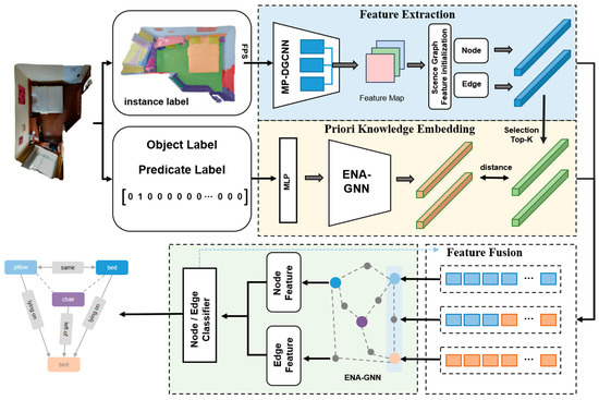
Figure 1.
Structure of the 3D scene semantic relation graph prediction model. It mainly includes point feature extraction and encoding (in Section 3.2.1), embedding knowledge learning (in Section 3.3), and relational graph inference with embedded feature fusion (in Section 3.4).
3.2. Network Design
The structure of the 3D scene graph network in this paper is shown in Figure 2, which mainly comprises scene graph feature encoding, knowledge learning, knowledge fusion and graph inference, and relationship prediction. The details of each segment’s design will be introduced in the following sections, respectively.

Figure 2.
The 3D scene graph prediction network. (a) First, enter the point cloud into the network. After MP-DGCNN extracts the initial point cloud geometric feature, , splice it with the centroid of the object, and after initialization of the node and edge features, obtain the features and . (b) Knowledge learning network stage: acquire a priori knowledge in the form of embedding vectors by learning the labels of categories in the scene and then add category weights to obtain unbiased meta-embedding (UME). (c) Knowledge fusion stage: input and , the first inference after ENA-GNN with the classifier, to obtain the initially predicted likelihood vector from the prediction results selected from the top five categories of UME and fuse them to re-run the inference process. (d) After the prediction, the scene graph triad is obtained, including objects and predicate relations.
3.2.1. Feature Extraction and Coding
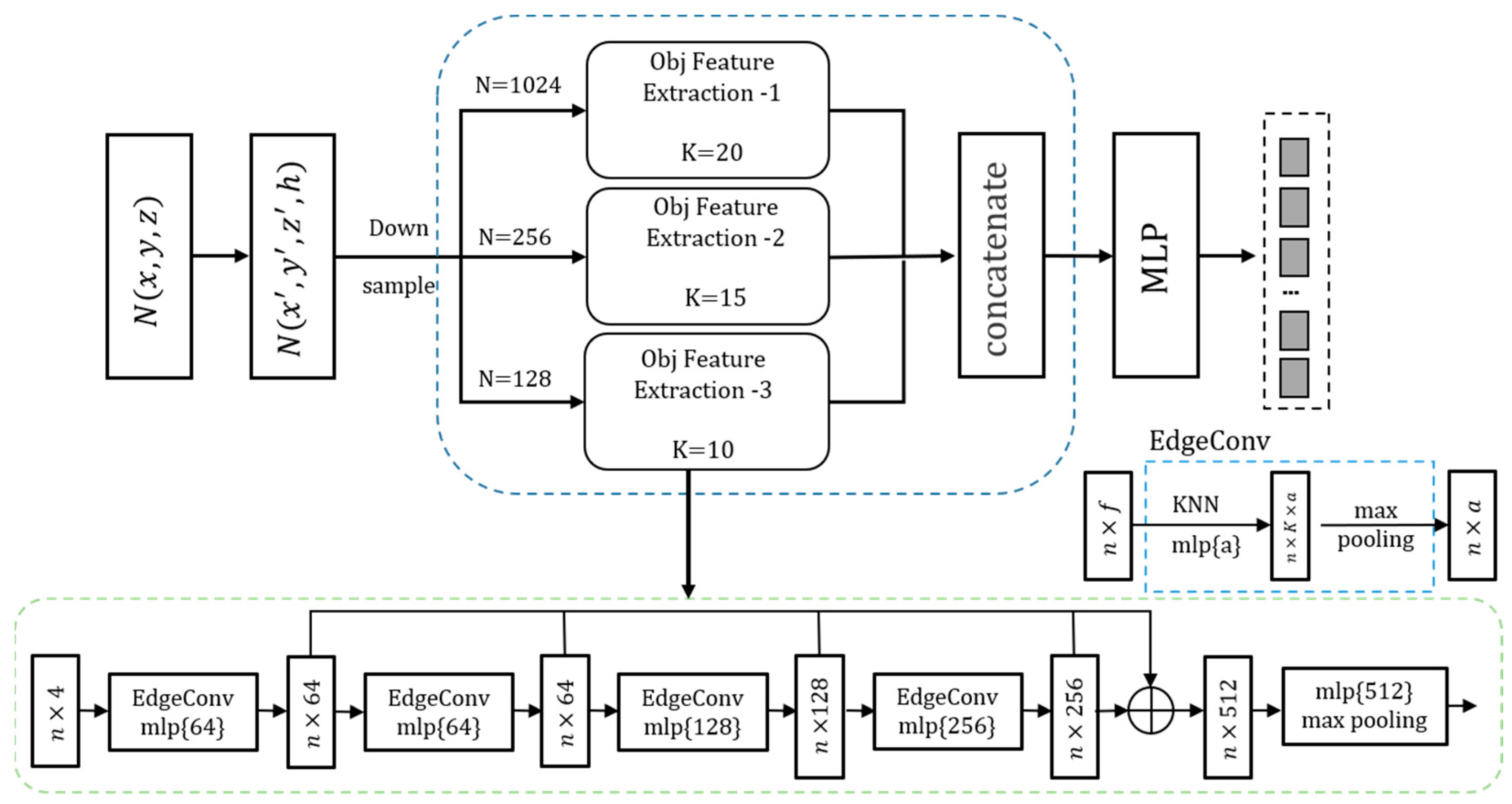
Due to the specificity of the scene graph structure, which requires encoding the features of each node and edge from the point cloud, EdgeConv using DGCNN is chosen as the core part of the feature extraction network [5]. Unlike the previous approach [11,14] that only considers using PointNet [4] for the geometric feature extraction of point clouds, EdgeConv serves as a high-performance point cloud classification model using graph theory [5]. Moreover, it can learn the point cloud’s contextual features and aggregate the neighboring information in the high-dimensional feature space. As shown in Figure 3, we added a multi-scale aggregation mechanism to the original network architecture [30,31] used to obtain the multi-scale point cloud features and thus design a new feature extraction network architecture, MP-DGCNN.
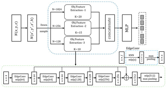
Figure 3.
Point cloud geometric feature extraction network (MP-DGCNN).
Firstly, for the M instance objects in the scene, the point cloud data is the input object. After regularization and retaining the height to obtain , the farthest distance sampling algorithm (FPS) is used for each instance object in the scene to sample the number of points N = 1024, 256, 128. The network extracts the point feature to obtain the preliminary feature map. In order to go through the following graph neural network in the relational inference, the feature initialization of the nodes and edges needs to be performed.
Node Feature Initialization: The nodes only need to go through one layer of the MLP-transformed feature space to obtain the initial node features , .
Edge Feature Initialization: The edge in the graph that represents the object node in the scene graph pointing to for each pair of objects connects the potential features with the center coordinates of the two point sets. To better encode the relative spatial relationships (e.g., left and front), the edge feature encoding method is used, which is initialized using the concatenate scheme as follows:
where refers to the concatenate of the feature vector, after which the feature space is transformed to the same feature dimension as the node by MLP to obtain the initial edge embedding feature .
3.2.2. ENA-GNN: Node and Edge Cross-Attention
Some global relational inference methods for GNNs have recently emerged [13,32,33,34,35] that apply GCNs [16] for node-wise message propagation to obtain their evolved node features based on graph-based reasoning [10]. Our model is inspired by graph-wise message propagation and graph-based reasoning to obtain the evolved node features and apply them to the scene graph tasks [36]. This paper is inspired by these methods and uses the gate recurrent unit (GRU) [37] to deliver the node and edge messages layer by layer. Moreover, node and edge cross-attention are added to the message delivery process to propose the ENA-GNN network (Figure 3). ENA-GNN can realize joint graph inference and node classification prediction of a 3D scene graph node and edge features. The graph inference network is mainly deployed in the prior knowledge learning process with the final inference process of the 3D scene graph.
As in Figure 4, at the level of the graph neural network design for relational inference, we adapted the message-passing mechanism to a directed graph structure [37,38], combined with the edge cross-attention mechanism [13] where and are the edge cross-attention score and the node cross-attention score, respectively.

Figure 4.
SGConv of fused nodes and edge cross-attention: the complete ENA-GNN includes multiple layers of SGConv.
- (1)
- Node Feature Fusion Edge Attention.
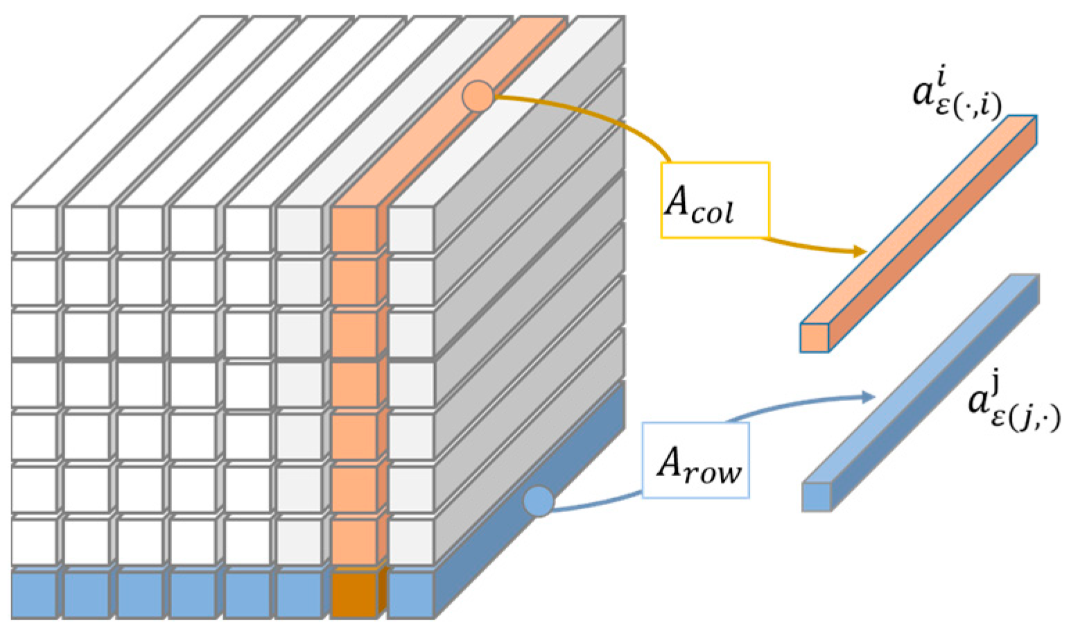
To make better use of the edge information, as shown in Figure 5, for one of the nodes in the graph ; by considering the node as the SUBJECT or OBJECT in various edge relationship connections, respectively, for , calculate its edge interaction vector . The node , received by the interaction signals of , and the node received by node are aggregated and represented by the edge indexes as and :

Figure 5.
Edge cross-attention, incorporating edge features.
The is a neural network transformation matrix, and and denote the channel aggregation functions executed along the row direction and column direction, respectively. Thus, as shown in Figure 5, the overall edge cross-attention to node V, and the attention score to one of the elements can be expressed as:
where ⊙ stands for the Hadamard product and denotes the nonlinear activation function.
- (2)
- Edge Feature Fusion Node Attention.
Similarly, after the network messaging at the current layer, the feature information between nodes through another node cross-attention simulates the interaction, and the is configured on the edge after the message-passing process on the . For the two nodes and and the directional edge , the potential feature and of the corresponding node can be determined by an edge to obtain their node cross-attention score , which is calculated as follows:
where and represent the learnable weight matrices and are also used to transform the node features to the same number of channels. Furthermore, and denote the nonlinear activation functions.
- (3)
- Message Propagation.
For the core layer of ENA-GNN, each layer of the network messaging is partly based on the connection relationship between the nodes. In the triad (subject, predicate and object) of the scene graph inference, the features of , respectively, are connected according to the index of the subject and object, corresponding to the nodes and to obtain the potential features of and . The initial message is passed through the following feature message encoding [11,14]:
For the , the message-passing process is calculated as follows:
where , and are the three nonlinear transformation MLPs with different dimensions as the subject, predicate and object, respectively. Feature layer normalization (LN) [39] is used to smooth the computational process of message transfer after feature fusion, and is the preliminary encoded message.
After that, the message of node V is characterized by , which is the node used as the subject and object, respectively:
where |∙| denotes the base (calculated quantity), and the and are the sets of connections of node v as the subject and object, respectively.
Eventually, a gated recurrent unit (GRU) [37] is used to update the hidden state to retain the initial information. In order to calculate all nodes in each layer and all directed edges of the potential representations and of the message-passing process, the message propagation of the nodes and edges is as follows:
where ⊙ denotes the Hadamard product for interacting with the cross-attention of nodes and edges with the obtained information of this layer. denotes a layer of gated recurrent network units for feature message delivery and updates.
3.3. Unbiased Meta-Embedding
In 3D scene graph prediction, a meta-embedding knowledge learning model [14] is used to learn the a priori knowledge obtained from the ground-truth one-hot code of the training set as common categories knowledge. It considers only the class-related labels without considering the visual perceptual information and then fuses the multi-source features and information in the final graph inference process. In training, we initially assume that there is a relationship between each entity object before organizing the objects and relationships into a graph structure, where the objects are represented as nodes and the predicate relationships are represented as edges. In terms of the network structure, a multi-layer perceptron (MLP) is used to raise the label vector to the same feature space as the point feature encoding vector. Then, an ENA-GNN network is used to enable the feature aggregation and message updates for each node and edge in the scene graph.
As in Figure 2, the GT labels are used as network inputs, and the meta-embedding (ME) vector is first initialized, where , n is the number of object categories or relational predicate categories, and C is the feature dimension. During the knowledge learning process, the meta-embedding vector is iteratively updated by continuously closing the gap between the embedding vector and the potential feature vectors. The deviation distance of the two vectors is used as a loss function and is back-propagated [40].
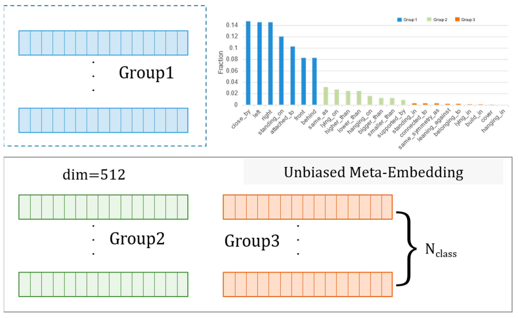
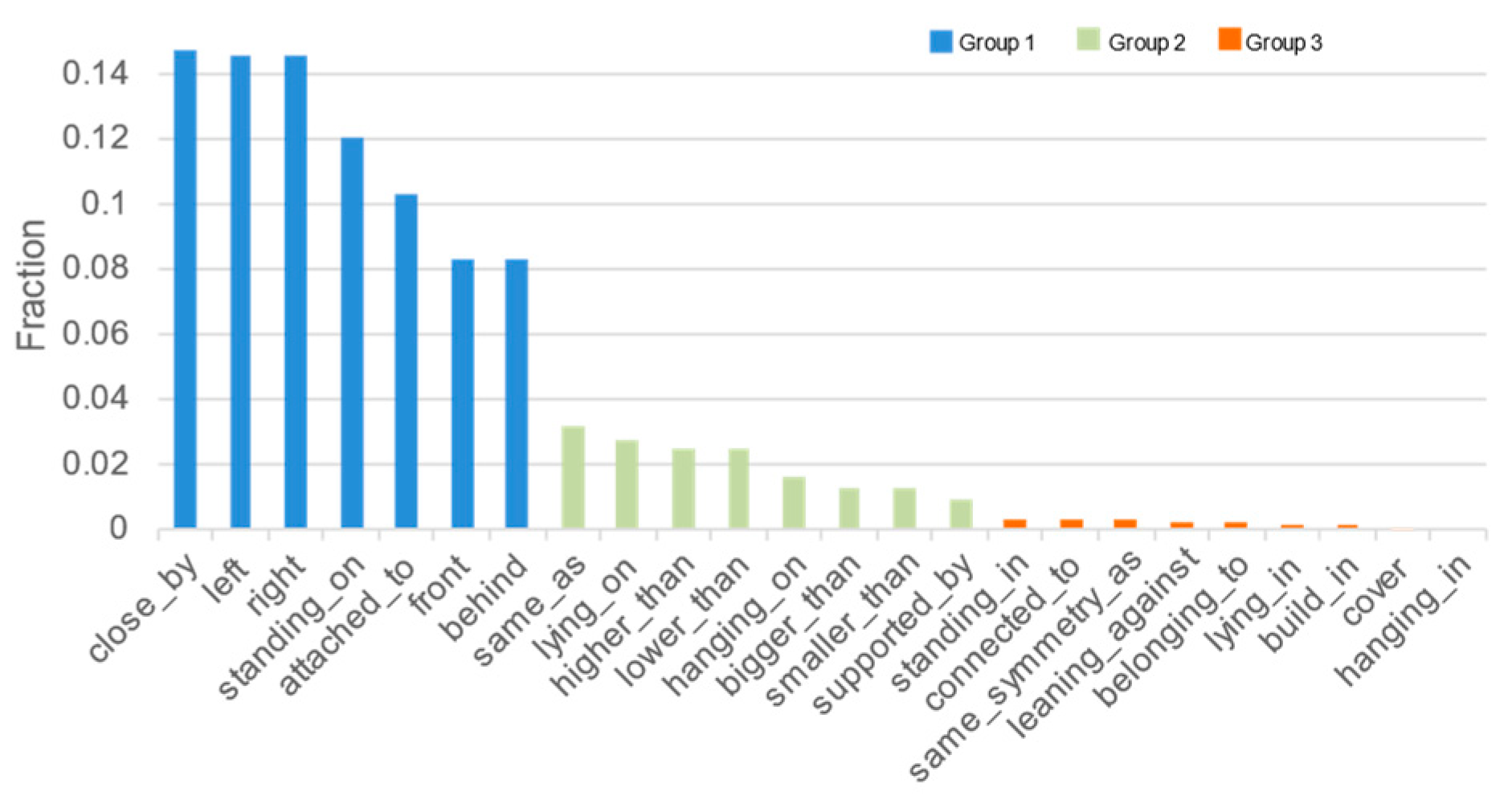
However, the learned meta-embeddings as a priori knowledge are unclear and may interfere with the network model category prediction [14]. Based on the idea of unbiased training, an unbiased meta-embedding (UME) coding fusion approach is proposed to group the predicate relation categories in order of sample proportion. As seen in Figure 6, the categories are divided into three groups, and the detailed grouping strategy is referred to in Section 4.1.
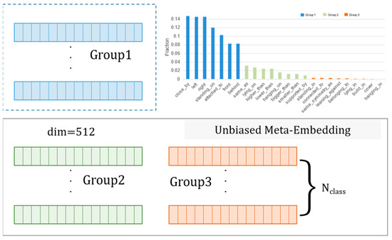
Figure 6.
Grouping relationship categories by frequency and reducing the weight of common relationship category meta-embedding in the feature embedding fusion process to obtain unbiased meta-embedding.
In KSGPN [14], it is known from the existing experiments that the embedding knowledge of category labels can guide the network to make more balanced predictions of relational categories. However, for the common relational categories, it may be noisy, thus affecting the accuracy of the common predicate relational categories (in Group 1). Therefore, for the common categories, we reduced the proportion of prior knowledge weights for the high-frequency samples (Group 1) in the relational inference process to avoid the formation of excessive irrelevant noise effects. For the samples with a relatively low frequency of occurrence (Groups 2 and 3), their prior knowledge encoding is retained to obtain unbiased meta-embedding encoding (UME).
3.4. Scene Graph Relational Reasoning
In the relational inference process of the scene graph, as shown in a part of Figure 2, after the initialization of the node and edge features, the initial potential features are obtained. This is then fused with the label category’s prior knowledge, i.e., unbiased meta-embedding prior knowledge (UME), and the relational inference is performed by the ENA-GNN network to obtain the object and relational feature encoding, respectively. Finally, the category is obtained using fully connected layer (FC) prediction.
The knowledge fusion process, divided into multiple iterative loop processes, can be carried out several times using the knowledge fusion process. Firstly, for the knowledge selection, the object and predicate category probability vectors can be obtained after the initial prediction of the scene graph. The corresponding features of the predicted category with a top-five likelihood are selected for fusion. The category selection is carried out for the meta-embedding encoding, as seen in Figure 7, and the category’s prior feature vector after the screening is obtained. The selected prior embedding UME is fused with the extracted point features. Since they are in different feature spaces, they are transformed into approximate feature spaces using two layers of encoded feed-forward neural networks, f (∙) and g (∙) [14]:

Figure 7.
Unbiased meta-embeddings as prior knowledge and the corresponding unbiased meta-embeddings of the top-five likelihood prediction categories are selected for fusion.
We used to denote the selected meta-embeddings, to denote the grouping of relationship categories with weights, and is a two-level MLP.
3.5. Loss Function
Due to the common phenomenon of long-tail distribution in the scene graph dataset, the sample distribution differs significantly between different categories, and the choice of using focal loss [41] is considered as the classification loss function, as follows:
where p is the logarithm of the object or relation predicate prediction, and α and γ are hyperparameters, where γ is set to 2. The parameter settings refer to the existing model settings [11,14], where is a category weight, which is the normalized inverse frequency of each category in the object classification.
In particular, for the predicate classification, inspired by the equalized focal loss (EFL) [42], the idea of using an improved balanced focal loss (BFL) is as follows:
where the category balance weights are added to the above equation focal loss, and α is used to distinguish between the edged and unedged connections in the predicate classification, where α is set to 0.25 and 1, respectively; however, for the partial zero-sample category existing in the dataset, α is set to 0. Additionally, where , is the different category balance weights, and the group re-weighting is performed for different predicate relation categories; see Section 4.1 for the detailed group re-weighting details.
In the scene graph prediction task, the prediction results include object categories with relational triples . The loss function is defined as follows:
where according to the triple properties, set = 0.5, the object category predictions are weighted. In addition, the loss function uses the Euclidean distance between the latent vectors of each category and the meta-embedding vectors. The L2-norm is, therefore, the loss in the meta-coding knowledge learning process [14]:
where and are the corresponding meta-embedding vectors of the node, V, corresponding to the entity object and the edge, E, corresponding to the object relation. In the meta-embedding learning task, the loss function can be formulated as follows:
4. Experimental Section
4.1. Experiment Preparation
Implementation Details: The experiments were conducted using the deep learning frameworks Pytorch 1.9.0, Python 3.8 and Cuda 11.1, and the operating system Ubuntu 18.04. The training was completed on a device with AMD R-5800H and 16 GB RAM on an 8 GB NVIDIA GeForce RTX3070 laptop, following the same parameter settings as the baseline model using the following: Adam optimizer; fixed random seeds; an initial learning rate set to 0.0001; a decay of 0.7 per 10 epochs; batch size set to 1; epoch set to 40 and using the early termination strategy. All models were trained on the same dataset as the 3DSSG dataset.
Dataset: The 3DSSG, a publicly available large indoor 3D semantic scene graph dataset, is based on the realistic 3D scan dataset, 3Rscan [11,12]. The dataset mainly contains support, proximity and comparison relationships between the entity objects in indoor scenes. During the training process, larger scenes are partitioned, with an average of 9 objects per scene, 160 classes of entity objects and 27 classes of relationships between objects (including “none”). The training file is divided so that there are 3582 scenes in the training set and 548 in the validation set.
Dataset Preprocessing: The original dataset has incomplete 3D-scanned scenes and a small number of annotation errors, and the dataset has severe long-tail distribution problems. We performed preprocessing operations on the dataset and group statistics of the categories for subsequent experiments.
The following preprocessing operations were completed for each scanned split in the dataset to reduce the training data preprocessing times:
- Obtain the instance IDs in each scene from the dataset and establish the mapping relationship with the corresponding point cloud.
- Conduct sampling by the farthest point sampling (FPS) algorithm, sampling 1024 coordinate points per object instance on average and using random sampling to complement the small target entities to align the training data.
- Using the ground-truth labels, remove some of the individual scenes cut that do not contain relationships or entities, count the frequency of each category and sort them, and remap the labels of each category.
- Save the scene point cloud and label the array files to a separate folder under each scene, and generate the training set and validation set files.
Group Weighted (GW): For the long-tail distribution phenomenon, the predicate categories are grouped according to the sample distribution in the dataset [20].
The grouping results are shown in Figure 8, where different object entities and predicate categories are statistically sorted according to the number of samples. The grouping principle is the extreme difference in the number of samples of different categories within the group that does not exceed 4 times. For the weights in the training process allocation, this paper uses a weighting approach, and for each group of categories, a weight range is set and calculated as follows:
where is the number of samples in each category, is the total number of samples in each group, and f (∙) is the normalization method that maps the range to [0, 1]. The first group sets the weight range [0, 0.25], which is reverse-weighted according to the number of samples in each category in the group; the second group sets the range [0.5, 1] using the same steps; the third group, which is small sample categories, all take 1.
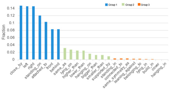
Figure 8.
Predicate category grouping results.
4.2. Evaluation Metrics
Several recall metrics (R@K) are mainly used to evaluate the model’s performance for the two types of tasks, SGCls and PredCls, of the scene graph, and K = 20, 50, 100 are taken for evaluation.
R@K [43]: Recall@K is a widely used metric in scene graph tasks to calculate the recall of the top-n for each model prediction triad (s, p, o). Triads are correctly predicted only when the subject, predicate and object are correctly predicted.
ngR@K [44]: In the traditional recall calculation, only one relationship category of a pair of objects can participate in the final calculation; however, ngR@K allows all relationship categories (relationships) of a pair of objects to participate in the sorting.
mR@K [45]: For Mean Recall@K, due to the long-tail phenomenon of category labeling in the dataset, the mean recall is considered for evaluating the prediction performance of the model for the non-uniformly distributed categories. The mR@K calculates the recall for all the predicate categories separately and then calculates the mean value, which can fully account for the importance of all the categories and will be relatively more informative.
4.3. Baseline Models
Some of the 2D scene graph methods using a priori knowledge and existing 3D scene graph generation frameworks were selected as the baseline models. We compared them mainly with the best-performing baseline models, where the same training environment and parameter settings were used for the experiments on irrelevant factors.
SGPN [11]: A scene graph prediction network was proposed—the first end-to-end network for point cloud 3D scene graphs. The SGPN uses two parallel PointNets for feature extraction to obtain the object and edge features and uses the GCN for the relational inference.
Priori knowledge-based methods [8,9]: KERN and Schemata are 2D scene graph methods that use a fused prior knowledge approach. In the experiments, in order to facilitate comparisons with the 3D scene graph method, PointNet was used directly to replace the image feature extraction module in the original model. Such methods were introduced into the 3D scene graph task as a baseline model for comparison. Among them, the knowledge-embedded routing network (KERN) represents the statistical correlations between the objects appearing in the image. Their relationships are explicitly demonstrated using a structured knowledge graph and prior knowledge. Schemata first proposed the idea of prior knowledge learning to learn a set of weighted feature vectors associated with a category.
KSGPN [14]: As the best baseline model so far, referring to the ideas of KERN and Schemata, based on SGPN, this method of fusing prior knowledge into a 3D scene graph prediction task was used for the first time. It proposes that prior encoding knowledge and the embedding vectors’ fuse point cloud features significantly improve the prediction effect of the 3D scene graph.
4.4. Experimental Results and Analysis
The experiments are compared using the official 3D scene scan split strategy of the 3DSSG dataset.
Comparison experiments were conducted with other baseline models and compared with the current best-performing a priori knowledge-based 3D scene graph approach. Table 1 and Table 2 show that our model has significantly improved its prediction on the 3D scene graph task, achieving the best relationship recall on both SGCls and PredCls tasks and the best model performance. Furthermore, there is a significant improvement in mR@K, which indicates that our method can mitigate the effect of long-tail distribution. Therefore, our method has a better prediction effect for the less sample category.

Table 1.
Results of quantitative analysis of SGCls for the scene graph classification task (in %, inclusive standard deviation and bolded for best performance).

Table 2.
Predicate classification. (in %, inclusive ± standard deviation and bolded for best performance).
Table 1 compares our model with other models in the scene graph classification task. Our proposed method improves the recall significantly on the scene graph classification task by about 23.6% and 24.2% under the R@50 and ngR@50 metrics, respectively, and by about 18.2% under the mR@50 metric. As shown in Table 1, the experiments also validate the experimental effect of KSGPN [14] under the GW grouping re-weighting training strategy proposed in this paper. We added weights to different grouping categories and used the grouped meta-embedding features, UME. We can see that the prediction effect is also improved significantly by about 3.1% under the mR@50 metric compared to the original model.
In the scene graph classification task, the object category’s correctness significantly impacts the result. The more significant improvement, when compared with the baseline model, might be because we used a better point cloud feature extraction and encoding model. In order to verify this idea, as shown in Table 3, we conducted a comparison experiment on the different point feature extraction parts of the model and trained this part separately, and then directly used the fully connected layer to predict the object and predicate categories. Compared to the baseline model, MP-DGCNN has more robust feature extraction and coding capabilities. The results are significantly improved for object classification, and the improvement in the mean accuracy index is noticeable, which is beneficial for the subsequent prediction of small sample categories.

Table 3.
Comparison results of object coding modules (in % and bolded for best performance). Training the point cloud feature extraction and encoding network alone and using MLP directly as a classifier with other training parameters unchanged, such as the MP-DGCNN. Our point feature encoding network for scene graphs is compared with the KSGPN [14].
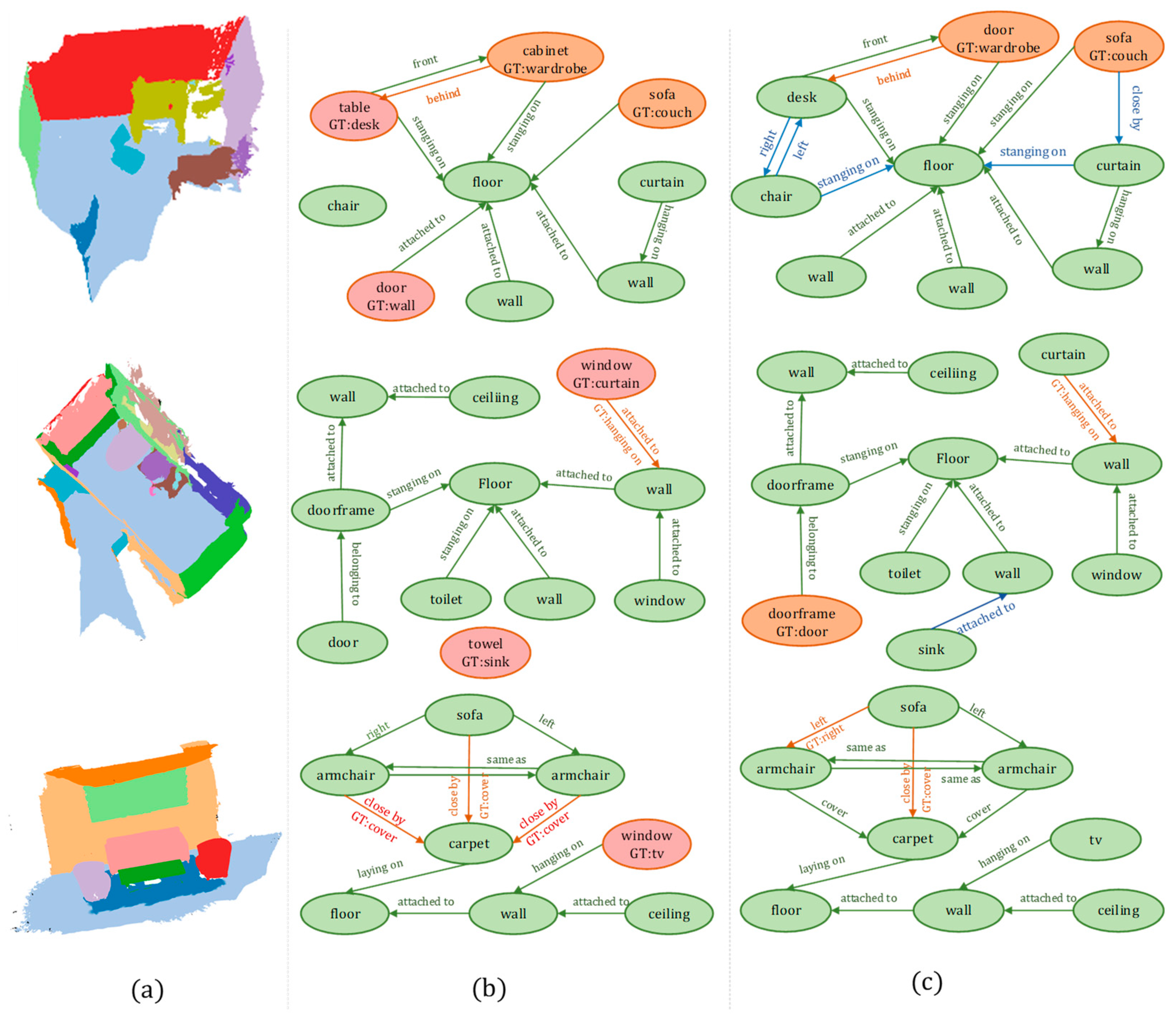
The visualized qualitative results of the scene graph classification (SGCls) are shown in Figure 9. Compared with the baseline model, KSGPN, our model outperforms the baseline model regarding object recognition and relationship inference, such as “wall-door” and “tv-window”, which are confusingly similar objects. Our model can also infer the correct relationship between some isolated entities, which do not exist with other entities in the ground-truth labels, and the surrounding objects.
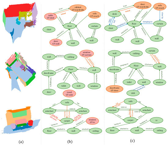
Figure 9.
Visual qualitative results of scene graph classification (SGCls). Where the results with wrong or ignored predictions are shown in red, the results with correct predictions are shown in green, and the results with reasonable inferences with correct predictions but unlabeled true labels are shown in blue. Where (a) shows the instance segmentation mask of the scene; (b) shows the KSGPN [14] for the scene graph prediction and explicitly distinguishes the results with incorrect predictions for similar objects; (c) is the prediction results for our model.
Table 2 shows the results of the predicate classification task. In the predicate classification task, the category for the object is known information; therefore, improving the prediction effect is mainly related to the relational inference network and the use of prior knowledge. The effect of the feature extraction by MP-DGCNN is weakened in this task. However, the relational inference network, ENA-GNN, used in our method, enhances the adaptive capability of message-passing in graph neural network inference by taking into account the cross-attention of the nodes and edges; at the same time, the loss function is weighted by group re-weighting (GW) and incorporates the UME a priori category knowledge coding. The experimental results show that the method proposed in this paper still significantly improved when compared with other baseline models, including the latest methods. The prediction results improved by about 3.4% and 5.9% under the R@50 and ngR@50 metrics, respectively, and about 1.5% under the mR@50 metric by about 1.9%. The results improved by about 7.6% and 10.3% under the R@20 and ngR@20 metrics, respectively, and by about 7.6% under mR@20.
In addition, our proposed model takes more time in each epoch of training time; however, the convergence speed is improved, taking about 16–18 h to train and about 13–15 h for the baseline model, KSGPN [14]. Because of the use of a more robust feature extraction network, there is an increase in network complexity.
To summarize the experimental process and results, our approach starts with point cloud feature extraction and initial coding using MP-DGCNN. During the training process, different categories in the loss function are re-weighted, and the meta-embedding vector is similarly grouped and weighted to obtain unbiased meta-embedding during the knowledge fusion process. Our model is compared with the baseline model for experiments, and various quantitative metrics showed significant performance improvements in the scene graph tasks. The experiments demonstrate that our model can better extract point cloud features. For the relational inference process, a cross-attention mechanism of nodes and edges is added to improve the robustness and inference capabilities of the network.
4.5. Ablation Experiments
Some improvement strategies of this paper are verified in their effects, respectively. In order to verify the influence of each section on the final results, we compare the experimental effects of the model after adjusting or removing a particular module. We then verify the results on the scene graph’s two tasks, SGCls and PredCls.
4.5.1. Model Design
Some of the main modules are as follows:
ENA(ENA-GNN): The introduction of node and edge cross-attention in the original GNN messaging process to enhance the relevance of the nodes and edges in relational reasoning.
GW: Group re-weighting for different categories, using focal loss function while considering category equilibrium, aims to improve the prediction effect of low-frequency categories with few samples.
UME: The unbiased meta-embedding vectors, which are obtained from category label learning, are grouped according to the sampling ratio of the categories, and their weights are reduced in the knowledge fusion process for the group where the common categories are located in order to avoid interfering with the training of the common categories.
MP(MP-DGCNN): A new point feature extraction and encoding network model with multi-scale-sampled point clouds, combined with a pyramid structure to jointly extract the multi-level geometric features of point clouds and improved initialization of the edge features.
Table 4 shows the ablation tests of the different network parts of the model with the training strategy. From the experimental results, we can conclude that the model approach proposed in this paper has the best overall effect for the final experiment. Among them, MP-DGCNN has the most apparent overall improvement in the scene graph task (SGCls). It shows that the point feature extraction network is critical for the 3D scene graph prediction task and will directly determine the accuracy of the subsequent relational inference. In the predicate classification task, the ground-truth labels of the objects are known, and MP-DGCNN only encodes the feature of the edges, which has a weak impact on the final experimental results. While using the re-weighting group strategy will significantly improve the mR@K, which can alleviate the phenomenon of the long-tail distribution of data and balance the prediction effect of different grouping categories. Nevertheless, it accordingly decreases the R@K and ngR@K slightly, i.e., there is an inevitable negative impact on the overall prediction.

Table 4.
Results of ablation experiments of SGCl-PredCLs (each module is removed separately, and the experimental results are observed using percentages % of results, bolded for best performance and underlined for secondary performance).
4.5.2. Point Cloud Data Dimension
The validation model additionally uses the normal vectors of the point cloud as features, and the experimental results are shown in Table 5. However, the experimental performance in the scene graph classification (SGCls) task is slightly better in the R@K and ngR@K indexes than the model using only the point cloud coordinates. However, all other indexes, especially in the mean Recall@K, are descending, and the complexity and running time of the model are substantially increased.

Table 5.
Results of each prediction using the normal vector of the point cloud in the extraction stage of point cloud features (in % and bolded for best performance).
Therefore, only using the point cloud coordinate information to extract the features in the scene graph classification task is recommended, which is the most cost-effective.
4.5.3. Knowledge Integration Iterations
In the final stage of the model, the node and edge features obtained from initialization are used for the knowledge selection and fusion with the unbiased meta-embedding vectors in the graph inference part. This is an iterable process, as shown in Figure 10 below. The number of iterations for embedding knowledge fusion is adjusted separately in the predicate classification task. The model is most cost-effective regarding the running time and performance when t = 1, i.e., only one embedding vector selection and one knowledge fusion process are performed.
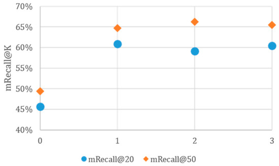
Figure 10.
Adjusting the number of iterations in the knowledge fusion process, using mRecall@20 and mRecall@50 for evaluation.
4.5.4. Weakly Supervised Ablation Tests
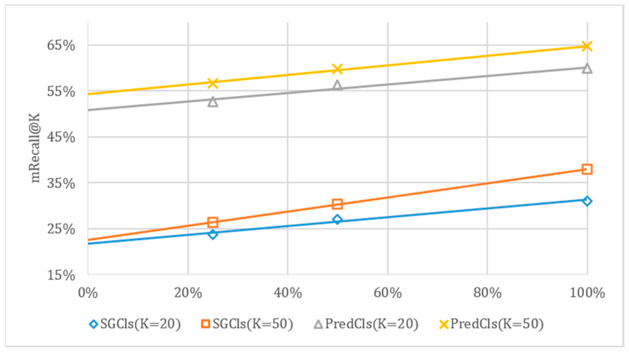
Since the prior embedding vectors from the ground-truth labels’ learning are used, our ENA-GNN network can better fuse the prior embedding vector features with the extracted initialized point features. Figure 11 shows the experimental results using different proportions of the training set samples. We can obtain similar experimental results to the full sample participation using about half of the training samples. Since, for the PredCls task, the ground-truth labels of the objects are known, acceptable predicate classification results can be obtained with a tiny number of samples involved in the training.
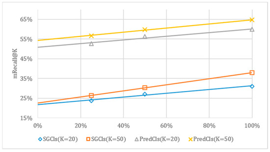
Figure 11.
Training results with reduced training set sample proportions were evaluated using mRecall@20 and mRecall@50.
4.5.5. The Impact of Each Module of the Long-Tail Distribution Is Considered
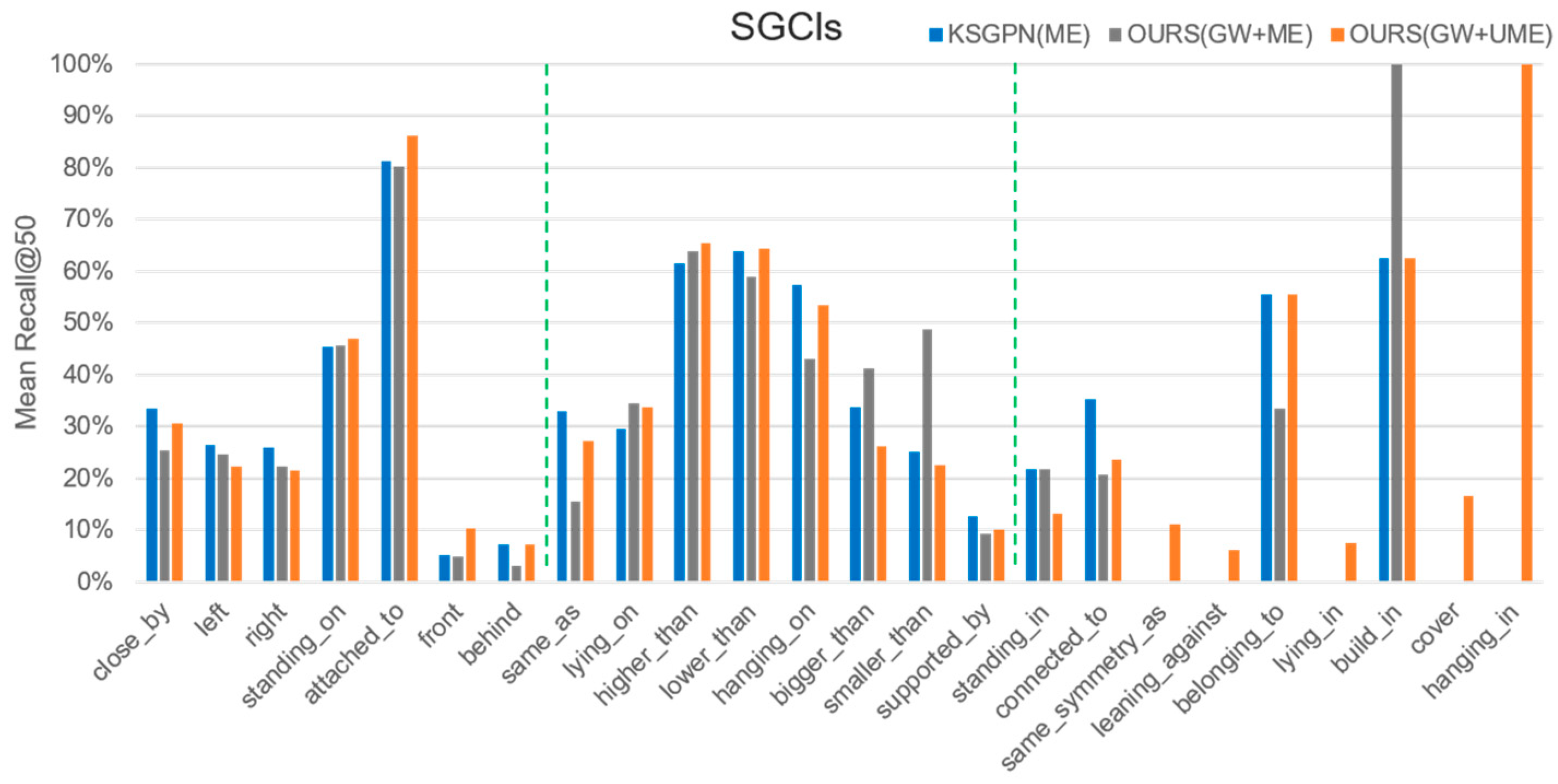
In order to understand the importance of grouping re-weighting with fused unbiased prior knowledge for the prediction of few-sample categories, we conducted ablation tests on the prediction results of different predicate categories. We performed statistical comparisons of the experimental results. Figure 12 and Figure 13 show the experimental parameter results of the scene graph classification (SGCls) and predicate classification (PredCls) tasks for a single category, respectively. It can be seen that using group re-weighting (GW) alone performs poorly in the common category (Group1), which significantly affects the overall mRecall@K performance. Meanwhile, the combined use of the GW strategy with UME, as prior knowledge vectors perform better overall than the KSGPN network using ME alone in the common categories, with little degradation in precision, especially for the tail categories, yields better prediction results.
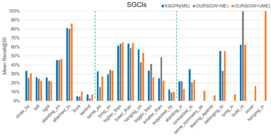
Figure 12.
Experimental results for each category of the scene graph classification (SGCls) task, with categories listed from left to right according to the statistical frequency of the samples. Comparisons are made using our method (GW + ME) and our method (GW + UME) with KSGPN (ME).
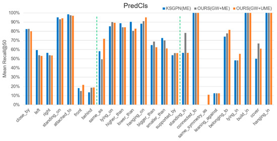
Figure 13.
Experimental results for each category of the predicate classification (PredCls) task, with categories ordered from left to right according to the statistical frequency of the samples. Comparisons are made using our method (GW + ME) and our method (GW + UME) with KSGPN (ME).
5. Conclusions and Discussion
This paper proposes a 3D scene graph prediction model for efficient environment perception, focusing more on predicting the semantic graph about the class of entity objects and their relationships. MP-DGCNN is proposed for more robust feature extraction, and ENA-GNN is introduced to infer complex relationships. A category grouping weighting strategy was attempted to solve the problem of the long-tailed distribution of datasets. Our model was validated on the 3DSSG dataset and achieved state-of-the-art performance. The research in this paper contributes to various tasks related to understanding 3D scenes for indoor autonomous robotic applications.
However, the FPS algorithm samples the point cloud and the multi-scale pyramidal network structure in the point feature extraction process. Although the point cloud features can be aggregated well, the time cost increases. More efficient sampling and point feature aggregation algorithms can be found in the future. Furthermore, due to the limitations of the available public datasets and the unbalanced distribution of the category annotations, the current approach relies, to some extent, on the dataset’s completeness. It is currently limited to predicting indoor scenes and needs to be explored more deeply in more complex scenes, such as outdoor and dynamic scenes.
In future work, considering the expansion of indoor and outdoor scenes and downstream application fields, future research can rely on the SLAM algorithms combined with real-time dynamic point cloud instance segmentation and 3D object detection, and other deep learning technologies. The ultimate expectation is to achieve dynamic predictions and generations of indoor and outdoor scene graphs. It is expected to be applied to robotic scene understanding tasks, thus extending the AR/VR domain and aiding the interactive perceptual behavior of intelligent agents within.
Author Contributions
Conceptualization, methodology and writing—original draft preparation, C.H.; data curation, C.H. and Y.W.; supervision, project management, fund acquisition and resources, S.Z. and H.L.; software and validation, C.H., B.D. and J.X.; investigation, C.H., X.Z., S.Z. and H.L.; visualization, writing—review and editing, C.H., H.L., Y.W. and X.Z. All authors have read and agreed to the published version of the manuscript.
Funding
This research is supported by the key project of the National Natural Science Foundation of China—“Machine Map Theory and Modeling Method”, with support number 42130112.
Informed Consent Statement
Not applicable.
Data Availability Statement
Data can be obtained from the corresponding author upon reasonable request.
Acknowledgments
The author would like to thank those who contributed to the model and dataset open sources. At the same time, we thank the editors and reviewers for their valuable comments.
Conflicts of Interest
The authors declare no conflict of interest.
References
- Fei-Fei, L.; Koch, C.; Iyer, A.; Perona, P. What Do We See When We Glance at a Scene? J. Vis. 2004, 4, 863. [Google Scholar] [CrossRef]
- Tahara, T.; Seno, T.; Narita, G.; Ishikawa, T. Retargetable AR: Context-Aware Augmented Reality in Indoor Scenes Based on 3D Scene Graph. In Proceedings of the 2020 IEEE International Symposium on Mixed and Augmented Reality Adjunct (ISMAR-Adjunct), Recife, Brazil, 9–13 November 2020; pp. 249–255. [Google Scholar]
- Luo, A.; Zhang, Z.; Wu, J.; Tenenbaum, J.B. End-to-End Optimization of Scene Layout. In Proceedings of the IEEE/CVF Conference on Computer Vision and Pattern Recognition, Seattle, WA, USA, 13–19 June 2020; pp. 3754–3763. [Google Scholar]
- Charles, R.; Su, H.; Kaichun, M.; Guibas, L.J. PointNet: Deep Learning on Point Sets for 3D Classification and Segmentation. In Proceedings of the 2017 IEEE Conference on Computer Vision and Pattern Recognition (CVPR), Honolulu, HI, USA, 21–26 July 2017; IEEE Computer Society: Los Alamitos, CA, USA, 2017; pp. 77–85. [Google Scholar]
- Wang, Y.; Sun, Y.; Liu, Z.; Sarma, S.E.; Bronstein, M.M.; Solomon, J.M. Dynamic Graph Cnn for Learning on Point Clouds. ACM Trans. Graph. 2019, 38, 146. [Google Scholar] [CrossRef]
- Guo, Y.; Wang, H.; Hu, Q.; Liu, H.; Liu, L.; Bennamoun, M. Deep Learning for 3D Point Clouds: A Survey. IEEE Trans. Pattern Anal. Mach. Intell. 2021, 43, 4338–4364. [Google Scholar] [CrossRef]
- Johnson, J.; Krishna, R.; Stark, M.; Li, L.-J.; Shamma, D.; Bernstein, M.; Fei-Fei, L. Image Retrieval Using Scene Graphs. In Proceedings of the IEEE Conference on Computer Vision and Pattern Recognition (CVPR), Boston, MA, USA, 7–12 June 2015. [Google Scholar]
- Chen, T.; Yu, W.; Chen, R.; Lin, L. Knowledge-Embedded Routing Network for Scene Graph Generation. In Proceedings of the IEEE/CVF Conference on Computer Vision and Pattern Recognition (CVPR), Long Beach, CA, USA, 15–20 June 2019. [Google Scholar]
- Sharifzadeh, S.; Baharlou, S.M.; Tresp, V. Classification by Attention: Scene Graph Classification with Prior Knowledge. Proc. AAAI Conf. Artif. Intell. 2021, 35, 5025–5033. [Google Scholar] [CrossRef]
- Chang, X.; Ren, P.; Xu, P.; Li, Z.; Chen, X.; Hauptmann, A. A Comprehensive Survey of Scene Graphs: Generation and Application. IEEE Trans. Pattern Anal. Mach. Intell. 2022, 45, 22359232. [Google Scholar] [CrossRef] [PubMed]
- Wald, J.; Dhamo, H.; Navab, N.; Tombari, F. Learning 3d Semantic Scene Graphs from 3d Indoor Reconstructions. In Proceedings of the IEEE/CVF Conference on Computer Vision and Pattern Recognition, Seattle, WA, USA, 13–19 June 2020; pp. 3961–3970. [Google Scholar]
- Wald, J.; Avetisyan, A.; Navab, N.; Tombari, F.; Niessner, M. RIO: 3D Object Instance Re-Localization in Changing Indoor Environments. In Proceedings of the IEEE/CVF International Conference on Computer Vision (ICCV), Seoul, Republic of Korea, 27 October–2 November 2019. [Google Scholar]
- Zhang, C.; Yu, J.; Song, Y.; Cai, W. Exploiting Edge-Oriented Reasoning for 3D Point-Based Scene Graph Analysis. In Proceedings of the IEEE/CVF Conference on Computer Vision and Pattern Recognition (CVPR), Nashville, TN, USA, 20–25 June 2021; pp. 9705–9715. [Google Scholar]
- Zhang, S.; Hao, A.; Qin, H. Knowledge-Inspired 3D Scene Graph Prediction in Point Cloud. Adv. Neural Inf. Process. Syst. 2021, 34, 18620–18632. [Google Scholar]
- Liu, R.; Xing, P.; Deng, Z.; Li, A.; Guan, C.; Yu, H. Federated Graph Neural Networks: Overview, Techniques and Challenges. arXiv 2022, arXiv:2202.07256v2. [Google Scholar]
- Wu, Z.; Pan, S.; Chen, F.; Long, G.; Zhang, C.; Yu, P.S. A Comprehensive Survey on Graph Neural Networks. IEEE Trans. Neural Netw. Learn. Syst. 2021, 32, 4–24. [Google Scholar] [CrossRef] [PubMed]
- Lipton, Z.C.; Berkowitz, J.; Elkan, C. A Critical Review of Recurrent Neural Networks for Sequence Learning. arXiv 2015, arXiv:1506.00019. [Google Scholar]
- Krishna, R.; Zhu, Y.; Groth, O.; Johnson, J.; Hata, K.; Kravitz, J.; Chen, S.; Kalantidis, Y.; Li, L.-J.; Shamma, D.A.; et al. Visual Genome: Connecting Language and Vision Using Crowdsourced Dense Image Annotations. Int. J. Comput. Vis. 2017, 123, 32–73. [Google Scholar] [CrossRef]
- Zhang, Y.; Kang, B.; Hooi, B.; Yan, S.; Feng, J. Deep Long-Tailed Learning: A Survey. CoRR 2021. [Google Scholar] [CrossRef]
- Dong, X.; Gan, T.; Song, X.; Wu, J.; Cheng, Y.; Nie, L. Stacked Hybrid-Attention and Group Collaborative Learning for Unbiased Scene Graph Generation. In Proceedings of the IEEE/CVF Conference on Computer Vision and Pattern Recognition (CVPR), New Orleans, LA, USA, 18–24 June 2022; pp. 19427–19436. [Google Scholar]
- Yan, S.; Shen, C.; Jin, Z.; Huang, J.; Jiang, R.; Chen, Y.; Hua, X.-S. PCPL: Predicate-Correlation Perception Learning for Unbiased Scene Graph Generation. In Proceedings of the 28th ACM International Conference on Multimedia, Virtual, 12–16 October 2020; Association for Computing Machinery: New York, NY, USA, 2020; pp. 265–273. [Google Scholar]
- Tang, K.; Niu, Y.; Huang, J.; Shi, J.; Zhang, H. Unbiased Scene Graph Generation from Biased Training. In Proceedings of the IEEE/CVF Conference on Computer Vision and Pattern Recognition, Seattle, WA, USA, 13–19 June 2020; pp. 3716–3725. [Google Scholar]
- Armeni, I.; He, Z.-Y.; Gwak, J.; Zamir, A.R.; Fischer, M.; Malik, J.; Savarese, S. 3D Scene Graph: A Structure for Unified Semantics, 3D Space, and Camera. In Proceedings of the IEEE/CVF International Conference on Computer Vision (ICCV), Seoul, Republic of Korea, 27 October–2 November 2019. [Google Scholar]
- Kim, U.-H.; Park, J.-M.; Song, T.; Kim, J.-H. 3-D Scene Graph: A Sparse and Semantic Representation of Physical Environments for Intelligent Agents. IEEE Trans. Cybern. 2020, 50, 4921–4933. [Google Scholar] [CrossRef] [PubMed]
- Rosinol, A.; Violette, A.; Abate, M.; Hughes, N.; Chang, Y.; Shi, J.; Gupta, A.; Carlone, L. Kimera: From SLAM to Spatial Perception with 3D Dynamic Scene Graphs. Int. J. Robot. Res. 2021, 40, 1510–1546. [Google Scholar] [CrossRef]
- Rosinol, A.; Gupta, A.; Abate, M.; Shi, J.; Carlone, L. 3D Dynamic Scene Graphs: Actionable Spatial Perception with Places, Objects, and Humans. arXiv 2020, arXiv:2002.06289. [Google Scholar]
- Dhamo, H.; Manhardt, F.; Navab, N.; Tombari, F. Graph-to-3d: End-to-End Generation and Manipulation of 3d Scenes Using Scene Graphs. In Proceedings of the IEEE/CVF International Conference on Computer Vision, Montreal, BC, Canada, 11–17 October 2021; pp. 16352–16361. [Google Scholar]
- Wang, K.; Lin, Y.-A.; Weissmann, B.; Savva, M.; Chang, A.X.; Ritchie, D. Planit: Planning and Instantiating Indoor Scenes with Relation Graph and Spatial Prior Networks. ACM Trans. Graph. 2019, 38, 1–15. [Google Scholar] [CrossRef]
- Jiao, Y.; Chen, S.; Jie, Z.; Chen, J.; Ma, L.; Jiang, Y.-G. MORE: Multi-Order RElation Mining for Dense Captioning in 3D Scenes. arXiv 2022, arXiv:2203.05203v2. [Google Scholar]
- Huang, Z.; Yu, Y.; Xu, J.; Ni, F.; Le, X. PF-Net: Point Fractal Network for 3D Point Cloud Completion. In Proceedings of the IEEE/CVF Conference on Computer Vision and Pattern Recognition (CVPR), Seattle, WA, USA, 13–19 June 2020. [Google Scholar]
- Yu, L.; Li, X.; Fu, C.-W.; Cohen-Or, D.; Heng, P.-A. PU-Net: Point Cloud Upsampling Network. In Proceedings of the IEEE Conference on Computer Vision and Pattern Recognition (CVPR), Salt Lake City, UT, USA, 18–23 June 2018. [Google Scholar]
- Chen, Y.; Rohrbach, M.; Yan, Z.; Shuicheng, Y.; Feng, J.; Kalantidis, Y. Graph-Based Global Reasoning Networks. In Proceedings of the IEEE/CVF Conference on Computer Vision and Pattern Recognition (CVPR), Long Beach, CA, USA, 15–20 June 2019. [Google Scholar]
- Wu, T.; Lu, Y.; Zhu, Y.; Zhang, C.; Wu, M.; Ma, Z.; Guo, G. GINet: Graph Interaction Network for Scene Parsing. In Proceedings of the Computer Vision—ECCV 2020, Glasgow, UK, 23–28 August 2020; Vedaldi, A., Bischof, H., Brox, T., Frahm, J.-M., Eds.; Springer International Publishing: Cham, Switzerland, 2020; pp. 34–51. [Google Scholar]
- Liang, X.; Hu, Z.; Zhang, H.; Lin, L.; Xing, E.P. Symbolic Graph Reasoning Meets Convolutions. In Proceedings of the Advances in Neural Information Processing Systems, San Francisco, CA, USA, 30 November–3 December 1992; Bengio, S., Wallach, H., Larochelle, H., Grauman, K., Cesa-Bianchi, N., Garnett, R., Eds.; Curran Associates, Inc.: Red Hook, NY, USA, 2018; Volume 31. [Google Scholar]
- Li, Y.; Gupta, A. Beyond Grids: Learning Graph Representations for Visual Recognition. In Proceedings of the Advances in Neural Information Processing Systems, San Francisco, CA, USA, 30 November–3 December 1992; Bengio, S., Wallach, H., Larochelle, H., Grauman, K., Cesa-Bianchi, N., Garnett, R., Eds.; Curran Associates, Inc.: Red Hook, NY, USA, 2018; Volume 31. [Google Scholar]
- Gu, J.; Joty, S.; Cai, J.; Zhao, H.; Yang, X.; Wang, G. Unpaired Image Captioning via Scene Graph Alignments. In Proceedings of the IEEE/CVF International Conference on Computer Vision (ICCV), Seoul, Republic of Korea, 27 October–2 November 2019. [Google Scholar]
- Cho, K.; van Merrienboer, B.; Gülçehre, Ç.; Bougares, F.; Schwenk, H.; Bengio, Y. Learning Phrase Representations Using RNN Encoder-Decoder for Statistical Machine Translation. arXiv 2014, arXiv:1406.1078. [Google Scholar]
- Gilmer, J.; Schoenholz, S.S.; Riley, P.F.; Vinyals, O.; Dahl, G.E. Neural Message Passing for Quantum Chemistry. In Proceedings of the 34th International Conference on Machine Learning, Sydney, Australia, 11–15 August 2017; Precup, D., Teh, Y.W., Eds.; PMLR: London, UK, 2017; Volume 70, pp. 1263–1272. [Google Scholar]
- Ba, J.L.; Kiros, J.R.; Hinton, G.E. Layer Normalization. arXiv 2016, arXiv:1607.06450. [Google Scholar]
- Rumelhart, D.E.; Hinton, G.E.; Williams, R.J. Learning Representations by Back-Propagating Errors. Nature 1986, 323, 533–536. [Google Scholar] [CrossRef]
- Lin, T.-Y.; Goyal, P.; Girshick, R.; He, K.; Dollar, P. Focal Loss for Dense Object Detection. In Proceedings of the IEEE International Conference on Computer Vision (ICCV), Venice, Italy, 22–29 October 2017. [Google Scholar]
- Li, B.; Yao, Y.; Tan, J.; Zhang, G.; Yu, F.; Lu, J.; Luo, Y. Equalized Focal Loss for Dense Long-Tailed Object Detection. In Proceedings of the IEEE/CVF Conference on Computer Vision and Pattern Recognition (CVPR), New Orleans, LA, USA, 18–24 June 2022; pp. 6990–6999. [Google Scholar]
- Lu, C.; Krishna, R.; Bernstein, M.S.; Fei-Fei, L. Visual Relationship Detection with Language Priors; Springer: Berlin/Heidelberg, Germany, 2016. [Google Scholar]
- Zellers, R.; Yatskar, M.; Thomson, S.; Choi, Y. Neural Motifs: Scene Graph Parsing with Global Context. In Proceedings of the IEEE Conference on Computer Vision and Pattern Recognition (CVPR), Salt Lake City, UT, USA, 18–22 June 2018. [Google Scholar]
- Tang, K.; Zhang, H.; Wu, B.; Luo, W.; Liu, W. Learning to Compose Dynamic Tree Structures for Visual Contexts. In Proceedings of the IEEE/CVF Conference on Computer Vision and Pattern Recognition (CVPR), Long Beach, CA, USA, 15–20 June 2019. [Google Scholar]
Disclaimer/Publisher’s Note: The statements, opinions and data contained in all publications are solely those of the individual author(s) and contributor(s) and not of MDPI and/or the editor(s). MDPI and/or the editor(s) disclaim responsibility for any injury to people or property resulting from any ideas, methods, instructions or products referred to in the content. |
© 2023 by the authors. Licensee MDPI, Basel, Switzerland. This article is an open access article distributed under the terms and conditions of the Creative Commons Attribution (CC BY) license (https://creativecommons.org/licenses/by/4.0/).

