Multivariate Relationship in Big Data Collection of Ocean Observing System

Abstract

Observing the ocean provides us with essential information necessary to study and understand marine ecosystem dynamics, its evolution and the impact of human activities. However, observations are sparse, limited in time and space coverage, and unevenly collected among variables. Our work aims to develop an improved deep-learning technique for predicting relationships between high-frequency and low-frequency sampled variables. Specifically, we use a larger dataset, EMODnet, and train our model for predicting nutrient concentrations and carbonate system variables (low-frequency sampled variables) starting from information such as sampling time and geolocation, temperature, salinity and oxygen (high-frequency sampled variables). Novel elements of our application include (i) the calculation of a confidence interval for prediction based on deep ensembles of neural networks, and (ii) a two-step analysis for the quality check of the input data. The proposed method proves capable of predicting the desired variables with relatively small errors, outperforming the results obtained by the current state-of-the-art models.

1. Introduction

Observing and modeling the ocean provides us with essential information necessary for preserving marine ecosystems and for the sustainable use of their resources (census UN SDG14). Marine ecosystem health is impacted by human activity; in fact, over the last few decades, the ocean has been increasingly affected by global changes caused by the exponential augmentation of human assets [1]. Observations give us fundamental information for understanding marine ecosystem dynamics, its evolution and the impact of human activities (such as ocean warming [2], sea level-rise [3], ocean deoxygenation [4], and acidification [5]). However, observations are sparse, limited in time and space coverage, and unevenly collected among variables [6].

Historically, the measurements of the marine variable were performed by specific cruises that gathered water samples and subsequently analyzed them in the laboratory. This remains, also today, the most accurate and reliable technique to collect marine data. Nevertheless, there are significant limits: the cost that this marine shipping entails together with the space and temporal under-sampling of these observations [7]. This issue significantly limits our ability to quantitatively describe key processes in the oceanic cycles of carbon, nitrogen, and oxygen as well as overall ecosystem changes.

During the last twenty years, new oceanographic instruments have been introduced to gather subsurface measurements as part of the Global Ocean Observing System (GOOS) [8]. Among these new technologies are floats [9], namely two-meter-long robotic devices that collect marine variable data by diving in the ocean and varying their depth through buoyancy change. The main strong point of such instruments is that they do not need human operation and provide profiles until the batteries are discharged (usually after 4 or 5 years). However, these measurements are less precise than the ones collected by the cruises, also because sensors may decay after some years, making the relative acquired data inaccurate or indeed incorrect. Experience has shown that about $80\%$ of the raw profile data transmitted from the floats respect fixed accuracy standards, and the remaining $20\%$ is usually corrected within quality control procedures [10]. Standard float sensors measure temperature, salinity, and pressure. Additionally, floats can be equipped with BCG sensors (that measure chlorophyll, oxygen, nitrate, pH, and optical variables, such as bbp700), but their cost rises drastically. Thus, even if floats can improve our capacity to observe the ocean, the undersampling problem remains since many sea parameters are measured less frequently.

In this work, we present an improved neural network technique for the prediction of relationships between high-frequency sampled variables and low-frequency ones, trained by exploiting a large in situ data collection of marine data from cruise campaigns. The results of the neural network thus allow computing the pseudo-observations of less-sampled variables based on the most commonly sampled variables increasing the effectiveness of the current observing system infrastructures. Specifically, the model predicts nutrient concentrations and carbonate system variables (low-frequency sampled variables) starting from information such as sampling time and geolocation, temperature, salinity, and oxygen (high-frequency sampled variables).

The use of large amounts of data provided by sensor instruments to discover knowledge and process information is not limited to oceanography but is also relevant in a wide variety of different fields [11,12,13].

The idea of approximating the nutrient concentration and the carbonate system using neural networks was put forward for the first time in [14], where the authors proposed a deterministic network trained on a global ocean data collection. Subsequently, an improvement of this technique, the canyon-b, was proposed by [10]. In the aforementioned model, a Bayesian approach was introduced, and experimental results confirmed that this method resulted in a better generalization of the output results. Finally, this methodology is circumscribed to the Mediterranean Sea (with the canyon-med [15]), which is currently the state of the art in this area as it leads to a lower error in the predictions. Previous results confirmed that restricting the geographical area of application leads to an improvement in predictive performance. In fact, even if the amount of data for the training decreases, it allows for a better representation of variable relationships that characterize the peculiar biogeochemical and physical features of confined areas, such as the Mediterranean Sea. The Mediterranean is characterized by high salinity, oligotrophy, and relevant spatial gradients [16]. Indeed, the Mediterranean Sea is considered an ocean in miniature, as it is distinguished by peculiar biogeochemical characteristics, especially in the eastern basin, caused by the difference in nutrient sources in terms of quantity and quality [17].

The technique proposed in this paper has significant differences to the previous studies cited. First of all, our approach is based on a regional dataset, as with [15] and unlike [10,14]. In addition, it should be noted that our network does not follow a Bayesian approach, in contrast to the works by [10,15]. The decision to adopt a deterministic architecture was made following a preliminary investigation, which revealed that employing a Bayesian approach did not result in performance gains, but rather increased the computational demands for training. Leveraging from the previous deep learning applications, we aim to introduce and test novel elements such as the use of a larger in situ dataset (EMODnet) for training and validation [18], which is richer with respect to the datasets exploited in previous applications both in terms of the quantity of samples and contained variable. Another contribution that we wish to provide with our paper is the definition and application of a novel two-step training procedure used for the quality check of the data. We propose this routine for the removal of the incorrect data by relying again on a deep learning framework to perform such tasks. This technique represents the first approach to semi-automatize the quality of a dataset, as these operations are usually performed by hand by experts in the oceanographic field. We consider as necessary the introduction of a quality check procedure since EMODnet consists of an ensembling of multiple datasets created by different providers. Even if quality check procedures for data collection exist [18], the process of merging multiple sources is not free from generating inconsistencies among data due to different measurement techniques and standards, transcriptions, and communication. The deep learning model used together with the two-step quality check routine introduced lead to a wide reduction of both fitness measures used to test the validity of the model. Finally, a confidence interval for the predictions is introduced, exploiting the concept of deep ensembles of neural networks [19], and its validity is checked through practical results. Quantifying the uncertainty related to a prediction becomes essential when dealing with values collected over large and not-homogeneous areas. The goal of this paper, in fact, is not only to provide a more accurate tool for the prediction of low-sampled variables, but also a comprehensive study of the performances of the proposed model, providing information such as the confidence interval, the quality of the prediction at different geolocations, at different depths and so on.

The paper is organized as follows: Section 2 introduces and describes in detail the characteristics of the model and the relative experimental settings. The experimental results are then presented and discussed in Section 3. Finally, Section 4 provides the conclusions and proposes some directions for future works.

2. Materials and Method

Firstly, the characteristics of the new dataset used for training and testing the model are described in Section 2.1. Thereafter, the deep learning architecture (Section 2.2) and the relative implementation details (Section 2.3) are reported. Successively, a two-step quality check routine for the identification and removal of cruises with anomalous data is introduced in Section 2.4. Finally, a method for estimating the uncertainty related to the prediction is discussed in Section 2.5.

2.1. The EMODnet Dataset

The EMODnet (European Marine Observation and Data Network) [20] is a long-term marine data initiative begun by DG MARE in 2009, created with the aim of making marine data easily accessible, interoperable, and free from restrictions on use [21]. The EMODnet Chemistry portal describes marine data until 2018, acquired from research cruises and monitoring activities in Europe’s marine waters and global oceans. Each cruise (or monitoring activity) represents a subset of marine measurements for specific locations or temporal periods, possibly gathered with their own specific sampling and analytical methodologies. Standard Quality Check procedures are applied to harmonize and validate the dataset [18]. The Mediterranean Sea EMODnet dataset consists of a collection of $101.526$ samples, originating from 74 data providers distributed among 18 countries. The collected data range in longitude from $-5.92$ W to $36.19$ E and in latitude from $31.19$ N to $45.77$ N, guaranteeing a good coverage of the whole Mediterranean area. The parameters included in each sampling include the date, geolocation, temperature, salinity, and oxygen. Moreover, when available, these samples can contain macronutrients such as nitrates (NO${}_3^{-}$), phosphates (PO${}_4^{3-}$) silicates (SiOH${}_4$); carbonate system variables such as the total alkalinity (A${}_T$), and also chlorophyll-a.

2.2. The Deep Learning Architecture

The model architecture chosen consists of a Multilayer Perceptron (MLP), a Feed-Forward Artificial Neural Network composed of a fixed number of layers, which contains nodes (called neurons) connected to each other as in a direct graph between the input and the output layer [22].

Once given a training pair $(x,y)$, where x represents the input and y the output that we aim to model, the goal of a Feed-Forward Neural Network is to infer a function $f\left(x\right)$ such that $f\left(x\right)$ approximates y as precisely as possible, for each training pair provided.

The function f is defined through a set of parameters $\Theta ={\{W^l,b_l\}}_{l=1}^L$, where: L is the total number of layers; $W^l$ denotes the weight for the connection from the neurons of the $l-1$ layer to the neurons of the l layer; and $b_l$ represents the biases of the l layer. Moreover, to introduce non-linearity into the network, also a non-linear activation function $\varphi$ must be introduced.

Hence, the function $f\left(x\right)$, at layer l, can be represented as:

$$f_l\left(x\right)=W_l\varphi \left(f_{l-1}\left(x\right)\right)+b_l$$

(1)

Specifically, in this paper, we will consider a two-hidden layer MLP with $tanh\left(x\right)$ as a nonlinear function. Moreover, after the output layer, we add a Scaled Exponential Linear Unit function (SELU):

$$\mathrm{SELU}\left(x\right)=\lambda \left\{\begin{array}{cc}x\hfill & x>0\hfill \\ \alpha e^x-\alpha \hfill & x\le 0\hfill \end{array}\right.$$

where $\alpha$ and $\gamma$ are two fixed constants. The introduction of the SELU non-linear function improved the performance significantly, as it automatically regularizes network parameters and makes learning robust due to its normalizing properties [23]. For the training, the backpropagation algorithm is utilized and the weights and biases of the model are updated during every epoch [24]. We also aim to provide a confidence interval together with the model’s prediction, specifically by exploiting deep ensemble network properties [19]. Thus, ten different topologies (i.e., different numbers of neurons distributed among layers) of MLP are introduced and trained. The final output of the model consists of the average of the ten results, while the uncertainty is computed on the basis of the difference between these predictions. Further details will be provided in Section 2.5.

2.3. Experimental Setting

As stated above, in order to train and validate the model, measurements from the EMODnet dataset are used. The inputs chosen are:

• Date (year, month, day);
• Geolocation (latitude, longitude, depth);
• Temperature;
• Salinity;
• Oxygen.

The outputs we aim to predict consist of:

• Nitrate (NO${}_3^{-}$);
• Phosphate (PO${}_4^{3-}$);
• Silicate (Si(OH)${}_4$);
• Total alkalinity (A${}_T$);
• Chlorophyll-a;
• Ammonium (NH${}_4^{+}$).

Before training, data are randomly mixed, then the dataset is split into a training set, used to optimize the weights, and a test set used to test the performance of the proposed model: this partition is obtained based on a proportion of $80\%$ and $20\%$.

To improve the performance of the network, a phase of preprocessing of the data is undertaken. The operations selected to be applied during this stage consist of the most effective among the ones introduced by [10,14,15]. Firstly the latitude input is divided by 90: as latitude values vary over the range $[-90,90]$, this operation ensures they fall in the range $[-1,1]$. Additionally, the longitude input is modified in order to take account of the periodicity of the variable, as follows: $|1-mod(lon-110.360)/180|$ and $|1-mod(lon-20.360)/180|$, where lon indicates the original longitude. The depth input is transformed, combining a linear and a non-linear function, to limit the degrees of freedom of the network in deep waters, as shown in Equation (2):

$$D_{new}=\frac{D}{\mathrm{20,000}}+\frac{1}{(1+\exp {(-\frac{D}{300})}^3)}$$

(2)

where D is the original depth and $D_{new}$ is the new preprocessed input depth. The input and the output data are then normalized in order to make training faster and to reduce the chances of becoming stuck in local optima, subtracting from the original variable x the mean $\overline{x}$ and dividing the result for the standard deviation $\sigma$ as follows:

$$x_n=\frac{\gamma (x-\overline{x})}{\sigma }$$

(3)

where both $\overline{x}$ and $\sigma$ are computed over the data contained in the training set, while $\gamma$ is a constant introduced with the aim of increasing the number of data included in the range $[-1,1]$.

The hyperparameters that govern the Adam algorithm [25] (that is the gradient-based optimizer used for minimizing the loss function) have been tuned independently for each variable. The optimal values have been selected after a preliminary study where different combinations have been tested, and the best values are reported in

Table 1. Epoch and learning rate used for the training phase.

	NO${}_3^{-}$	PO${}_4^{3-}$	Si(OH)${}_4$	A${}_{\mathit{T}}$	Chl-a	NH${}_4$${}^{+}$
Epochs	$50.000$	$50.000$	$50.000$	$50.000$	$25.000$	$50.000$
lr	$0.005$	$0.005$	$0.005$	$0.001$	$0.005$	$0.005$

.

The metrics utilized to evaluate the performance of the models are the Mean Absolute Error (MAE), defined as:

$$\mathrm{MAE}=\frac{1}{n}\sum _{i=1}^n\parallel Y_{P_i}-Y_{S_i}\parallel =\frac{1}{n}\sum _{i=1}^n\parallel e_i\parallel$$

and the Root Mean Square Error (RMSE), defined as:

$$\mathrm{RMSE}=\sqrt{\frac{1}{n}\sum _{i=1}^n{(Y_{P_i}-Y_{S_i})}^2}=\sqrt{\frac{1}{n}\sum _{i=1}^n{e}_i^2}$$

where n is the dimension of the dataset; $Y_{S_i}$ is the set of in situ values of the considered output, and $Y_{P_i}$ the corresponding set of predictions.

2.4. The Two-Steps Quality Check Routine

As Emodnet is the result of a large data collection task, the presence of incorrect, noisy, or unreliable samples cannot be excluded. Indeed, the application of the model to the original dataset produced some outlier outputs, for which our model was drastically deficient. The number of these anomalous values was significantly smaller than the number of good-quality predictions (about $4.6\%$); however, it caused a significant rise in the total error among the test set. The analysis of this preliminary study (not shown) suggested that the model did not fail these predictions because of some intrinsic problems in the training, but because of the presence of the aforementioned anomalous data contained in the EMODnet dataset. Even if the number of outlines was small, the possibility that they introduce a bias on the prediction’s capability of the model cannot be excluded (e.g., learning information originating from anomalous measurements could potentially have drastically incised the relations inferred from all the valid measurements).

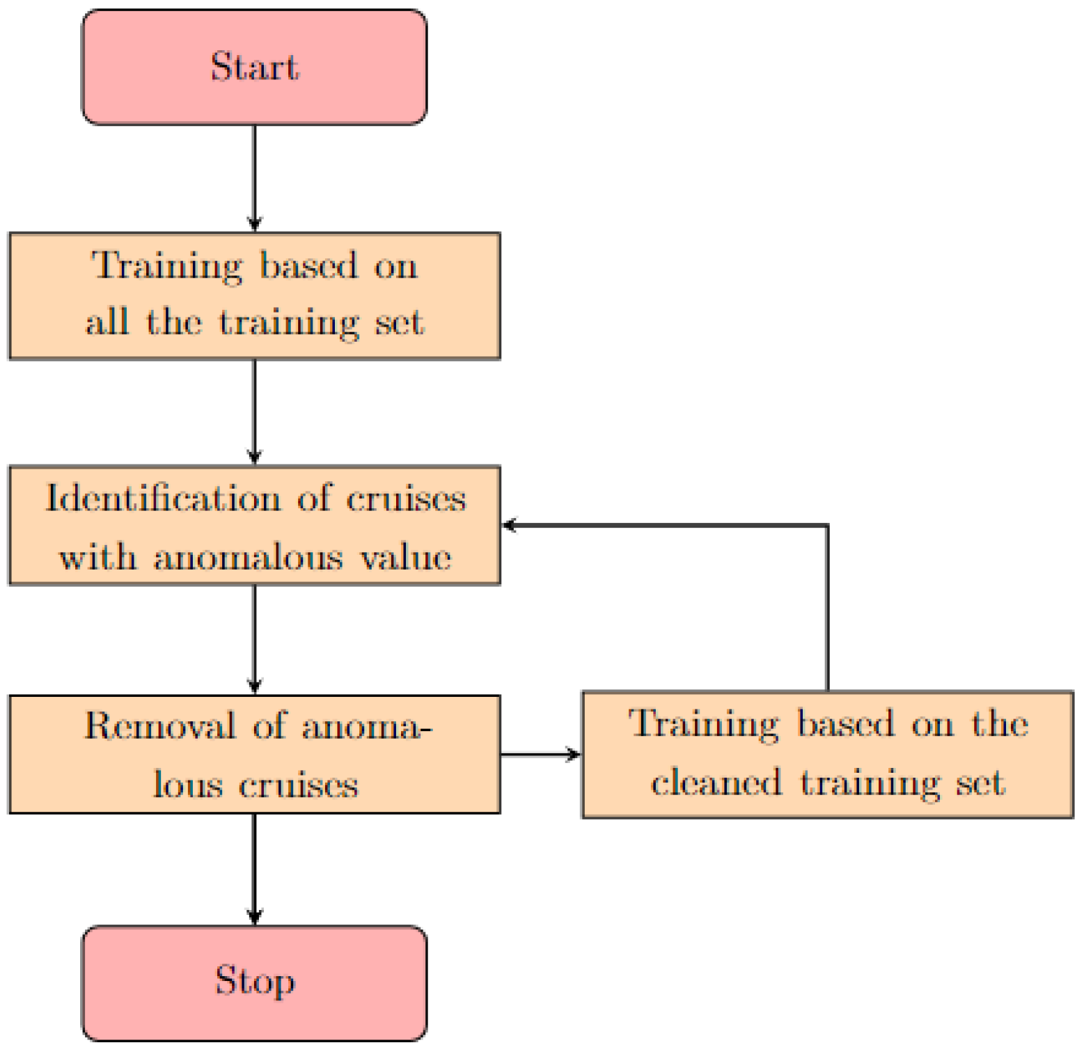
To overcome the potential issue represented by anomalous data, we propose a two-step quality check routine for the removal of incorrect data, which is summarized through the flowchart in Figure 1. First, the model is trained on the whole dataset. Thereafter, the subsets with anomalous data are identified and removed, both from the training and testing set by looking at values that fell inside the $0.1\%$ of the highest error prediction and checking whether they belong to any specific and circumscribable subset (e.g., same sampling cruise, date or provider). The last criterion was applied only if at least the $25\%$ of the samples of the subset were classified as outliers. Subsequently, the model is trained among the cleaned dataset and the process is repeated until no more predictions are cataloged as unreliable.

The final dimensions of the training datasets are reported in

Table 2. Dimension of the training set for each variable, after the removal of noisy and unreliable data.

NO${}_3^{-}$	PO${}_4^{3-}$	Si(OH)${}_4$	A${}_{\mathit{T}}$	Chl-a	NH${}_4$${}^{+}$
$20.686$	$25.335$	$16.187$	$1.292$	$6.040$	$9.900$

.

2.5. Prediction Confidence Interval

Besides providing a prediction, it would be useful to quantify the correspondent uncertainty. This kind of information proves important as we are dealing with values collected over large and not homogeneous areas.

Let us consider, for this task, the so-called confidence interval [26], a quantity widely used in the statistic field, which quantifies the uncertainty of a prediction.

Neural network ensembles, usually referred to as deep ensembles, in addition to being a widely used and successful technique for the improvement of predictive performance, is also a practical and, most importantly, scalable method for predictive uncertainty estimation [27]. See [28] for a more in-depth introduction.

The uncertainty of the model prediction is calculated by providing ten outputs for a given input by changes in the network topologies, such as the number of neurons in each layer. The confidence interval is given by the difference between the third quartile and the first quartile computed over the set containing the 10 different predictions. In fact, the range comprised between these two quantities has been demonstrated to be a solid indicator of the reliability of ensemble deep learning predictions [28].

3. Results

Individual training and testing fitness (both MAE and RMSE) are computed for each of the six variables. Only testing fitness is reported in

Table 3. Comparison of the fitness values (MAE and RMSE) between the current state of the art, Canyon-Med [15], and our method.

		NO${}_3^{-}$	PO${}_4^{3-}$	Si(OH)${}_4$	A${}_{\mathit{T}}$	Chl-a	NH${}_4$${}^{+}$
MAE	Canyon-Med	0.47	0.026	0.40	6.5
MAE	Our method	0.26	0.019	0.31	5.6	0.09	0.13
RMSE	Canyon-Med	0.73	0.045	0.70	11.1
RMSE	Our method	0.50	0.031	0.58	8.2	0.017	0.21

, together with a comparison with results achieved by [15], which represents the current state of the art for the Mediterranean Sea application. The results show a general decrease in both fitness metrics. The largest decreases in the skill metrics (30–45%) are in NO${}_3^{-}$, PO${}_4^{3-}$ and Si(OH)${}_4$, while alkalinity showed the lowest improvements ($15\%$).

Figure 2 compares, via scatter-plot, the real value of the in situ measurements (on the x-axis) with the corresponding prediction of the model (on the y-axis). The nearer a point is to the diagonal, the more the prediction has been performed correctly. The plots confirm that, among the variables, the NO${}_3^{-}$, PO${}_4^{3-}$ and Si(OH)${}_4$ points are fairly well distributed along the diagonal. Chlorophyll-a and NH${}_4^{+}$ points are more scattered. The number of data of A${}_T$ are lower than the other variables, and this might represent a limit in the robustness of the results.

Figure 3 shows, via scatter-plots, the relation between the error obtained by our model (on the x-axis) and the range between the third quantile and first quantile (on the y-axis), which represents the confidence interval. These scatter plots show that a small quantile difference corresponds to small errors in the prediction, confirming the reliability of this metric for computing the confidence interval. The fact that the dispersion of the ensemble predictions is generally low when the errors are low also highlights that predictions are less sensitive to the topology of the network. A few points lie on the bottom-right of the plot, showing low dispersion for poor predictions, which may indicate the presence of outliers not identified by our two-step analysis. Among the variables, NO${}_3^{-}$, PO${}_4^{3-}$, and Si(OH)${}_4$ are those with a larger number of poor predictions with low dispersion.

Figure 4 displays a series of histograms collecting the distribution of the test data as a function of their latitude, longitude, and depth. For each distribution bin, the number of predictions with the $25\%$ ($25\%$ HE) and $10\%$ ($25\%$ HE) highest errors is reported in the darker colors. The figure allows investigation of the presence of inhomogeneity between data distribution and error distribution.

Firstly, histograms of NO${}_3^{-}$, PO${}_4^{3-}$, Si(OH)${}_4$, and chlorophyll-a show good and fairly homogeneous coverage in terms of latitude, while the latitude distribution is biased by the presence of the three major basins in the Mediterranean Sea (western, Adriatic and Levenative basins). Alkalinity shows a biased distribution, with the largest number of observations being gathered in the Northern Adriatic Sea. NH${}_4^{+}$ shows a biased coverage with observations mainly sampled in the Adriatic Sea.

The distribution of $10\%$ HE in the predictions is uniform along the horizontal dimension (both latitude and longitude) for all the variables, except for PO${}_4^{3-}$ and Si(OH)${}_4$. These two variables present a higher frequency of $10\%$ HE for latitudes ranging between 41–42 N. In particular, the percentage of $10\%$ HE prediction in this area are $30\%$ and $20\%$ for PO${}_4^{3-}$ and Si(OH)${}_4$, respectively. On the other hand, the distribution of $10\%$ HE on the depths dimension (third column of the plots) shows that the predictions are more accurate on the surface for all variables and that the percentage of samples characterized by $10\%$ HE increases along the depth. Specifically, the ratio between $10\%$ HE samples and total samples available is about (always above) $20\%$ for depths over 100 m.

These plots can be exploited as further indicators for the reliability of a prediction, e.g., if our model is applied to samples that belong to a geographical area that the model has proven to predict with higher precision, the corresponding result can be labeled as reliable with higher confidence. Conversely, geographical areas showing the presence of $25\%$ HE or $10\%$ HE cases higher than usual should be more carefully investigated given the presence of peculiarities diverging from the mean model.

The diagnostic metrics of Figure 2, Figure 3 and Figure 4 provide an overall picture to assess the level of goodness of the reconstruction for each of the six variables.

Regarding the nitrate, Figure 2a shows that the prediction satisfactorily approximates the observations.

For the phosphate variable (Figure 2b), a similar behavior with respect to the nitrate emerges: the model skillfully predicts both the lower and higher ranges of values.

The prediction of silicate is the one that leads to more satisfactory results, as shown in Figure 2c.

Positive results are also obtained for alkalinity (Figure 2d), even if the bias distribution of the observations (Figure 4) may prevent us from drawing adequate conclusions on error distribution in these zones.

As regards chlorophyll-a (Figure 2e), a clear difference emerges in the quality of prediction for different ranges of values: lower values are predicted more accurately than higher ones. The underlying reason is the gap between the quantity of high- and low-value samples available in the training set.

Finally, taking into account ammonium, Figure 2f shows that this marine variable is the one predicted less accurately. Given that ammonium distribution depends on many interacting and complex biological and chemical processes [29,30], it is not surprising that the explicative variables of our models were not sufficient to reconstruct this variable. Additionally, the biased spatial distribution (e.g., most of the observations gathered in the Adriatic Sea—43–46 N of latitude and 13–18 W of longitude) might not have helped the model’s ability to map ammonium variability in the Mediterranean Sea. Indeed, the largest number of bad predictions accumulated in this marginal sea.

3.1. Prediction of Low Frequency Sampled Variables Starting from Argo Collected Input Data

An important application of the proposed deep learning model is the prediction of nutrient concentrations and carbonate system variables starting from the input provided by the BGC-Argo floats mounting temperature, salinity and oxygen sensors (as mentioned in Section 1), in order to contribute to tackling the undersampling problem between low-frequency and high-frequency observed variables.

Additionally, besides the potential use of our model to provide reliable estimates for non-observed variables, it can be used as a powerful quality check for the observed variables, such as nitrate. In fact, the comparison of our model prediction with BGC-Argo profiles can spot inconsistencies and biases and provide information, if necessary, to adjust the raw data. An example of profiles predicted by our model is shown in Figure 5. We provide as input vectors the time and the geolocation of the BGC-Argo floats together with the profiles of the temperature, salinity, and oxygen density. The plot shows the comparison between the nitrate profile predicted by our model and the two different floats selected for two different areas in the Mediterranean Sea:

• SD6902954: located at $42.89$ N $7.66$ E, with samples for the date 13 June 2019.
• SD6903250: located at $41.85$ N $17.88$ E, with samples to the date 3 December 2019.

As a general comment, the model predictions are fairly good (Figure 5), in the sense that both the typical shape of nitrate profiles and the typical values of nitrate in the deeper layers (i.e., 8 mg m${}^{-3}$ and 4 mg m${}^{-3}$ in SD6902954 and SD6903250, respectively) are very satisfactorily reproduced. A closer inspection of the plots reveals a potential weakness of our model: the reconstruction profiles are not as smooth as would be expected. This is probably a consequence of the fact that the model is trained on punctual data, resulting in unawareness of the typical shape of the profiles of the biogeochemical variables that they try to infer.

Finally, the skill metrics of the reconstructed BGC-Argo nitrate profiles confirm the rather good performance of our model. In fact, the MAE and RMSE computed on about 2200 nitrate profiles for the period 2015–2020 are, respectively: $0.75$ and $0.87$. These values are similar to the ones computed on test set data, demonstrating the quality of the model even with an independent and much bigger dataset.

4. Discussion and Conclusions

This paper investigates a deep learning framework for the prediction of low-frequency sampled variables (such as nutrient concentrations and carbonate systems variables) starting from high-frequency sampled ones (specifically: salinity, and oxygen) and ancillary information such as time and geolocation of the sampling. The method was already proposed [10,11,12,13,14,15], and we applied some improvements specifically for the Mediterranean Sea: a larger training dataset [18], a new two-step quality check routine to improve the dataset and a confidence interval relative to the prediction, exploiting the concept of deep ensembles of neural networks. The method was then accurately validated, and the results show a significant improvement with respect to the state-of-the-art, for all the (fitness) metrics and for all the variables.

The improvement in results over previous applications [15] is due to several factors. First, the dataset used is characterized by a larger amount of samples and wider coverage of the Mediterranean Sea area. Even if this would be not a surprising aspect, it is important to note that given the nature of marine data (i.e., sparse and spatially biased, noisy and potentially with inconsistencies), it was not a given result.

The dataset has been further improved by the two-step quality check routine that leads to the removal of noisy and unreliable samples. During the whole process, our goal was to find an equilibrium between the necessity to delete problematic data and, at the same time, avoid the removal of cruises that lead to important information for the prediction. To ensure the reliability of our method, we randomly checked some samples extracted from cruises that our method rejected. Particular attention, during this process, has been paid to avoid introducing a bias in the spatial distribution of the sample for the different areas of the Mediterranean Sea. This is achieved by stopping the iteration of the check before a bias in the spatial distribution appeared. Our quality check procedure can also be applied to other assembling datasets (or data collection such as Emodnet ones [21]) where multiple sources are merged and possible standardization, conversion and transcription errors can go unnoticed.

Furthermore, the deep learning architecture has been modified (e.g., nonlinear functions between layers, the number of neurons per layer, the optimization algorithm for training, and so on) in order to improve the prediction performance. Finally, thanks to the information stored in the EMODnet dataset, we tested the prediction of two additional variables not previously investigated: chlorophyll-a and ammonium (NH${}_4^{+}$). Results for these variables are satisfactory, allowing us to further the potentiality of our application.

We would also like to underline that we obtained a reduction of the fitness with a faster method, which requires far fewer computational resources compared to the one introduced in [15], which is based on a Bayesian framework. In fact, we observed that training our model with a Bayesian architecture (not shown) instead of the non-Bayesian one did not lead to an improvement in the prediction performance. This is a consequence of the bigger (and quality-checked) dataset used for the training.

This model can prove useful for several reasons. First, a possible application is to infer values of carbonate system variables and nutrients starting from samples collected through BGC-Argo float sensors (when they are equipped with the oxygen sensor). Given the cost of the other biogeochemical sensors [7], this represents a step towards the further exploitation of this observing system. Secondly, model predictions can be used for real-time quality checks of raw variables effectively observed by full-equipped BGC-Argo floats. At present, the quality check of BGC-Argo variables relies on classic statistical procedures [31], while our model prediction can provide a further and easy-to-compute comparison term to spot inconsistencies and biases in these data. This will allow us to have a richer and more detailed knowledge of the Mediterranean Sea basin, which is essential information, especially to understand how the marine environment is changing as a result of the anthropic impact.

In any case, as pointed out in Section 3.1, MLP reconstructions denote the inability in the generation of a smooth and regular curve. In fact, marine variables are not only characterized by specific values of concentration, but also typical shapes of the profiles that inform about ongoing processes and dynamics [32,33]. Thus, the addition of information on the shape of profiles, such as typical patterns in image reconstruction, can be an important element to be added. So, a possible improvement can be to test an approach based on convolutional deep learning architecture [34,35] to reconstruct nutrient profiles from information such as sampling time, geolocation, and profiles of temperature, salinity, and oxygen. Thus, spatial-aware architecture could overcome such issues and lead to the generation of smooth predicted profiles.

The Mediterranean Sea is characterized by significant physical and biogeochemical gradients at different spatial scales [36,37]. The uneven coverage of the data impacted the capability of the network to predict the large range of variability of the variables. Indeed, our results (Figure 4) showed the presence of potential biases linked to local unresolved variability. Therefore, it would be interesting to investigate if introducing a restriction on the investigated areas can provide more precise results. However, while the restriction of the area allows having more data over more homogeneous variability, it can also reduce the number of available data for the training below a safe limit. Our results confirm the previous evidence of [10,14,15], namely that some biogeochemical proprieties can be successfully predicted by neural networks using temperature, salinity, oxygen, and geolocalization. The rationale lies in the fact that the same processes (e.g., transport and biogeochemical processes) concurrently shape the spatial patterns of different variables. The choice of the predictive variables is not the result of an optimization process, but reflects the fact that those variables are the most common and less expensive sensors in the Argo platforms [31,38]. It would be interesting to take the idea further and test the goodness of fit even when only the temperature and salinity are considered. While it is reasonable to expect that prediction power would decrease, the number of available floats would increase at least 5-fold.