Multivariate Transfer Passenger Flow Forecasting with Data Imputation by Joint Deep Learning and Matrix Factorization

Abstract

Accurate forecasting of the future transfer passenger flow from historical data is essential for helping travelers to adjust their trips, optimal resource allocation and alleviating traffic congestion. However, current studies have mainly emphasized predicting traffic parameters for a single type of transport, while lacking research into transfer passenger flow influenced by multiple factors across different transport modes. Additionally, efficient traffic prediction relies on high-quality traffic data, yet data loss issues are inevitable but often ignored. To fill these gaps, we present for the first time a reliable joint long short-term memory with matrix factorization deep learning model (i.e., Joint-IF) for accurate imputation and forecasting of transfer passenger flow between metro and bus. This hybrid Joint-IF model uses a repair-before-prediction strategy to deliver the final high-quality outputs. In particular, we simulate a variety of missing combinations under the natural conditions and apply a low-rank matrix factorization to infer those lost values. In addition, we investigate the effects of crucial parameters and spatiotemporal features on transfer flow prediction. To validate the effectiveness of Joint-IF, a large series of experiments are carried out for models’ comparison and validation on the real-world transfer passenger flow dataset of the Shenzhen public transport system, and the results show that the proposed Joint-IF performs better for both imputation and forecasting of transfer passenger flow relative to the baseline models in terms of accuracy and stability.

1. Introduction

Modern society is facing serious traffic challenges, including traffic accidents, congestion and pollution, and accurate traffic prediction holds the key to alleviating these issues [1]. Normally, traffic forecasting is performed to assess the flow, speed and density of urban road networks, and rarely involves transfer flow between different transport tools. However, due to the constraints of urban network structures and running schedules, some commuters need to transfer between different transport modes to arrive at their final destinations [2]. Usually, commuters in metropolitan areas make reasonable plans before traveling. Especially for remote areas without direct access, effective and less delayed transit transfers can not only greatly enhance commuters’ travel comfort but also help to alleviate urban traffic congestion by dispersing crowds more rapidly. Meanwhile, urban rail transit systems worldwide experienced a rapid expansion in scale and large increase in demand before the pandemic [3]. A future trend of urban transport progress is building comprehensive traffic systems with metros as the backbone and public transport as a form of assistance in the post-pandemic era [4]. Hence, determining how to conduct mathematical modelling and algorithm analysis on the collected historical transfer passenger flows of different modes of transport to establish a high-performance forecasting model, and finally estimate future transfer passenger flow, is crucial. Accordingly, transport operators should develop Sustainable Mobility as a Service (S-MaaS) solutions [5,6] that integrate different forms of transportation and services, with their supply components ultimately providing more effective transfer services for public transport.

In urban transportation systems, metro and bus, two of the most convenient transport services, dominate public transportation. As of late 2019, China had 40 cities with rail transit, or metro as a narrow definition [4], and this trend is accelerating. Hence, there are a large amount of transfer services between buses and metro stations that are suitable as a target of our research. In this era of big data, a large number of traffic data forecasting techniques have been proposed. Concretely, the available traffic forecasting algorithms can be roughly divided into classical and machine learning (ML) methods, the former of which can be further subdivided into traditional linear methods and statistical learning methods. To be more specific, earlier research efforts focused on historical averages [4,7], smoothing techniques [7,8] and later autoregressive integrated moving averages (ARIMA) [9] and its variants. Moreover, the decomposition-based statistical learning approaches, specified as matrix factorization, can accomplish the forecasting and even imputation tasks through a low-rank matrix factorization (LRMF) capturing spatial–temporal dependencies [10]. Nevertheless, the overly strict assumptions required by these methods have hindered the utilization of large-scale traffic data modelling processes [8,11]. Currently, studies on predicting traffic value using the popular ML-based methods have made significant progress compared with non-ML models [12], such as support vector machine (SVM), decision tree (DT), extreme gradient boosting (XGBoost) and random forest (RF), which are frequently utilized for traffic prediction tasks due to their superior abilities to capture partial complex spatiotemporal correlations from small incomplete datasets. In fact, it has been proven that deep learning (DL) is an emerging technology due to its good fitting capability [13]. As a hot research topic, several existing DL models perform well in traffic prediction, including long short-term memory (LSTM) and convolutional-based neural networks [1]. In particular, LSTM, a variant of recurrent neural networks (RNN), is capable of alleviating the vanishing gradient and effectively tackling the network-level time series forecasting problem [13].

Nevertheless, we still face great challenges. One of the key methodological challenges of traffic data fusion application is to integrate multi-source (i.e., metro and bus passenger flow) observations, while the existing studies only perform single-source data forecasting. Next, because of the variable factors influencing transfer demand, current traffic prediction methods are not capable of completing the forecasting tasks for multi-variate transfer passenger flow, especially for incomplete traffic datasets caused by various hardware/software failures (e.g., equipment errors, communication troubles or bad weather). Like other time series, transfer passenger flow usually contains both linear and non-linear spatiotemporal modes, and the expected transfer model must be able to solve the problem of extreme flow, as passengers always arrive at short notice. To fill the gaps and tackle such concerns in existing studies, a joint DL-based model with MF imputation is created and tested for multivariate transfer passenger flow forecasting in this study.

Correspondingly, the main contributions of this paper are as follows:

• We provide a reliable multivariate prediction model of Joint-IF by taking into account a variety of spatiotemporal factors (e.g., weather and location) for the accurate and efficient calculation of transfer passenger flow between metro and bus stations;
• Before performing the multi-interval forecasting task, we adopt an efficient temporal regularized MF for recovering transfer passenger flow under both missing situations to further enhance the robustness of the network-wide forecasting model;
• We conduct a large number of experiments on real-world transfer passenger flow. Compared with the baseline models, the results demonstrate that the proposed Joint-IF predicts the transfer passenger flow with lower error and better robustness.

The rest of this paper is organized as follows. Section 2 briefly reviews relevant work on traffic data modeling. In Section 3, the methodology of transfer passenger flow modeling is described in detail. Section 4 reports extensive numerical experiments and analyzes the performance of Joint-IF. Finally, the concluding remarks are given in Section 5.

2. Related Work

A variety of issues in public transport, such as transfer service [14], still lack in-depth investigation, meaning that few studies have analyzed and forecasted transfer passenger flow among different transport tools. Recently, varied studies on the prediction of the flow, speed and density of single-traffic vehicles have achieved great success [4,9], which are helpful for transfer passenger flow prediction. Herein, we recall the related applications of various forecast techniques on traffic time series, including traffic data imputation and forecasting.

Restricted by the backwardness of data processing, early parametric prediction models (e.g., historical average [7] and Kalman filter [3]) can forecast stable traffic flow well, but fail to deal with the increasing amount of unsteady and non-linear traffic data [15]. Because of this, the availability of traffic data has provided more opportunities for forecasting efforts, and a wide variety of statistical learning methods, including principal component analysis (PCA)-based [11] and decomposition-based [9] algorithms, have been adopted to model traffic data. For example, Xing et al. [16] proposed a robust PCA (RPCA) model for traffic data prediction. Gong et al. [17] introduced three online non-negative matrix factorization (ONMF) methods for traffic crowd flow forecasting. Additionally, it is well known that high-quality traffic data offers a guarantee for highly accurate prediction results [10], and some scholars have studied spatiotemporal data assuming a lack of data entries. Qu et al. [18] put forward a probabilistic PCA (PPCA)-based model to repair missing traffic values. Jia et al. [19] created an imputation model (CIM) for missing traffic congestion data using joint MF. Further, Li et al. [10] introduced a compensated residual MF with spatial–temporal regularization (ST-CRMF) for traffic time series repair and multi-interval forecasting. Moreover, Chen et al. [11] established a Bayesian temporal factorization (BTF) framework for both missing traffic data imputation and multi-step rolling prediction tasks.

Except for the aforementioned approaches, ML and its subclass DL have aroused great academic and industrial interest in the past decades [20]. Of these, traditional ML prediction models, such as SVM, RF, XGBoost [21], wavelet transform (WT) [22] and Bayesian networks [23], have achieved favorable forecasting performance in intelligent transportation systems (ITS). For example, Feng et al. [24] presented an adaptive multi-kernel SVM (AMSVM) with spatiotemporal correlation for short-term traffic flow prediction. After acquiring point-of-interest (POI) data around bus stops, Lv et al. [25] employed an XGBoost to forecast the passenger flows of each bus line. In addition, due to the complexity of ITS, it is difficult for a single ML model to output reliable prediction results, and the hybrid methods connecting multiple algorithms enable the uncertainty and nonlinear characteristics of traffic data to be handled more effectively. Sun et al. [7] built a hybrid Wavelet–SVM model for short-time passenger flow forecasting in Beijing metro. Wen et al. [9] introduced a time-series-decomposition-based forecasting model with transfer learning for rail short-term passenger flow in holiday periods. Complying with further technological innovations, studies on traffic prediction with DL, such as using LSTM-based models to exploit the spatiotemporal properties of traffic data, have clearly outperformed the traditional methods. In fact, LSTM can capture and preserve the long- and short-term nonlinear traffic dynamics in an effective manner, and thus it is widely adopted in transportation fields. Ma et al. [26] first introduced an LSTM network for short-term travel speed prediction. To promote prediction accuracy, Zhao et al. [27] further constructed a cascaded LSTM network considering spatiotemporal correlation for short-term traffic prediction. While solving the traffic forecasting tasks, the revised LSTM-M proposed by Tian et al. [28] also worked for missing traffic value recovery. With these in-depth studies on DL, forecasting models combining LSTM with other DL algorithms (e.g., attentional mechanism, convolutional network and generative adversarial network) were proposed. Zheng et al. [29] presented an attention-based conv-LSTM network to provide more satisfying forecasting accuracy. Furthermore, Khaled et al. [30] suggested an adversarial multi-graph convolutional neural network to capture the global–local dynamic spatial–temporal properties across various nodes at different timesteps for traffic forecasting tasks. As rewarded for ITS, in the desired S-MaaS system, the predicted traffic volumes will provide the optimal solutions for the selection of the supply components [31], such as proactively adjusting the schedules across diverse traffic vehicles and stations, and ultimately improve the efficiency and effectiveness of transport systems [32,33].

Though progress has been achieved in single traffic object forecasting, no study on the transfer flow prediction between different traffic tools has yet been performed. To the best of our knowledge, this is the first study that uses a DL model to perform high-precision forecasting of transfer passenger flow between the most representative transport tools (i.e., metro and bus). Moreover, the final Joint-IF model will also provide a basis for urban public transportation system operation efficiency improvement, people-oriented policy formulation and ITS-based transportation service optimization.

3. Methodology

3.1. Preliminaries

In this work, we concentrate on the tasks of data imputation and prediction based on transfer passenger flow derived from all metro lines and their corresponding bus stops in the Shenzhen public transportation system. Firstly, we define our study objects below.

Definition 1.

Transfer Passenger Flow. Unlike the typical modeling studies on traffic data obtained from single types of vehicles, our study involves transfer passenger flow across metro and bus systems. Specifically, we collected smartcard data recorded on the automatic fare collection system of public transport when passengers transfer between the metro and bus systems, and then organized them as a 2D matrix. Of particular interest is that a metro station might have multiple bus stops; the flows refer to the total number of people from the metro to all its corresponding bus stops, so the flows cannot exceed the number of total exits from the metro. Therefore, taking the metro stations as the horizontal axis, we assume the transfer flow is $\mathit{Y}\in {ℝ}^{M\times N}$, where ${𝓎}_t\in {ℝ}^N$is an observed vector of $N$stations at $t$time steps;$M$is the total number of time slices and ${𝓎}_{i,t}$ is the transfer flow of the $ith$station on the$tth$time point.

Definition 2.

Transfer Flow Imputation. Data loss is difficult to avoid due to various failures, manifested as a certain rate of zeros in matrix $\mathit{Y}=\left\{{𝓎}_1,{𝓎}_2,\cdots ,{𝓎}_t\right\}$. Before starting the prediction task, our repair process works by fitting a high-precision mapping function ${\mathcal{F}}_I\left({\theta }_I\right)$with a partially observed flow, then reconstructing a complete traffic matrix${\mathit{Y}}_{\mathit{I}}$.

Definition 3.

Transfer Flow Prediction. Traffic prediction is a classic time series modeling issue, which takes a series of historical data as input and optimizes a desired model by continuously evaluating and reducing the errors between the true and predicted values in the hope of eventually accurately predicting future traffic data [10]. In this study, given the imputed transfer passenger flow${\mathit{Y}}_{\mathit{I}}$of all metro–bus stations at the previous$H$time slots of its traffic network, our goal is to learn the complex function of ${\mathcal{F}}_F\left({\theta }_F\right)$ in Equation. (1) and then calculate future transfer flow through this mapping relationship:

$$({\widehat{𝓎}}_t\mathbf{,}\cdots \mathbf{,}{\widehat{𝓎}}_{H+2},{\widehat{𝓎}}_{H+1})={\mathcal{F}}_F\left(\left({𝓎}_t\mathbf{,}\cdots \mathbf{,}{𝓎}_{H+2}\mathbf{,}{𝓎}_{H+1}\right)|\left({𝓎}_H\mathbf{,}\cdots \mathbf{,}{𝓎}_2\mathbf{,}{𝓎}_1\right)\mathbf{;}{\theta }_F\right)$$

(1)

where  $\mathcal{F}\left(·\right)$denotes the desired model and $\theta ={\theta }_I\cup {\theta }_F$stands for the learnable parameters.

3.2. Model Architecture

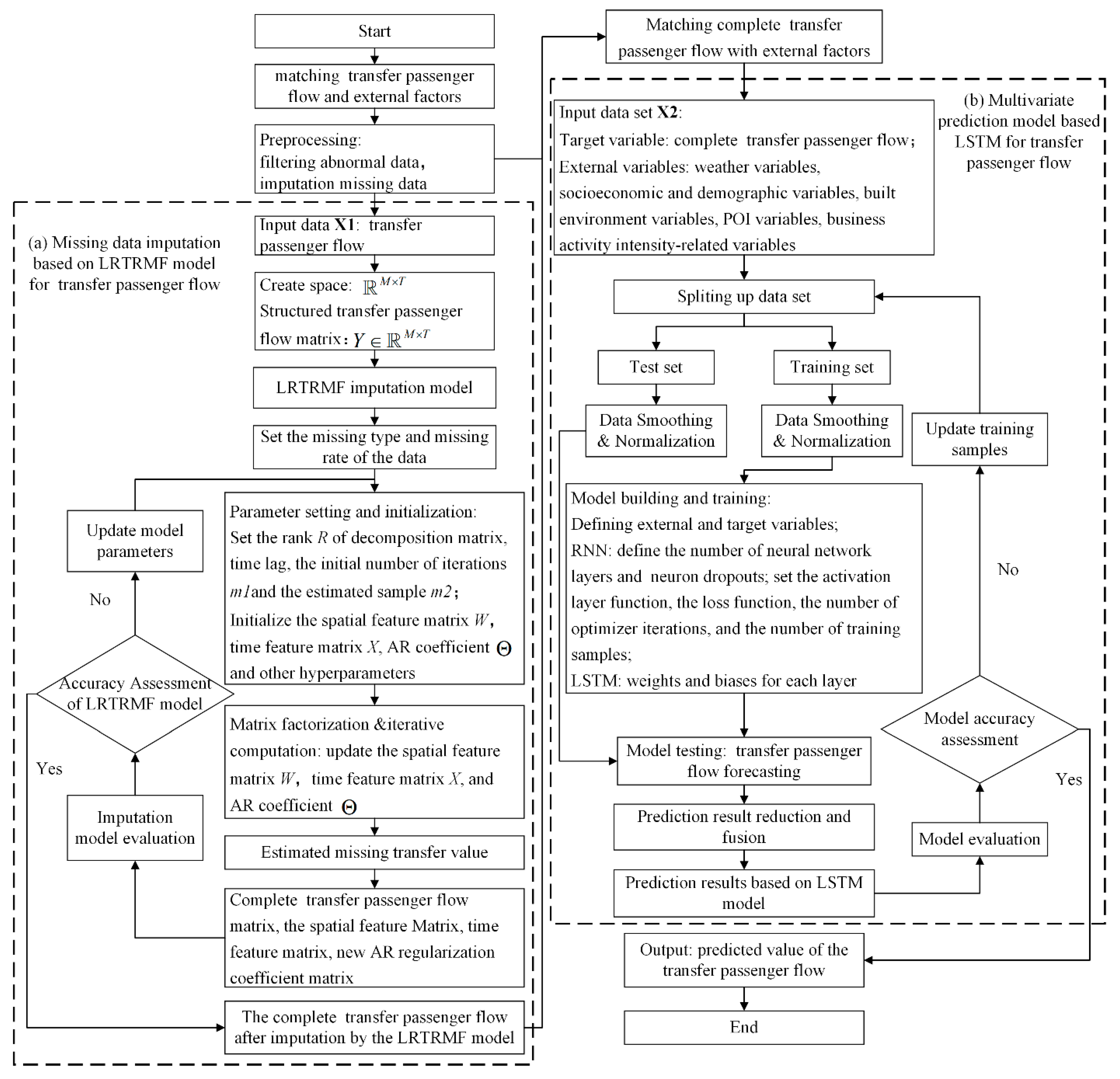
In this section, we propose a novel Joint-IF model to recover and forecast the transfer passenger flow across bus and metro. As shown in Figure 1, the imputation and prediction framework consists of two components: the data preprocessing module (i.e., multi-source data fusion/missing data repair) and LSTM-based multivariate transfer prediction module. Proceeding along the flowchart in Figure 1, we have fulfilled the construction, testing and discussion of the Joint-IF model.

Figure 1. Flowchart of the Joint-IF imputation and forecasting framework.

3.2.1. Matrix Factorization-Based Imputation Module

In our study, the collected original dataset involves transfer flow, weather data, socioeconomic and demographic data, built environment data, business activity intensity data and POI data. In this case, the first variable is the target variable and the others are external factors. Before performing our prediction task, missing data repair is desirable due to the data loss that inevitably occurs during data collection, especially in extreme environments. In general, traditional repair techniques fail to effectively impute missing traffic value [34,35], and so we introduced an LRMF model to fix incomplete transfer passenger flow in the study. In Figure 1, we show the procedure of the LRMF model, and its repair theory can be described as follows:

Given the transfer passenger flow $\mathit{Y}\in {ℝ}^{M\times N}$, it can be decomposed into a spatial factor matrix $\mathit{W}\in {ℝ}^{R\times M}$ and a temporal factor matrix $\mathit{X}\in {ℝ}^{R\times N}$. The standard MF is below:

$$\mathit{Y}={\mathit{W}}^T\mathit{X}$$

(2)

The elementwise of MF satisfies the following Equation (3):

$${𝓎}_{i,t}={\mathit{w}}_i^T{\mathit{x}}_t+{\epsilon }_{i,t}$$

(3)

where ${\mathit{w}}_i$ is the $i$-th column vector of the spatial matrix $\mathit{W}$; ${\mathit{x}}_t$ is the $t$-th column vector of the temporal matrix $\mathit{X}$ and ${\epsilon }_{i,t}$ represents the zero-mean noise.

Although the above MF can fix missing/abnormal elements in the matrix using approximate decomposition and reconstruction, it cannot capture the time dependence between different columns in temporal factor matrix $\mathit{X}$. As such, we apply the autoregressive regularizer [36] to deal with the time dependence in $\mathit{X}$, and the formula is as follows:

$${\mathit{x}}_{t+1}={{\displaystyle \sum }}_{k=1}^d{\mathit{\beta }}_k{\displaystyle ⨂}{\mathit{x}}_{t+1-u_k}+{\mathit{\eta }}_t$$

(4)

where $\Pi =\left\{u_1,\dots ,u_k,\dots ,u_d\right\}$ is the time lag; d is the order from the autoregressive model; ${\mathit{\beta }}_k$ denotes a $R\times 1$ coefficient vector; $⨂$ refers to the Hadamard (element-wise) product and ${\mathit{\eta }}_t$ means the Gaussian noise term. Based on Equation (4), the sequence at the next moment can be estimated from the potential temporal matrix X to forecast the ${\widehat{\mathit{x}}}_{t+1}$at the next moment. Additionally, further, given the target variable Y and the MF with training parameters, the general optimization problem can be summarized as Equation (5):

$$\underset{ {\mathit{W}}^{\ast },{\mathit{X}}^{\ast }}{\min }\frac{1}{2}{\displaystyle \sum }_{\left(i,t\right)\in \mathsf{\Phi }}{\left({𝓎}_{i,t}-{\mathit{W}}_i^T{\mathit{X}}_t\right)}^2+\frac{{\lambda }_{\mathit{𝓌}}\eta }{2}\Vert \mathit{W}{\Vert }_F^2+\frac{{\lambda }_{\mathit{𝓍}}\eta }{2}\Vert \mathit{X}{\Vert }_F^2$$

(5)

where $\mathsf{\Phi }$ refers to the set of ($i,t$) pairs of the matrix elements; the factors $\Vert \mathit{W}{\Vert }_F^2$ and $\Vert \mathit{X}{\Vert }_F^2$ are applied for overfitting prevention and stability enhancement, and their coefficients ${\lambda }_{𝓌}$, ${\lambda }_{𝓍}$ and $\eta$ control the degree of normalization. By continuously solving the reverse gradient approximation, we can acquire the efficient matrices $\mathit{W}$ and $\mathit{X}$, then approximate the elements in $\mathit{Y}$ using ${\widehat{𝓎}}_{i,t}\approx {\mathit{w}}_i^T{\widehat{\mathit{x}}}_t$ and eventually repair missing traffic value in $\mathit{Y}$. In fact, our imputation module provides a scalable and flexible scheme to augment the quality of multivariate transfer passenger flow to facilitate the subsequent forecasting task.

3.2.2. Deep-Learning-Based Forecasting Module

The further purpose of this section is to provide accurate information on transfer passenger flow. Referring to the related literature, we find that transfer passenger flow is influenced by several factors in time and space and thus we consider their effects on transfer passenger flow in our forecasting model. As is known, LSTM is an excellent variant [37] of the RNN algorithm which is capable of learning the long-term dependencies of time series data well so that it exhibits excellent performance in traffic data forecasting tasks. Hence, we applied the LSTM to accurately predict transfer passenger flow after considering multiple feature variables.

The key for LSTM to effectively tackle the gradient vanishing and gradient explosion problems of RNN lies in its designed gating structures, i.e., input, output and forget gates. Of these, given in Equation (6), the main function of the forget gate ${\mathit{f}}_t$ is to decide which information should be discarded or reserved. Specifically, the information from the previous hidden state (${\mathit{C}}_{t-1},{\mathit{h}}_{t-1}$) and the current input ${\mathit{x}}_{t }$ is passed into the sigmoid function concurrently. Additionally, the output ${\mathit{f}}_t$ is between 0 and 1, with a value closer to 0 meaning it should be discarded and a value closer to 1 meaning it should be retained:

$${\mathit{f}}_t={\mathsf{\delta }}_{\mathrm{sigmoid}}\left({\mathit{\omega }}_g·\left[{\mathit{h}}_{t-1},{\mathit{x}}_t\right]+{\mathit{b}}_g\right)$$

(6)

where ${\mathit{\omega }}_g$ and ${\mathit{b}}_g$ represent the weight and bias of the forget gate, respectively; $\delta$ is an activation function and $\left[{\mathit{h}}_{t-1},{\mathit{x}}_t\right]$ is the new vector obtained by merging the vector ${\mathit{h}}_{t-1}$ and ${\mathit{x}}_t$.

As shown in Equation (7), the input gate${\mathit{i}}_{t }$is used for updating the cell state. In particular, the sigmoid function receives this information from the previously hidden layer ${\mathit{h}}_{t-1}$ and the current input ${\mathit{x}}_t$, and then outputs a value between 0 and 1 to determine which information to update, where 0 denotes that the information is not important and 1 signifies importance. Additionally, in Equation (7), the above information is also passed into the tanh function to create a new candidate vector ${\tilde{C}}_t$, whose output is multiplied by the result of the sigmoid function and the output ${\mathit{i}}_t$ from the sigmoid function determines which information needs to be preserved in the output ${\tilde{C}}_t$ of the tanh function.

$${\mathit{i}}_t={\mathsf{\delta }}_{\mathrm{sigmoid}}\left({\mathit{\omega }}_i·\left[{\mathit{h}}_{t-1},{\mathit{x}}_t\right]+{\mathit{b}}_i\right)$$

(7)

$${\tilde{\mathit{C}}}_t={\mathsf{\delta }}_{\tan \mathrm{h}}\left({\mathit{\omega }}_c·\left[{\mathit{h}}_{t-1},{\mathit{x}}_t\right]+{\mathit{b}}_c\right)$$

(8)

where ${\mathit{\omega }}_i$ and${\mathit{b}}_i$ represent the weight and bias of the input gate, respectively, when the activation function is sigmoid;${\mathit{\omega }}_c$ and${\mathit{b}}_c$ are the weight and bias of the input gate when the activation function is tanh.

Later, the previous cell state ${\mathit{C}}_{t-1}$ is multiplied point-by-point with the forget vector ${\mathit{f}}_t$. If it is multiplied by a value close to 0, this means that the information is to be discarded in the new cell state ${\mathit{C}}_t$. Further, this value is added point-by-point with the output value ${\mathit{i}}_t$ of the input gate to update the new information found by a neural network to ${\tilde{\mathit{C}}}_t$. Thus, the updated cell state ${\mathit{C}}_t$ is obtained.

$${\mathit{C}}_t={\mathit{f}}_t⨂{\mathit{C}}_{t-1}+{\mathit{i}}_t⨂{\tilde{\mathit{C}}}_t$$

(9)

Since it contains the information of the previous input, the output gate is utilized to determine the next hidden state. First, the sigmoid function processes the previous hidden state ${\mathit{h}}_{t-1}$ and the current input ${\mathit{x}}_t$, and the new cell state ${\mathit{C}}_t$ is then fed to the tanh function. Last, the output of the tanh is multiplied by the output ${\mathit{o}}_t$ of the sigmoid function to determine the information that the hidden state ${\mathit{h}}_t$ should carry. Further, the hidden state ${\mathit{h}}_t$ is then taken as the output of the current cell ${\mathit{C}}_t$, and the cell state ${\mathit{C}}_t$ and the hidden state ${\mathit{h}}_t$ are passed to the next time step.

$${\mathit{o}}_t=\mathrm{sigmoid}\left({\mathit{\omega }}_o·\left[{\mathit{h}}_{t-1},{\mathit{x}}_t\right]+{\mathit{b}}_o\right)$$

(10)

$${\mathit{h}}_t={\mathit{o}}_t⨂\tan \mathrm{h}\left({\mathit{C}}_t\right)$$

(11)

3.3. Algorithm Complexity Analysis

In this section, we will further analyze the complexity of the proposed Joint-IF, which mainly consists of time complexity and space complexity. Concretely, the time complexity of the Joint-IF denotes the time consumed to complete the imputation and prediction tasks. Additionally, the additional space complexity indicates the space required to achieve the same task mentioned above, which is measured by the size of the space in which all data are stored. All in all, the complexity of Joint-IF can be denoted as a function whose domain is the size of the input values, and its range of values usually takes the number of steps to be executed (time complexity) or the storage space required (space complexity). In our study, the synthesis ability of Joint-IF relies on the premise that time and space resources reach a balance.

Time Complexity: the time complexity of Joint-IF is expressed as$\mathrm{o}\left(n_M\ast n_N+nb\right)$, in which $b$ is the number of parameters and $n$ represents the number of samples. During the missing data imputation stage, the time complexity depends on the dimension of the input matrix $\mathit{Y}$, i.e., its time complexity is $\mathrm{o}\left(n_M\ast n_N\right)$. In the prediction stage, the time complexity relies on the number of feature variables and the number of samples, i.e., its time complexity is $\mathrm{o}\left(nb\right)$. Therefore, the total time complexity of Joint-IF is the $\mathrm{o}\left(n_M\ast n_N+2nb\right)\approx \mathrm{o}\left(n_M\ast n_N\right)\approx \mathrm{o}\left(n^2\right)$, where $n$ is much larger than $m$.

Space Complexity: the space complexity of Joint-IF is the$\mathrm{o}\left(n^2+z^{2}k\right)$, where$k$is the number of neural network layers and $z$ represents the number of neurons per layer. In the missing data recovery stage, the space complexity depends on the maximum space (the data size) required for data storage, i.e., its space complexity is $\mathrm{o}\left(n^2\right)$. During the forecasting stage, the space complexity of Joint-IF relies on the number of layers and the number of neurons, i.e., its space complexity is $\mathrm{o}\left(z^{2}k\right)$). Thus, the total space complexity is the $\mathrm{o}\left(n^2+2z^{2}k\right)\approx \mathrm{o}\left(n^2\right)$, where $n$ is much larger than $z$, $k$.

3.4. Model Implementation

In summary, the proposed Joint-IF model mainly consists of an LRMF-based missing data imputation module and an LSTM-based multivariate prediction module for transfer passenger flow. The pseudo-code of this Joint-IF is described in Algorithm 1 below.

Algorithm 1: Training Procedure of the Joint-IF Model

Input: Feature vectors q; transfer passenger flow matrix $\mathit{Y}\in {ℝ}^{M\times N}$; rank R; missing rate and missing scenarios; $\Pi =\left\{u_1,\dots ,u_k,\dots ,u_d\right\}$ as the time lag; a spatial matrix $\mathit{W}\in {ℝ}^{R\times M}$ and a temporal matrix $\mathit{X}\in {ℝ}^{R\times N}$; AR regularized coefficient matrix $\Theta$; the number of initial iterations $m_1$ and the number of estimated samples $m_2$.

Output: Forecasting results $\widehat{\mathit{Y}}$ of the transfer passenger flow

Initialization: Training parameters of the Joint-IF framework

Begin

For $i$ to $m_1$ + $m_2$ do

Calculate and update the spatial matrix $\mathit{W}$:

${\mathit{w}}_i={\left(\sum _{t:\left(i,t\right)\in \Omega }{\mathit{x}}_t{\mathit{x}}_t^T\right)}^{-1}\sum _{t:\left(i,t\right)\in \Omega }{\mathit{y}}_{i,t}{\mathit{x}}_t$

Calculate and update the temporal matrix X:

For $t$ = 1, 2, …, $m_1$, update X:

${\mathit{x}}_t={\left(\sum _{i:\left(i,t\right)}{\mathit{w}}_i{\mathit{w}}_i^T+{\lambda }_x\eta I\right)}^{-1}\sum _{i:\left(i,t\right)\in \Omega }{\mathit{y}}_{i,t}{\mathit{w}}_i$

For $t$ = $m_1$ + 1, 2, …,$m_1+m_2$, update X:

${\mathit{x}}_t={\left({\displaystyle {\displaystyle \sum }_{i:\left(i,t\right)\in \Omega }}{\mathit{w}}_i{\mathit{w}}_i^T+{\lambda }_{x}I+{\lambda }_x{\displaystyle {\displaystyle \sum }_{h\in \Pi ,t+h\le N}}\mathrm{diag}\left({\mathit{\theta }}_h⨂{\mathit{\theta }}_h\right)+{\lambda }_x\eta I\right)}^{-1}\left({\displaystyle {\displaystyle \sum }_{i:\left(i,t\right)\in \Omega }}{\mathit{y}}_{i,t}{\mathit{w}}_i+{\lambda }_x{\displaystyle {\displaystyle \sum }_{u\in \Pi }}{\mathit{\theta }}_u⨂{\mathit{x}}_{t-u}+{\lambda }_x{\displaystyle {\displaystyle \sum }_{u\in \Pi ,t+u\le N}}{\mathit{\theta }}_h⨂{\mathit{\psi }}_{t+h}\right)$

Calculate and update the AR coefficients $\mathit{\Theta }$:

${\theta }_h={\left({\sum }_{t=m_1+1}^{m_1+m_2}\mathrm{diag}\left({\mathit{x}}_{t-h}⨂{\mathit{x}}_{t-h}\right)+\frac{{\lambda }_{\theta }}{{\lambda }_x}I\right)}^{-1}\left({\sum }_{t=m_1+1}^{m_1+m_2}{\mathit{\pi }}_t^h⨂{\mathit{x}}_{t-h}\right)$

Recover missing values in $\mathit{Y}$ and update it.

Return complete transfer passenger flow $\tilde{\mathit{Y}}$.

Matching target variable $\tilde{\mathit{Y}}$ and feature vectors q as the input of the prediction module.

For $i$ to $m_1$ + $m_2$ do

Forecasting future transfer passenger flow $\left\{{𝓎}_{t+T}^{*},{𝓎}_{t+T-1}^{*},\dots ,{𝓎}_{t+2}^{*},{𝓎}_{t+1}^{*}\right\}$ by Equations (6)–(11).

End for

Return $\widehat{\mathit{Y}}$ as the prediction results of transfer passenger flow.

4. Numerical Experiments

We conducted extensive experiments on a real-world dataset to evaluate the Joint-IF model and finally complete the task of predicting transfer passenger flow with missing values.

4.1. Dataset Description

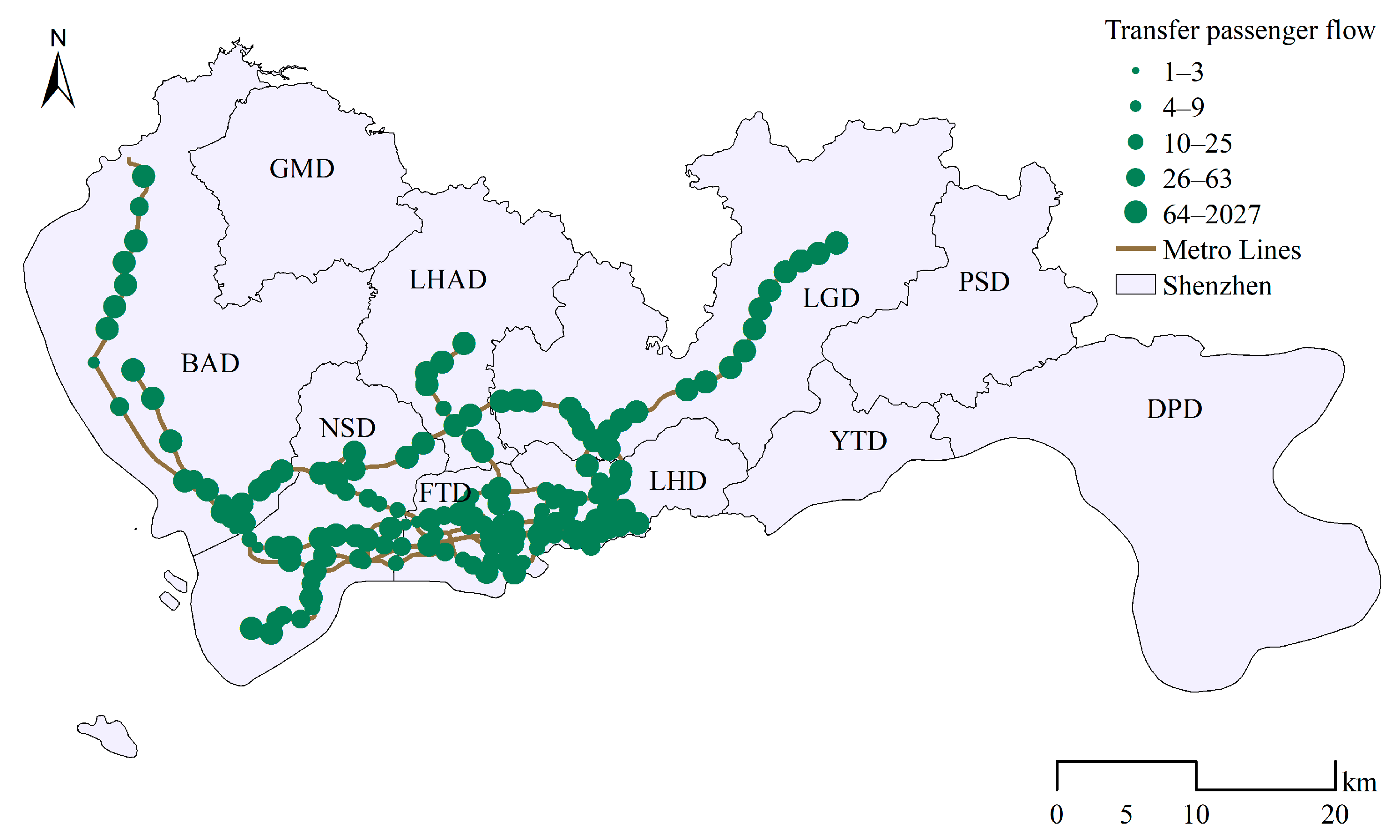
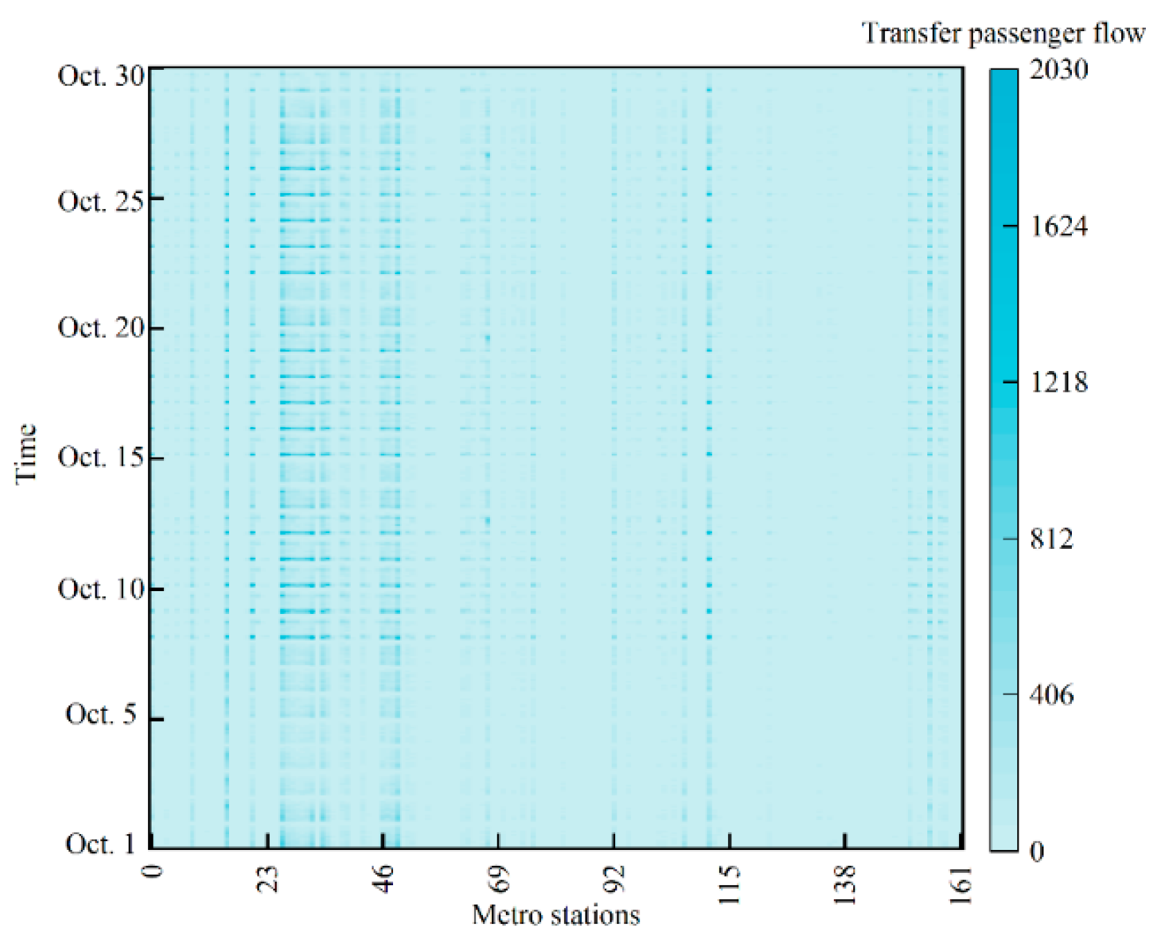
To train Joint-IF and compare its performance with several advanced models, we selected the transfer passenger flow between metro and bus and other external factors in Shenzhen’s public transportation transaction system [38] as the dataset. Herein, the whole data collection procedure lasted for 30 days from 1 October to 30 October in 2017 at hourly intervals. Figure 2 depicts the spatial distribution of metro lines, metro stations and transfer passenger flow. Figure 3 shows the distribution of transfer passenger flow at all metro stations.

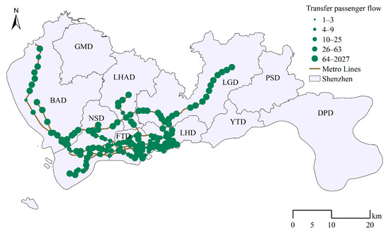
Figure 2. Spatial distribution of the study areas and transfer passenger flow therein.

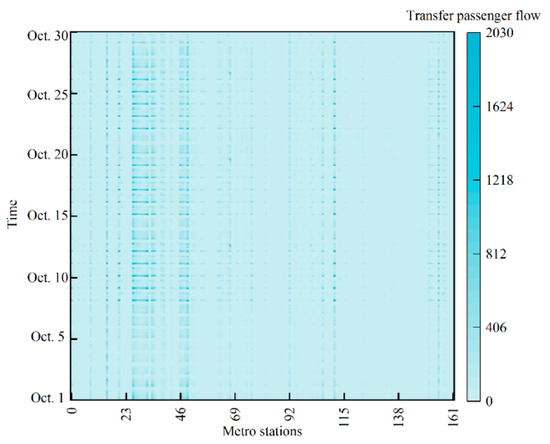
Figure 3. Distribution characteristics of the transfer passenger flow at all metro stations.

Similarly, the external factors have significant influences on transfer flows, including weather variables (e.g., wind speed, temperature, visibility and rainfall), socio-economic level, demographic variables (e.g., housing price, rent, GDP near metro site and population density), built environment variables (e.g., the transfer distance between metro and bus lines, the number of bus lines and their stops near metro sites and the distance between metro distance from CBD), and POI information (e.g., the scenic spots, business housing, technology, culture, finance, insurance, shopping mall and accommodation services near a metro station). Notably, these external factors require reformatting to better match transfer flow, and they are integrated and fed into the prediction model but without being predicted. Table 1 outlines the definitions and statistical properties of all the target and external variables.

Table 1. Definition and statistical characteristics of the target and external variables.

Variables		Definitions	Unit	Mean	Sd.
Target variable	Transfer passenger flow	The number of transfer passengers per hour at each metro station	Persons	56	131
External factors	Weather variables
	Wind Speed	The maximum wind speed per hour	m/s	3.14	1.34
	Temperature	The maximum temperature per hour	°C	26.74	3.47
	Visibility	Minimum visibility per hour	m	33.75	10.13
	Precipitation	The cumulative precipitation per hour	mm	0.15	0.93
	Socio-economic and demographic variables (near metro station)
	Housing Price	Average housing prices	$\mathrm{USD}/{\mathrm{m}}^2$	8932.7	2585.9
	Housing Rent	Average housing rent	$\mathrm{USD}/{\mathrm{m}}^2$	12.57	3.26
	Geographical GDP	GDP level	USD billion	40.84	6.71
	Population Density	Hourly crowd density	-	5.62	1.19
	Built environment variables (near metro station)
	Transfer Distance	Average transfer distance between metro station and bus stops	m	328.20	91.65
	Bus Lines	The number of bus lines		19	8
	Bus Stops	The number of bus stops	-	26	11
	Distance from CBD	Distance of metro station from CBD	m	9600	6604
	POI information (near metro station)
	Scenic Spots	Number of scenic spots	-	13	9
	Shopping Malls	The number of shopping malls	-	27	20
	Technology and Culture	The number of technology and culture	-	195	119
	Finance and Insurance	The number of finance and insurance	-	124	123
	Business Housing	The number of business housing	-	214	143
	Hotel Services	The number of hotel services	-	94	88

4.2. Performance Metrics

We adopted four evaluation metrics (i.e., mean absolute percentage error (MAPE), root mean squared error (RMSE), mean absolute error (MAE) and goodness of fit (${\mathrm{R}}^2$)) [39,40,41] to assess and compare the outputs of all models. The detailed formulations of the four indexes are written as follows:

$$\mathrm{MAPE}=\frac{1}{\left|\Omega \right|}{\displaystyle \sum }_{\left(i,t\right)\in \Omega }\left|\frac{{𝓎}_{i,t}-{\widetilde{𝓎}}_{i,t}/{\widehat{𝓎}}_{i,t}}{{𝓎}_{i,t}}\right|\times 100$$

(12)

$$\mathrm{RMSE}=\sqrt{\frac{1}{\left|\Omega \right|}{\displaystyle \sum }_{\left(i,t\right)\in \Omega }{\left({𝓎}_{i,t}-{\widetilde{𝓎}}_{i,t}/{\widehat{𝓎}}_{i,t}\right)}^2}$$

(13)

$$\mathrm{MAE}=\frac{1}{\left|\Omega \right|}{\displaystyle \sum }_{\left(i,t\right)\in \Omega }\left|{𝓎}_{i,t}-{\widetilde{𝓎}}_{i,t}/{\widehat{𝓎}}_{i,t}\right|$$

(14)

$${\mathrm{R}}^2=\frac{{{\displaystyle \sum }}_{\left(i,t\right)\in \Omega }{\left({𝓎}_{i,t}-{\overline{𝓎}}_{i,t}\right)}^2-{{\displaystyle \sum }}_{\left(i,t\right)\in \Omega }{\left({𝓎}_{i,t}-{\widetilde{𝓎}}_{i,t}/{\widehat{𝓎}}_{i,t}\right)}^2}{{{\displaystyle \sum }}_{\left(i,t\right)\in \Omega }{\left({𝓎}_{i,t}-{\widetilde{𝓎}}_{i,t}/{\widehat{𝓎}}_{i,t}\right)}^2}$$

(15)

where ${𝓎}_{i,t}$, ${\widetilde{𝓎}}_{i,t}$, ${\widehat{𝓎}}_{i,t}$ and ${\overline{𝓎}}_{i,t}$ denote the real value, repaired value, estimated value and mean value, respectively, and $\left|\Omega \right|$is the size of the index set$\Omega$.

4.3. Baseline Models

To validate the effectiveness and robustness of Joint-IF, we selected several multivariate methods (including statistical and DL models) as baseline models to demonstrate the superiority of Joint-IF in imputing and forecasting transfer passenger flow, with the baseline models described below.

(1)

MLR [42]: The multiple linear regression (MLR) model considers the linear effect of multiple factors on the target variable. When these factors are linearly related to the target variable, the MLR model has excellent explanatory and predictive power.

(2)

GPR [43]: Generalized Poisson regression (GPR) is a typical linear regression model. If the target variable is counting data and complies with Poisson distribution, the GPR model has good explanatory performance and predictive results.

(3)

GWR [44]: Geographically weighted regression (GWR) is a spatial analysis algorithm. GWR explores the spatial variations of target variables at a given scale and the associated drivers by building the local regression equations at each point in the spatial ranges. Because it considers local spatial effects, GWR is capable of making predictions for target variables with higher accuracy.

(4)

RF [45]: The RF algorithm is a classifier that integrates multiple decision trees, with its output determined by the multiple output types of each tree. Several features and training data are randomly picked and the forecasting label with the most occurrences serves as the final result. The RF algorithm can tackle a large number of input variables and has good accuracy on the incomplete datasets.

(5)

LSTM [37]: LSTM is a temporal RNN which can control the transmission state using several gating structures. Compared to RNNs, LSTM enables better modeling performance in various complex long sequences.

4.4. Experimental Setups

In this study, we investigated the prediction performance of Joint-IF based on the transfer passenger flow of public transportation systems in two general missing data scenarios: random missing (RM) and non-random missing (NM). To conduct these experiments, we used the first 70% of the transfer flow dataset as the training set and the remaining 30% as the test set. Meanwhile, to verify the imputation performance of Joint-IF under various missing modes, we set the missing rates to the most likely 10%, 30%, 50% and 70% (by 20% steps), respectively, and multiple combinations of missing rates and missing scenarios were produced for testing the Joint-IF model.

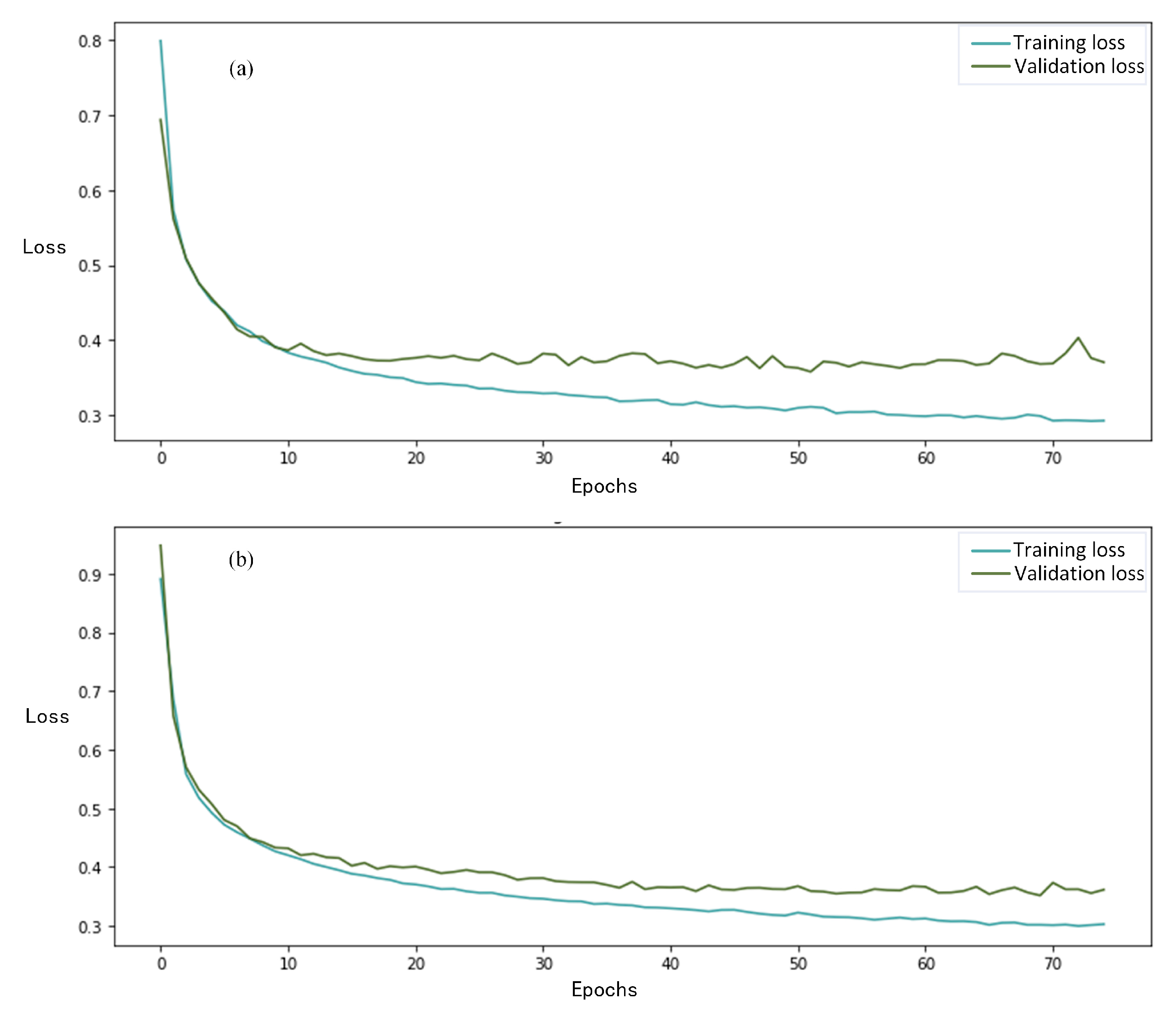
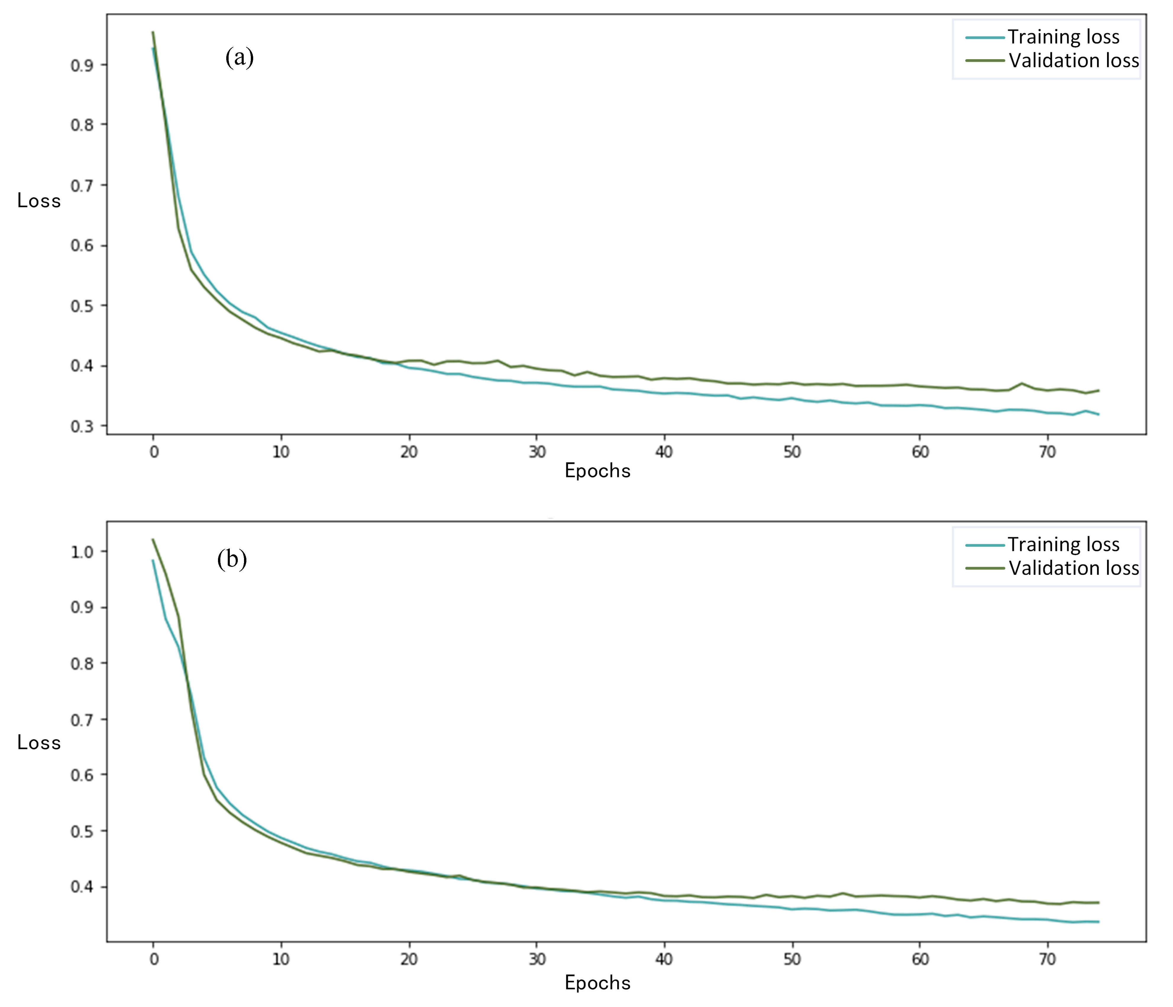
Based on the incomplete dataset, our Joint-IF model was proposed to predict the transfer passenger flow. We deployed this experimental program in Keras, a neural network application programming interface of TensorFlow, to build a completed time series processing model. As in other studies [46,47], we used the Adam optimizer and the loss function Mean Squared Error (MSE) in the Joint-IF model. Figure 4 and Figure 5 display the convergence of Joint-IF for different numbers of training samples.

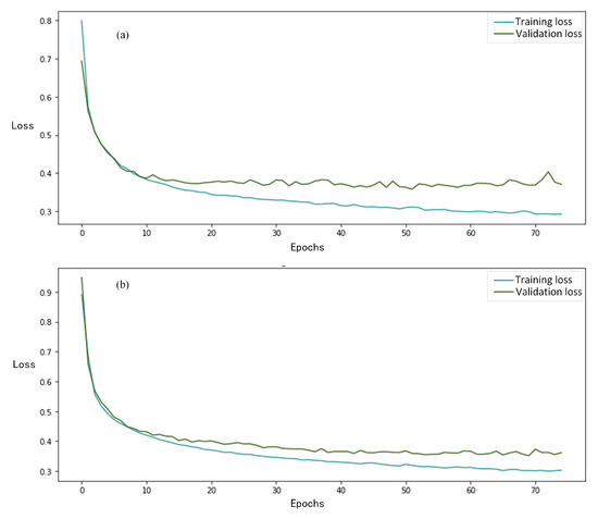
Figure 4. Convergence of the Joint-IF model using MSE with 75 iterations. (a) Batch_size = 64; (b) Batch_size = 128.

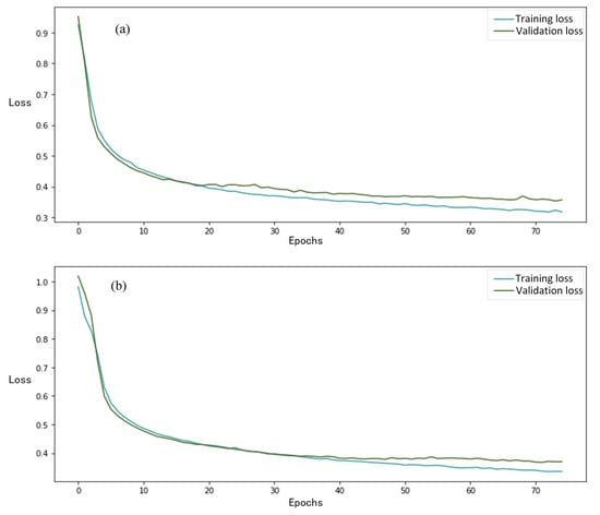
Figure 5. Convergence of the Joint-IF model using MSE with 75 iterations. (a) Batch_size = 256; (b) Batch_size = 512.

From Figure 4 and Figure 5, we can clearly see that the loss value of Joint-IF decreases sharply as the number of iterations and Batch_size increase, and Joint-IF eventually stabilizes. Thus, as shown in Table 2, we set the number of iterations and epochs to 75 and 512, respectively. In addition, as shown in Table 3, we used special settings for the structure and parameters of LSTM. Of these, to prevent the Joint-IF from over-fitting, we set the Dropout layer between the two layers.

Table 2. The parameter settings of the trained Joint-IF model.

Parameter	Settings
Loss	MSE
Optimizer	Adam
Batch_size	512
Epoch	75

Table 3. Structure and parameter settings of the LSTM network.

Numbers	Layers	Parameters	Size
1	LSTM layer	Param	3760
2	Dropout (0.1) layer	Param	0
3	LSTM layer	Param	2160
4	Dropout (0.1) layer	Param	0
5	LSTM layer	Param	2880
6	Dropout (0.1) layer	Param	0
7	Dense layer	Param	84

4.5. Experimental Results and Analysis

4.5.1. Overall Analysis

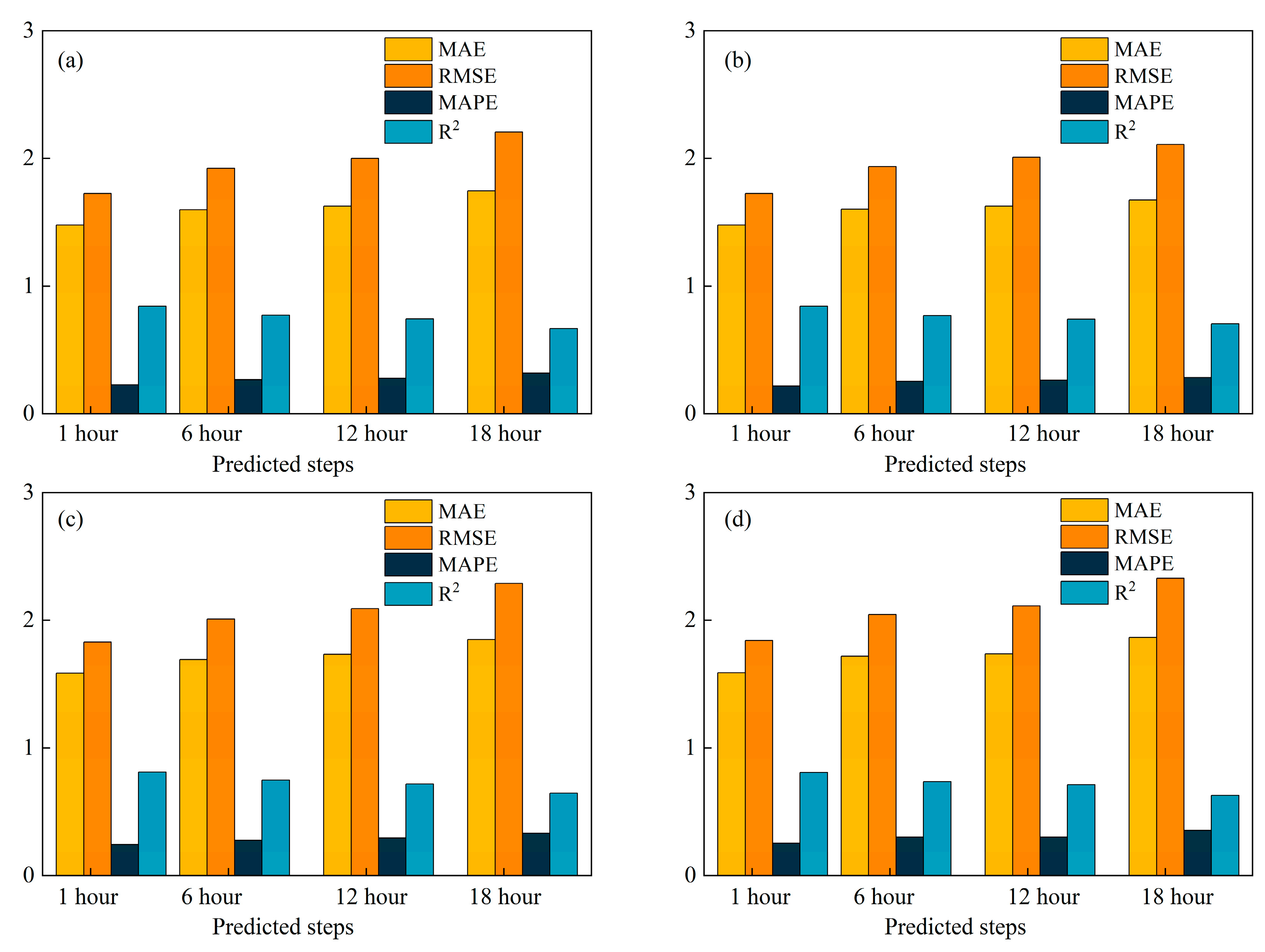
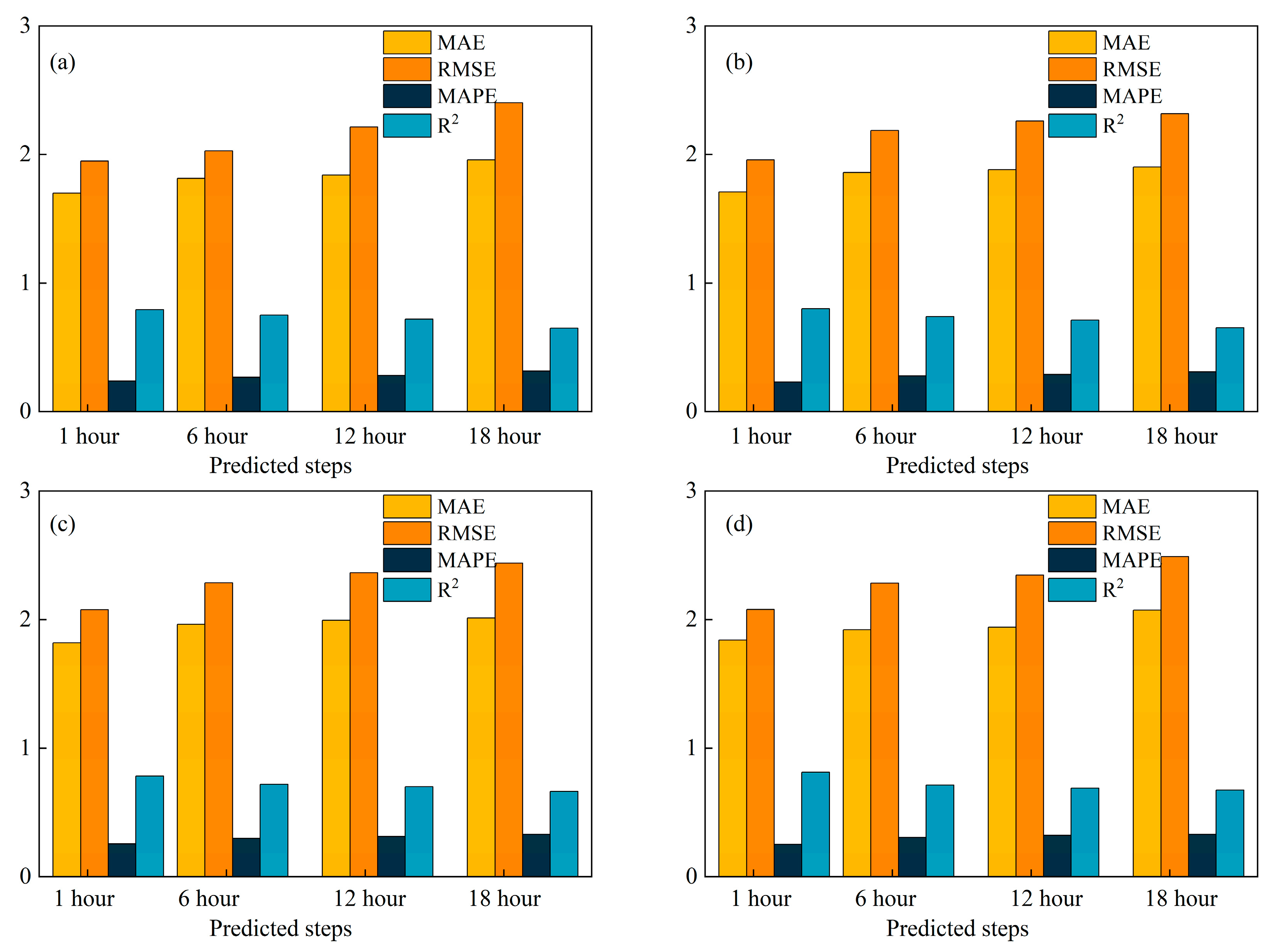
To validate the performance of Joint-IF in predicting missing transfer passenger flow, we tested the forecasting results of Joint-IF for transfer passenger flow with the combinations of RM and NM and missing ratios of 10%, 30%, 50% and 70%, respectively, and then made comparisons with those baseline models. Figure 6 and Figure 7 show four evaluation metrics of MAE, MAPE, RMSE and ${\mathrm{R}}^2$ of Joint-IF under various missing combinations for the 1, 6, 12 and 18 h forecasting tasks of transfer passenger flow at different metro stations.

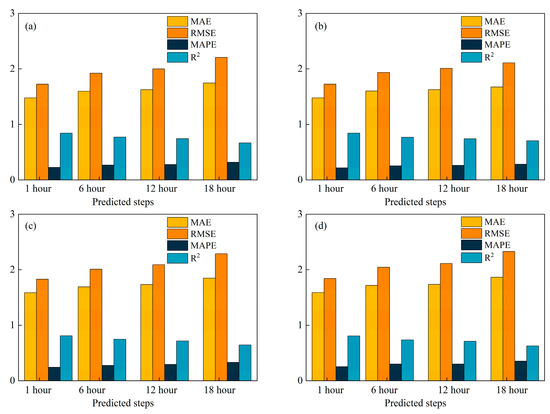
Figure 6. Measured metrics of the Joint-IF model for forecasting transfer passenger flow under various missing cases: (a) 10%, RM; (b) 10%, NM; (c) 30%, RM; (d) 30%, NM.

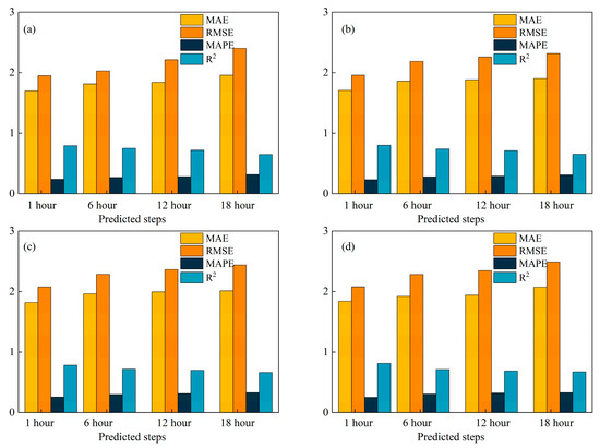
Figure 7. Measured metrics of the Joint-IF model for forecasting transfer passenger flow under various missing cases: (a) 50%, RM; (b) 50%, NM; (c) 70%, RM; (d) 70%, NM.

Comparing the prediction results of Joint-IF for transfer flow under different missing modes in Figure 6 and Figure 7, we can obtain several interesting findings:

• Under the RM and NM scenarios, the prediction errors were similar for transfer passenger flow with the same missing rates;
• The prediction errors gradually increased with the increase of missing rates, indicating the corresponding decrease of the forecasting performance. In the cases of the missing rates of 10% and 70%, it is obvious that the evaluation indexes (including MAE, MAPE and RMSE) were larger and the ${\mathrm{R}}^2$ was smaller when the missing rate was 70%;
• The differences in the forecasting results were smaller when the missing rates were small, as illustrated in Figure 6. At the missing ratios of 10% and 30%, the differences among the assessment metrics were not significant and the predicted values were relatively close.

Overall, our Joint-IF model consistently achieved favorable performance (except for the first step), although its errors increased with time interval and such tendency is accelerated. We can also observe that Joint-IF has a low forecasting error when dealing with transfer passenger flow in different missing cases, and all of the metrics show good stability and robustness.

4.5.2. Performance Comparison with Baseline Models

To further verify the superiority of the Joint-IF in predicting transfer passenger flow, we compared it against those of advanced baseline methods (i.e., MLR, GPR, GWR, RF and LSTM) for the 1 h forecasting task without loss. In Table 4, we present the performance metrics of these baselines and the Joint-IF model. It can be seen that Joint-IF can accurately estimate the transfer passenger flow with lower error and exhibit better prediction performance than those multivariate baseline models with the complete transfer passenger flow. In particular, the MAE, MAPE and RMSE of the Joint-IF model were 1.38–76.19%, 21.51–69.50% and 0.86–78.81% lower than baselines and its ${\mathrm{R}}^2$ was 2.36–65.04% higher than baselines; the GWR had the most similarity and Joint-IF the least difference.

Table 4. Performance evaluation of all models for predicting the complete transfer passenger flows.

Models	Evaluation Metrics
	MAE	MAPE	RMSE	${\mathbf{R}}^2$
MLR	2.26	0.477	2.91	0.645
GPR	6.579	0.646	8.666	0.552
GWR	1.589	0.251	1.852	0.89
RF	2.019	0.366	2.487	0.764
LSTM	1.772	0.281	2.247	0.806
Joint-IF	1.567	0.197	1.836	0.911

Comparing the forecasting results of each statistical method, it can be found that the evaluation metrics of MAE, MAPE and RMSE of GWR were significantly smaller than MLR and GPR, while ${\mathrm{R}}^2$ was larger. Therefore, among the statistical approaches, the local spatial regression models have better forecasting performance than the global regression models, and their performance is significantly improved after taking spatial location information into account. Additionally, when comparing the results of the statistical approaches, ML and DL methods in predicting complete transfer passenger flow, it was found that the ML and DL methods outperformed other statistical methods except for GWR. The LSTM model has good forecasting performance for complete transfer passenger flow. However, compared with LSTM, GWR has a smaller prediction error and better prediction performance, and GWR takes less time and has higher computational efficiency than LSTM. Further, GWR can be improved to obtain more accurate prediction results for transfer passenger flow.

Overall, the Joint-IF performed better than baselines in predicting complete transfer passenger flow and the comprehensive results also conclude that Joint-IF is capable of better forecasting transfer passenger flow with missing values between metro and bus.

4.6. Visualization Analysis

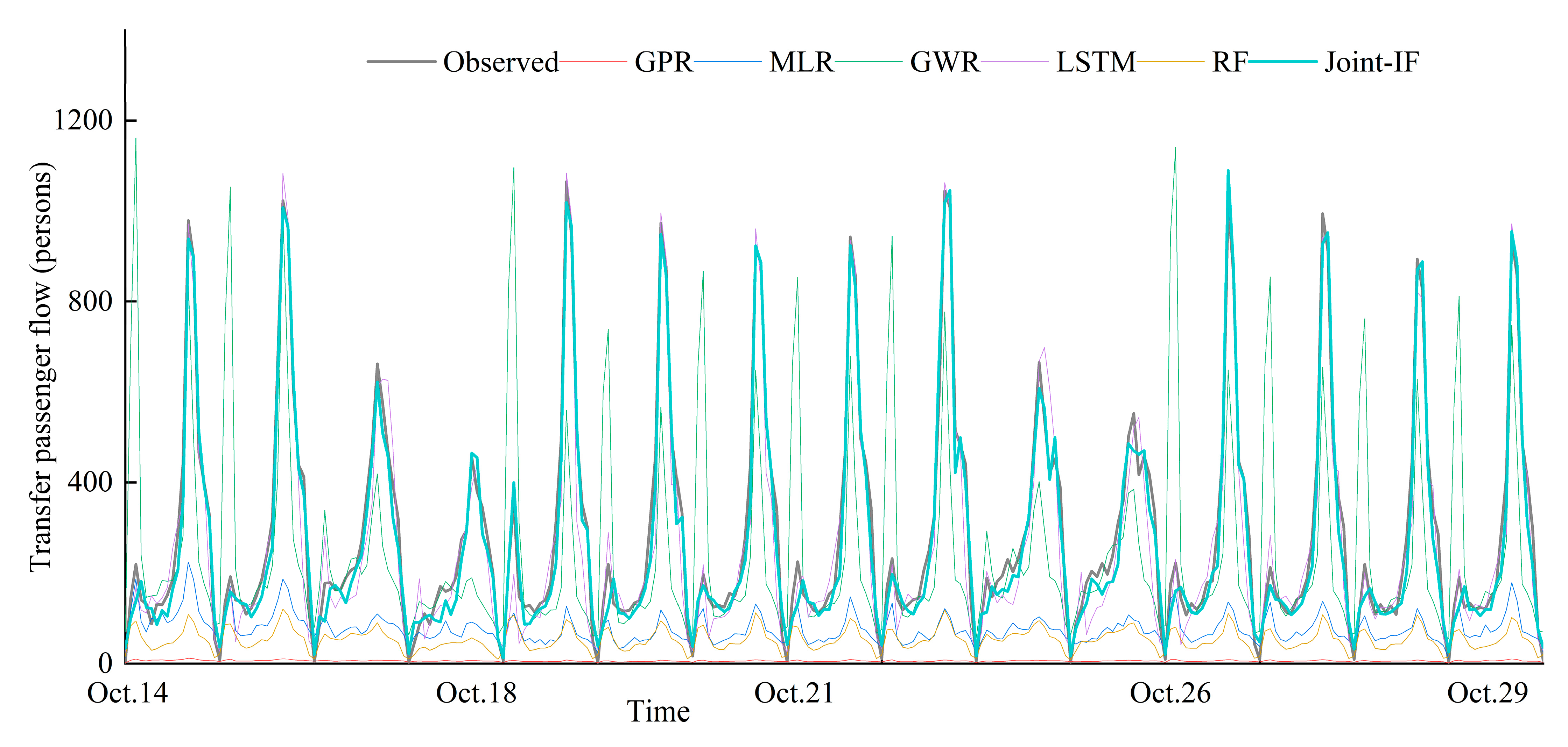
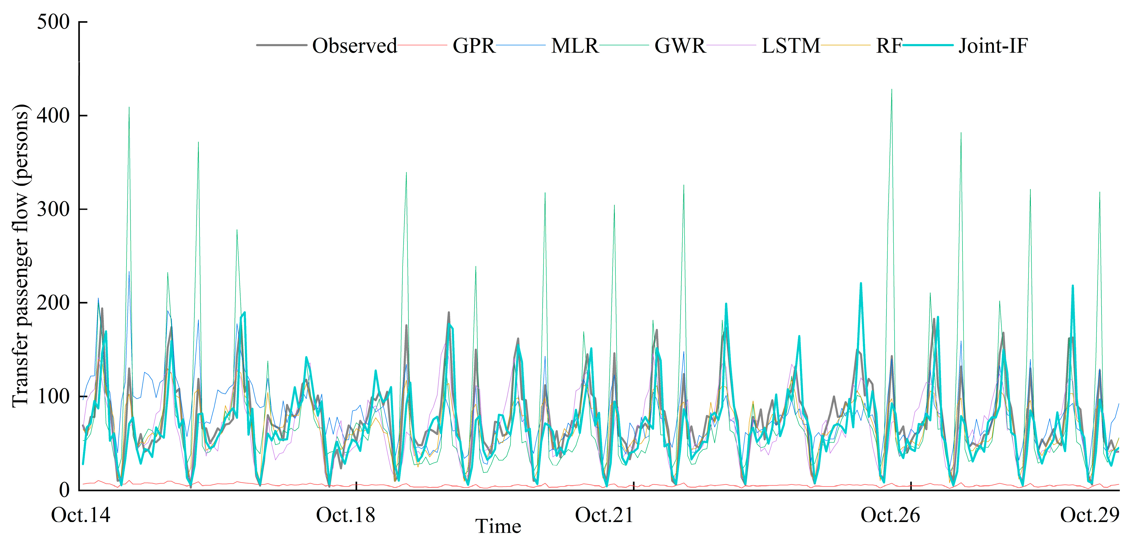
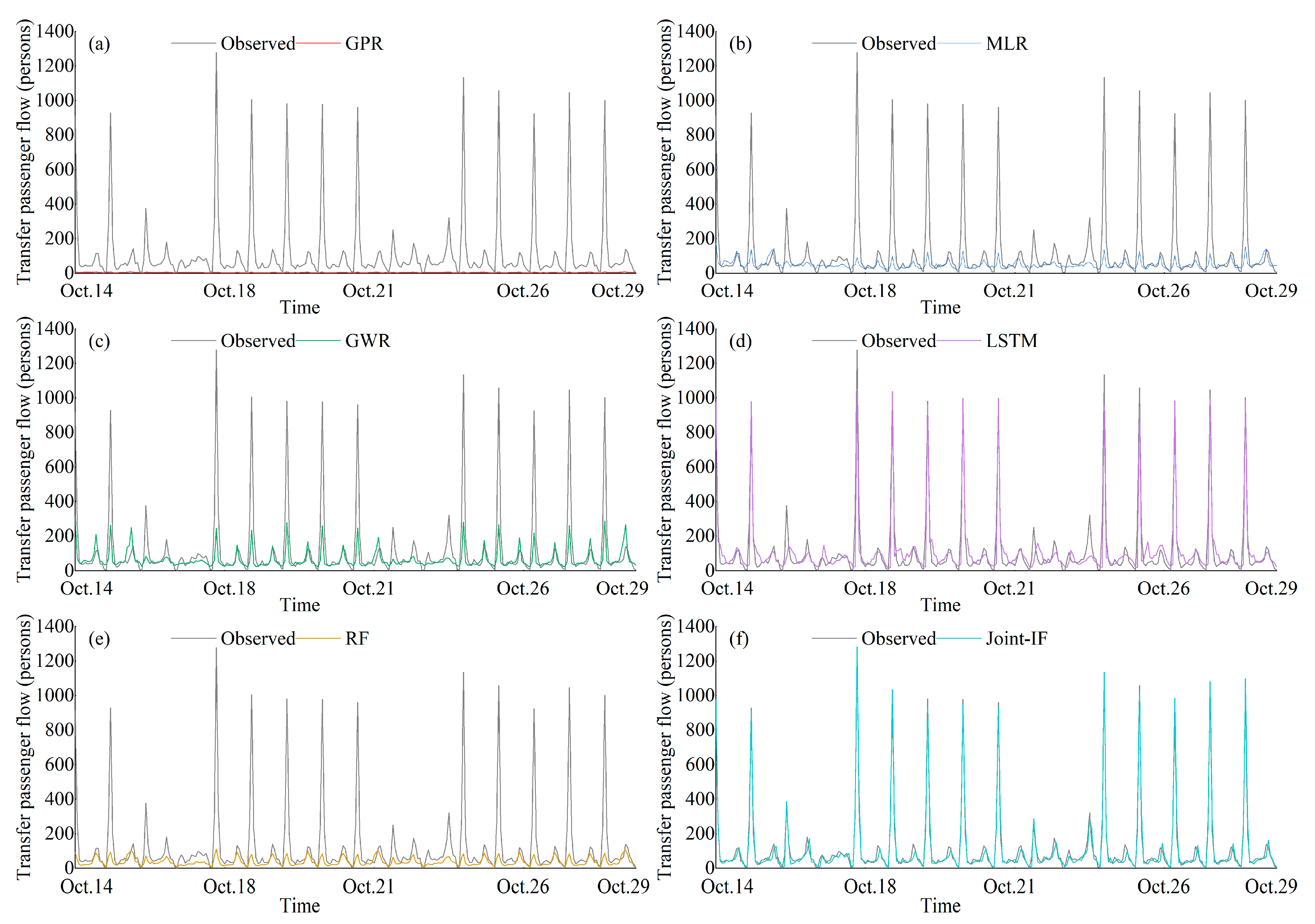
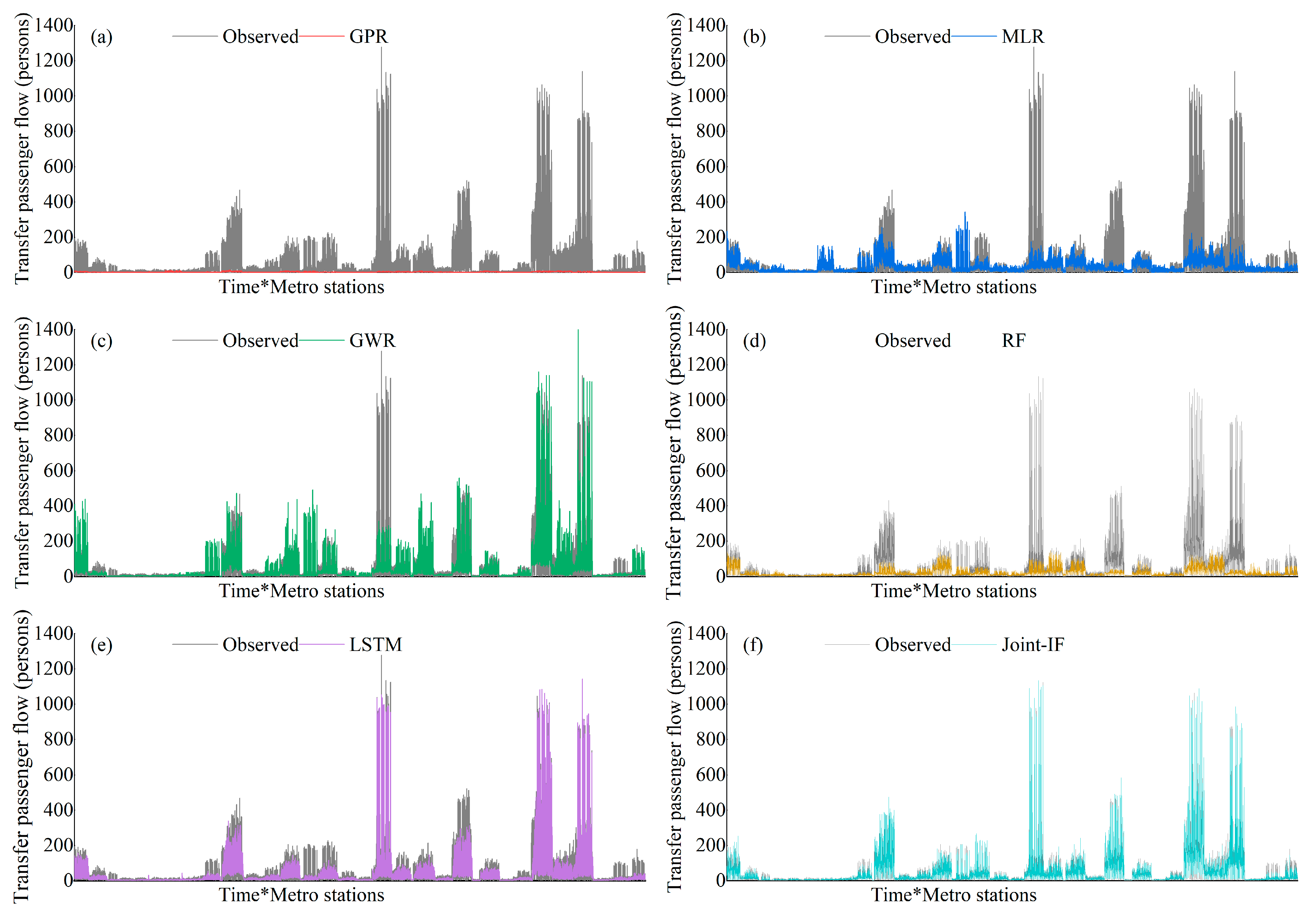
Except for the entire prediction performance as mentioned above, we have visualized and analyzed the predicted transfer passenger flow from all models with their estimations in Figure 8, Figure 9, Figure 10 and Figure 11.

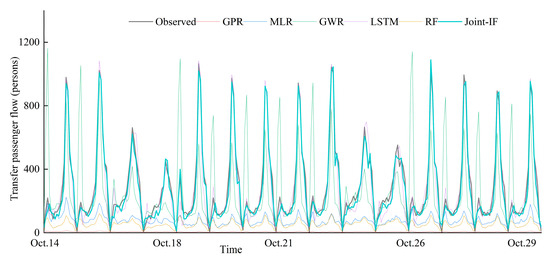
Figure 8. Predicted and true value distribution of all models for transfer passenger flow at Wuhe station.

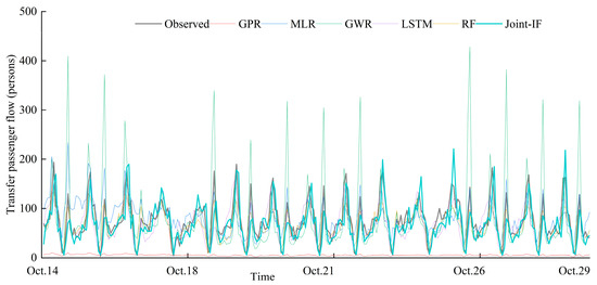
Figure 9. Predicted and true value distribution of all models for transfer passenger flow at Laojie station.

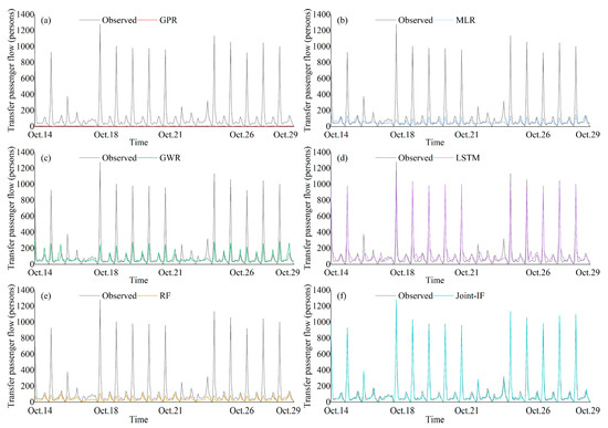
Figure 10. Predicted and true value distribution of all models for transfer passenger flow at Shenzhen North station: (a) GPR; (b) MLR; (c) GWR; (d) LSTM; (e) RF; (f) Joint-IF.

Figure 11. Predicted and true value distribution of all models for transfer passenger flow at all metro stations: (a) GPR; (b) MLR; (c) GWR; (d) LSTM; (e) RF; (f) Joint-IF.

As seen in Figure 8, Figure 9, Figure 10 and Figure 11, we can find that the distribution of transfer flow has obvious variability at different intervals and metro stations; the daily distribution of transfer flow shows significant morning and evening peaks, with typical cyclical properties. Meanwhile, there are obvious differences in the outputs of different forecasting models. Among these models, the forecasting values of Joint-IF are most similar to the corresponding true values with the smallest variations. Additionally, for different metro stations, Joint-IF can accurately prediction the periodicities and trends of the transfer passenger flow.

When comparing Figure 8, Figure 9, Figure 10 and Figure 11, it can be seen that the transfer flow of different stations has a large variability. The transfer flow of Shenzhen North metro station and Wuhe metro station was larger than of the Laojie station. When each model forecasted the transfer volume of Shenzhen North Station, the predictions fit better with the real data and can better adapt to the changing trend of transfer flow. However, at Laojie and Wuhe station, only Joint-IF obtained a better fit and other methods had significant variability with those true values. Thus, this result shows that Joint-IF can remain good forecasting performance for different stations and different orders of magnitude of transfer flow, and also forecast the changing trend of transfer flows at different scales. This is also corroborated by the predicted results in Figure 11. In other baselines, the predicted values of GWR also have better fitting performance with the true values, and its performance is closer to the Joint-IF model.

Although Joint-IF has the best forecasting performance among these methods, it does not explain the effects of each external factor on the transfer passenger flow, which is just remedied by those traditional statistical models (e.g., MLR, GPR, GWR). Nevertheless, our proposed Joint-IF model ultimately offers robust potentialities for ITS refinement because of its accurate prediction for future transfer passenger flow, such as improving service quality and supporting the transportation planning process [48].

5. Conclusions

An accurate prediction of transfer passenger flow in public transportation systems is critical for passengers and transport managers. However, the available studies do not provide accessible approaches to transfer passenger flow prediction. Moreover, it is inevitable that transfer activities are greatly affected by varied factors (e.g., weather) due to exposure to the outdoors. To address these issues, we propose a Joint-IF model to forecast the transfer passenger flows of the public transportation system when considering multiple factors. After fulfilling the repair task for incomplete transfer passenger flow, we test and compare the forecasting performance of the Joint-IF, statistical-based and DL-based models, and our core conclusions and contributions are as follows:

(1)

The Joint-IF model is capable of effectively repairing the transfer passenger flow between metro and bus under various missing combinations. Especially for those cases with large missing rates, Joint-IF can still maintain excellent repair performance, which is helpful for subsequent task of transfer passenger flow forecasting.

(2)

The Joint-IF model can accurately predict the future transfer passenger flows from metro stations to all their nearby bus stops. Compared with the baselines (e.g., GPR, GWR and MLR), Joint-IF yields greater performance gains and smaller prediction errors.

(3)

Overall, this study provides a reliable Joint-IF model for both accurate imputation and prediction of transfer passenger flow by considering the synergistic effects of multiple facts. Moreover, the visual analysis results can further confirm and explain the advantages of the Joint-IF over baselines, especially for GWR. These not only provide helpful insights for travelers and operators, but also provide a basis for later interpretable forecasting studies.

In future research, we will study the prediction of short-term transfer passenger flow (e.g., 1, 5 and 10 min intervals). Additionally, we will apply more DL-based algorithms to optimize the residuals of Joint-IF and minimize its computational complexity. Lastly, we will further explore the predictive performance of Joint-IF in other domains, such as the transfer speed of passengers.

References

- Zhang, J.L.; Chen, F.; Cui, Z.Y.; Guo, Y.N.; Zhu, Y.D. Deep learning architecture for short-term passenger flow forecasting in urban rail transit. IEEE Trans. Intell. Transp. Syst. 2020, 22, 7004–7014. [Google Scholar] [CrossRef]
- Shi, F.; Zhou, Z.; Yao, J.; Huang, H.L. Incorporating transfer reliability into equilibrium analysis of railway passenger flow. Eur. J. Oper. Res. 2012, 220, 378–385. [Google Scholar] [CrossRef]
- Shang, P.; Li, R.M.; Guo, J.F.; Xian, K.; Zhou, X.S. Integrating Lagrangian and Eulerian observations for passenger flow state estimation in an urban rail transit network: A space-time-state hyper network-based assignment approach. Transport. Res. B-Meth. 2019, 121, 135–167. [Google Scholar] [CrossRef]
- Zhang, Z.; Wang, C.; Gao, Y.E.; Chen, J.W.; Zhang, Y.W. Short-term passenger flow forecast of rail transit station based on MIC feature selection and ST-LightGBM considering transfer passenger flow. Sci. Program. 2020, 2020, 1–15. [Google Scholar] [CrossRef]
- Nuzzolo, A.; Russo, F.; Crisalli, U. A doubly dynamic schedule-based assignment model for transit networks. Transp. Sci. 2001, 35, 268–285. [Google Scholar] [CrossRef]
- Musolino, G. Sustainable mobility as a service: Demand analysis and case studies. Information 2022, 13, 376. [Google Scholar] [CrossRef]
- Sun, Y.X.; Leng, B.; Guan, W. A novel wavelet-SVM short-time passenger flow prediction in Beijing subway system. Neurocomputing. 2015, 166, 109–121. [Google Scholar] [CrossRef]
- Liu, Y.; Liu, Z.Y.; Jia, R. DeepPF: A deep learning based architecture for metro passenger flow prediction. Transp. Res. Part C Emerg. Technol. 2019, 101, 18–34. [Google Scholar] [CrossRef]
- Wen, K.Y.; Zhao, G.T.; He, B.S.; Ma, J.; Zhang, H.X. A decomposition-based forecasting method with transfer learning for railway short-term passenger flow in holidays. Expert Syst. Appl. 2022, 189, 116102. [Google Scholar] [CrossRef]
- Li, J.L.; Wu, P.; Li, R.N.; Pian, Y.Z.; Huang, Z.L.; Xu, L.H.; Li, X.C. ST-CRMF: Compensated residual matrix factorization with spatial-temporal regularization for graph-based time series forecasting. Sensors 2022, 22, 5877. [Google Scholar] [CrossRef]
- Chen, X.Y.; Sun, L.J. Bayesian temporal factorization for multidimensional time series prediction. IEEE Trans. Pattern Anal. Mach. Intell. 2021, 44, 4659–4673. [Google Scholar] [CrossRef] [PubMed]
- Tang, L.Y.; Zhao, Y.; Cabrera, J.; Ma, J.; Tsui, K.L. Forecasting short-term passenger flow: An empirical study on shenzhen metro. IEEE Trans. Intell. Transp. Syst. 2018, 20, 3613–3622. [Google Scholar] [CrossRef]
- Yin, X.Y.; Wu, G.Z.; Wei, J.Z.; Shen, Y.M.; Qi, H.; Yin, B.C. Deep learning on traffic prediction: Methods, analysis and future directions. IEEE Trans. Intell. Transp. Syst. 2021, 23, 4927–4943. [Google Scholar] [CrossRef]
- Russo, F.; Rindone, C. Smart city for sustainable development: Applied processes from SUMP to MaaS at European level. Appl. Sci. 2023, 13, 1773. [Google Scholar] [CrossRef]
- Cascetta, E. Transportation Systems Engineering: Theory and Methods; Springer Science & Business Media: Berlin/Heidelberg, Germany, 2013. [Google Scholar]
- Xing, X.X.; Zhou, X.B.; Hong, H.K.; Huang, W.H.; Bian, K.G.; Xie, K.Q. Traffic flow decomposition and prediction based on robust principal component analysis. In Proceedings of the 2015 IEEE 18th International Conference on Intelligent Transportation Systems, Las Palmas de Gran Canaria, Spain, 15–18 September 2015; pp. 2219–2224. [Google Scholar]
- Gong, Y.S.; Li, Z.B.; Zhang, J.; Liu, W.; Zheng, Y.; Kirsch, C. Network-wide crowd flow prediction of sydney trains via customized online non-negative matrix factorization. In Proceedings of the 27th ACM International Conference on Information and Knowledge Management, Torino, Italy, 22–26 October 2018; pp. 1243–1252. [Google Scholar]
- Qu, L.; Li, L.; Zhang, Y.; Hu, J.M. PPCA-based missing data imputation for traffic flow volume: A systematical approach. IEEE Trans. Intell. Transp. Syst. 2009, 10, 512–522. [Google Scholar]
- Jia, X.Y.; Dong, X.Y.; Chen, M.; Yu, X.H. Missing data imputation for traffic congestion data based on joint matrix factorization. Knowl Based Syst. 2021, 225, 107114. [Google Scholar] [CrossRef]
- Chen, L.; Thakuriah, P.; Ampountolas, K. Short-term prediction of demand for ride-hailing services: A deep learning approach. J. Big Data Anal. Transp. 2021, 3, 175–195. [Google Scholar] [CrossRef]
- Sun, B.; Sun, T.; Jiao, P.P. Spatio-temporal segmented traffic flow prediction with ANPRS data based on improved XGBoost. J. Adv. Transp. 2021, 2021, 1–24. [Google Scholar] [CrossRef]
- Mousavizadeh Kashi, S.O.; Akbarzadeh, M. A framework for short-term traffic flow forecasting using the combination of wavelet transformation and artificial neural networks. J. Intell. Transp. Syst. 2019, 23, 60–71. [Google Scholar] [CrossRef]
- Wang, S.L.; Patwary, A.U.Z.; Huang, W. A general framework for combining traffic flow models and Bayesian network for traffic parameters estimation. Transp. Res. Part C Emerg. Technol. 2022, 139, 103664. [Google Scholar] [CrossRef]
- Feng, X.X.; Ling, X.Y.; Zheng, H.F.; Chen, Z.H.; Xu, Y.W. Adaptive multi-kernel SVM with spatial–temporal correlation for short-term traffic flow prediction. IEEE Trans. Intell. Transp. Syst. 2018, 20, 2001–2013. [Google Scholar] [CrossRef]
- Lv, W.J.; Lv, Y.B.; Ouyang, Q.; Ren, Y. A bus passenger flow prediction model fused with point-of-interest data based on extreme gradient boosting. Appl. Sci. 2022, 12, 940. [Google Scholar] [CrossRef]
- Ma, X.L.; Tao, Z.M.; Wang, Y.H.; Yu, H.Y.; Wang, Y.P. Long short-term memory neural network for traffic speed prediction using remote microwave sensor data. Transp. Res. Part C Emerg. Technol. 2015, 54, 187–197. [Google Scholar] [CrossRef]
- Zhao, Z.; Chen, W.H.; Wu, X.M.; Chen, P.C.; Liu, J.M. LSTM network: A deep learning approach for short-term traffic forecast. IET Intell. Transp. Syst. 2017, 11, 68–75. [Google Scholar] [CrossRef]
- Tian, Y.; Zhang, K.L.; Li, J.Y.; Lin, X.X.; Yang, B.L. LSTM-based traffic flow prediction with missing data. Neurocomputing 2018, 318, 297–305. [Google Scholar] [CrossRef]
- Zheng, H.F.; Lin, F.; Feng, X.X.; Chen, Y.J. A hybrid deep learning model with attention-based conv-LSTM networks for short-term traffic flow prediction. IEEE Trans. Intell. Transp. Syst. 2020, 22, 6910–6920. [Google Scholar] [CrossRef]
- Khaled, A.; Elsir, A.M.T.; Shen, Y.M. TFGAN: Traffic forecasting using generative adversarial network with multi-graph convolutional network. Knowl. Based Syst. 2022, 249, 108990. [Google Scholar] [CrossRef]
- Rindone, C. Sustainable mobility as a service: Supply analysis and test cases. Information 2022, 13, 351. [Google Scholar] [CrossRef]
- Musolino, G.; Rindone, C.; Vitetta, A. Models for supporting mobility as a service (MaaS) design. Smart Cities. 2022, 5, 206–222. [Google Scholar] [CrossRef]
- Nuzzolo, A.; Comi, A. Dynamic optimal travel strategies in intelligent stochastic transit networks. Information 2021, 12, 281. [Google Scholar] [CrossRef]
- Li, J.L.; Xu, L.H.; Li, R.N.; Wu, P.; Huang, Z.L. Deep spatial-temporal bi-directional residual optimisation based on tensor decomposition for traffic data imputation on urban road network. Appl. Intell. 2022, 52, 11363–11381. [Google Scholar] [CrossRef]
- Li, J.L.; Li, R.N.; Huang, Z.L.; Wu, P.; Xu, L.H. Dynamic adaptive generative adversarial networks with multi-view temporal factorizations for hybrid recovery of missing traffic data. Neural. Comput. Appl. 2022, 35, 7677–7696. [Google Scholar] [CrossRef]
- Li, R.N.; Qin, Y.; Wang, C.H.; Li, M.Y.; Chu, X.W. A blockchain-enabled framework for enhancing scalability and security in IIoT. IEEE Trans. Ind. Inform. 2022, 2022, 3210216. [Google Scholar] [CrossRef]
- Wu, P.; Huang, Z.L.; Pian, Y.Z.; Xu, L.H.; Li, J.L.; Chen, K.X. A combined deep learning method with attention-based LSTM model for short-term traffic speed forecasting. J. Adv. Transp. 2020, 2020, 1–15. [Google Scholar] [CrossRef]
- Wu, P.; Li, J.L.; Pian, Y.Z.; Li, X.C.; Huang, Z.L.; Xu, L.H.; Li, R.N. How determinants affect transfer ridership between metro and bus systems: A multivariate generalized poisson regression analysis method. Sustainability 2022, 14, 9666. [Google Scholar] [CrossRef]
- Li, J.L.; Sun, L.J.; Li, R.N.; Lu, Y.C. Application of siSVR-Vis/NIR to the nondestructive determination of acid detergent fiber content in corn straw. Optik 2020, 202, 163717. [Google Scholar] [CrossRef]
- Li, R.N.; Qin, Y.; Wang, J.B.; Wang, H.Y. AMGB: Trajectory prediction using attention-based mechanism GCN-BiLSTM in IOV. Pattern Recognit. Lett. 2023, 169, 17–27. [Google Scholar] [CrossRef]
- Li, J.L.; Sun, L.J.; Li, Y.S.; Lu, Y.C.; Pan, X.Y.; Zhang, X.L.; Liu, Y.Y.; Song, Z.W. Rapid prediction of acid detergent fiber content in corn stover based on NIR-spectroscopy technology. Optik 2019, 180, 34–45. [Google Scholar] [CrossRef]
- Wu, P.; Xu, L.H.; Zhong, L.S.; Gao, K.; Qu, X.B.; Pei, M.Y. Revealing the determinants of the intermodal transfer ratio between metro and bus systems considering spatial variations. J. Transp. Geogr. 2022, 104, 103415. [Google Scholar] [CrossRef]
- Bae, S.; Famoye, F.; Wulu, J.T. A rich family of generalized Poisson regression models with applications. Math. Comput. Simul. 2005, 69, 4–11. [Google Scholar] [CrossRef]
- Li, W.X.; Chen, S.W.; Dong, J.S.; Wu, J.X. Exploring the spatial variations of transfer distances between dockless bike-sharing systems and metros. J. Transp. Geogr. 2021, 92, 103032. [Google Scholar] [CrossRef]
- Li, J.H.; Zhu, D.S.; Li, C.X. Comparative analysis of BPNN, SVR, LSTM, Random Forest, and LSTM-SVR for conditional simulation of non-Gaussian measured fluctuating wind pressures. Mech. Syst. Signal Process. 2022, 178, 109285. [Google Scholar] [CrossRef]
- Li, J.L.; Sun, L.J.; Li, R.N. Nondestructive detection of frying times for soybean oil by NIR-spectroscopy technology with Adaboost-SVM (RBF). Optik 2020, 206, 164248. [Google Scholar] [CrossRef]
- Ran, Z.Y.; Sun, L.J.; Liu, Y.Y.; Pan, X.Y.; Li, J.L.; Liu, Y. Forward and backward interval partial least squares method for quantitative analysis of frying oil quality. Infrared Phys. Technol. 2020, 105, 103207. [Google Scholar] [CrossRef]
- Russo, F.; Rindone, C. Regional transport plans: From direction role denied to common rules identified. Sustainability 2021, 13, 9052. [Google Scholar] [CrossRef]
Disclaimer/Publisher’s Note: The statements, opinions and data contained in all publications are solely those of the individual author(s) and contributor(s) and not of MDPI and/or the editor(s). MDPI and/or the editor(s) disclaim responsibility for any injury to people or property resulting from any ideas, methods, instructions or products referred to in the content. |
© 2023 by the authors. Licensee MDPI, Basel, Switzerland. This article is an open access article distributed under the terms and conditions of the Creative Commons Attribution (CC BY) license (https://creativecommons.org/licenses/by/4.0/).