Arsenic Contamination in Groundwater, Soil and the Food-Chain: Risk Management in a Densely Populated Area (Versilia Plain, Italy)

Abstract

This study deals with arsenic distribution in groundwater, soil and edible vegetables in the densely populated area of the Versilia Plain (Tuscany region, Italy), addressing potential impacts on people’s health. The data revealed high As concentrations in some domestic irrigation wells, exceeding 1200 µg/L. The average As concentration in topsoil and subsoil was 39 and 46 mg/kg, respectively, with the highest concentration reaching about 200 mg/kg. Arsenic concentrates in plant roots compared with the edible parts; in tomato fruits, black cabbage leaves and edible leek parts As reached about 0.2 mg/kg, 0.4 mg/kg and 3 mg/kg, respectively. Geochemical and hydrostratigraphic data suggest that As in soils and alluvial sediments originated from mineralized and historical upstream mining areas. The exposure routes for both non-carcinogenic and carcinogenic risk assessment here considered include soil ingestion, dermal absorption, soil dust inhalation and vegetable consumption. For non-carcinogenic and carcinogenic effects, the hazard was higher than the acceptance threshold. The calculated soil screening levels resulted even lower than the guideline soil-concentration imposed by Italian regulations, and this poses an issue on the actual meaning of arsenic regulatory thresholds.

1. Introduction

The aim of this study was to investigate the entity, distribution and cause of arsenic contamination in the Versilia plain in the Tuscany region of Italy and its potential impacts on human health and on the environment. Arsenic (As) is highly toxic to humans [1]; acute exposure effects range from gastrointestinal distress to death, depending on the dose, while long-term chronic exposure has been linked to cancer, cardiovascular diseases, diabetes, neurological diseases and skin lesions [2]. People may ingest As via direct routes, i.e., drinking contaminated water [3], inhaling As-contaminated dust [4] or eating contaminated food [5]. For example, As in rice from contaminated paddy fields [6] has recently been reported as one of the causes of chronic exposure with consequences to health. However, arsenic in drinkable water has the highest massive health impact; in fact, As concentration exceeding the 10 µg/L concentration threshold recommended by the World Health Organization [7] has been reported in groundwater used as drinking supply in several countries, mostly in South America and Southeast Asia, but also in West Africa [8,9,10,11,12].

Arsenic contamination is generally attributed to natural sources, such as the weathering of the most common As mineral oxides and sulfides, and/or related to specific geological settings, including hydrothermal and evaporative systems [13,14,15]. Human activities caused an increase in As contamination in the environment since arsenic has been extensively used in industry [16,17] and in agricultural chemicals [18]. Among human-caused contamination, the hot-spots of As release in past mining settings are certainly of relevance and may cause severe impacts on the environment, as well as causing health problems [19,20]. Indeed, in areas of former As-bearing ore mining and processing, various mechanisms may be responsible for the spreading of arsenic in the environment and its secondary accumulation in soils and sediments [21,22]. Arsenic released from geogenic and anthropic sources undergoes a wide range of biological and geochemical reactions in the environment [23,24]. In reducing environments, As occurs as trivalent As(III); in oxidizing aquatic environments, arsenic primarily forms negatively charged pentavalent As(V) species, even if As(III) can be maintained in oxic conditions through biological reduction [25]. Inorganic arsenic may also undergo bio-transformations, producing a number of organoarsenic and methylated species [26]. Iron, Al and Mn oxyhydroxides in soils and aquifer sediments are the primary sorbents for both inorganic As(III) and As(V) and methylated As species, due to their surface complexation properties and widespread occurrence [27,28,29,30,31,32,33]. Peat may also be responsible for As immobilization through complexation reactions [34]. Redox-sensitive species, important for As sequestration, play a critical role in As release in the subsurface. Indeed, under anaerobic conditions, reductive dissolution of Fe and Mn oxyhydroxides carrying co-precipitated or adsorbed arsenic may occur, favoring the mobilization of As to soil and sediment porewater. Arsenic in soil may be taken up by plants [35,36], adversely affecting plant metabolism and accumulating in the edible parts, posing a risk to humans and livestock.

In this context, the main objectives of the present study were: (i) to establish the spatial distribution of As in groundwater and soil and the extent of translocation to vegetables; (ii) to assess the impact of past mining activities; and (iii) to assess the non-carcinogenic and carcinogenic human health risk for children and adults exposed to arsenic in a densely populated area.

2. Geological and Hydrogeological Setting

The study area (Figure 1) was located in the Versilia plain, a 5 km wide strip of flat coastline between the Apuan Alps, a mountain range reaching almost 2000 m a.s.l., to the east–north-east and the Ligurian Sea to the west–south-west. The Versilia plain finds its natural continuation in the Apuan Riviera to the north-west, and in the Pisa plain to the south-east. The area is well-known worldwide for its tourist attraction in relation to its famous beaches and cultural heritage [37], frequented since Roman and Etruscan times, and for the famous Apuan marble extraction and processing in the territory of Carrara (Figure 1). The area is 85 km west of Florence, about 30 km north of Pisa and 25 km north-west of Lucca. The Versilia plain corresponds to the easternmost side of a large extensional basin called Viareggio Basin, which represents the post-orogenic filling of a graben structure. The sedimentation processes started in the Upper Miocene, with deposition of incoherent detrital sediments of marine origin, marine-transitional and continental. The paleogeographic evolution of the area determined the formation of a composite depositional apparatus, consisting of alluvial and palustrine sediments of different grain sizes (from pebble and gravel to silt and clay, and sometimes peat). From a hydrogeological point of view, this structure determines a complex aquifer system, with unconfined and confined aquifers arranged on several horizons, often interconnected. The aquifer structure object of this study is located at the top of this post-orogenic deposits succession.

The study area falls within the distal part of the fan of the Baccatoio stream that drains the southern portion of the Apuan Alps exposed to the sea (Figure 1). The tectonic and geological origin of the Apuan Alps is linked to the Apennine orogeny, with a mainly compressive first phase and a prevalently extensional second phase. The tectonic structure includes, from top to bottom, Tuscan Nappe, Massa Unit and Apuane Unit (metamorphic units of the Tuscan Domain), and the underlying Paleozoic metamorphic basement [38]. The carbonate rocks of the Apuan Unit (Marbles and Grezzoni Fms.) and Tuscan Nappe (mainly Calcare Cavernoso and polygenic breccias Fm., and cataclasites) host the two most important aquifer systems of the mountainous area. The medium–high permeability of these rocks and the annual rainfall of more than 2000 mm/year determine a significant groundwater flow that feeds several springs, with an average flow rate up to some tens L/s [39]. Some of these springs also feed the Baccatoio stream.

The Baccatoio stream catchment is rich with mineralization [40], especially with two main types of ore deposits: the Pb–Zn–(Ag) ore bodies, composed of galena + sphalerite + chalcopyrite ± Pb sulfosalts, and pyrite ± baryte ± iron-oxide ore bodies. Pyrite was found to be enriched in several potentially toxic elements (PTEs), particularly Tl [41] and As, with the latter reaching concentrations of about 1 g/kg. At present, there are several abandoned mine sites in the upper part of the catchment feeding acid drainages highly contaminated by PTEs, including Tl and As [42]. In particular, thallium contaminated the potable water distribution system, posing serious public health threats [43,44]).

3. Materials and Methods

3.1. Hydrostratigraphic Reconstruction

The hydrostratigraphic structure of the area was reconstructed by means of stratigraphic data obtained via 17 drillings (including cores and boreholes) available in the databases of the Tuscany Region and of local administrations. The stratigraphic sections were obtained by comparing the lithologic horizons present in every stratigraphic column. For superficial outcrops, the core data were also compared with the Geological Map of Tuscany, 1:50,000 scale (CARG Project).

3.2. Water

Groundwater was collected through 135 wells during 2018–2019 surveys (Figure 2). The wells were selected using the municipal administration database, supplemented by a door-to-door census since some wells used for groundwater abstraction were not registered. The physico-chemical parameters (temperature, electrical conductivity, pH, dissolved oxygen) were measured in the field. Total alkalinity (attributed to HCO₃⁻) was measured using acidimetric titration. For laboratory analyses, water samples were filtered to 0.45 µm and stabilized using ultrapure HNO₃ for major cation and trace determination. Major ions were determined via ion chromatography using a Thermo Fisher ICS 900. Accuracy and precision were within 5%. The concentration of a set of trace elements in water (As, Ba, Fe, Mn, Tl and Zn) was determined with ICP-MS using a Perkin Elmer NexION 300X. Deviations from the certified values of water standards NIST SRM 1640a and 1643f (20 replicates) were less than 6% for As, Ba, Mn and Tl, and 6–10% for Zn and Fe. Precision (RSD) was within 6% for As, Ba and Tl and 6–11% for Fe, Mn and Zn.

3.3. Vegetable and Soil

Sixty-three vegetable gardens were selected for soil and plant sampling during surveys conducted in 2015 and 2017 (Figure 2).

In each vegetable garden, the soil survey was carried out using an auger, collecting composite (from 4 to 5 distinct core samples) soil samples for topsoil (0–20 cm) and deeper layers (80–100 cm). Soil samples (n = 63 × 2 depths) were air-dried, sieved at <2 mm and milled to obtain ultrafine powder.

Soil samples (0.25 g) were treated with aqua regia (2 mL 65% HNO₃ + 6 mL 37% HCl, Suprapur grade) using a microwave oven (Milestone 2100). After acid digestion, the solution volumes were brought up to 20 mL with Milli-Q water and filtered with Whatman 42 filter paper. The As concentration was determined using Inductively Coupled Plasma coupled with Optical Emission Spectrometry (ICP-OES, Spectro Ametek, Kleve, Germany). The analysis of each sample was replicated three times and compared with the analysis of the International Reference Materials BCR 141 and laboratory internal standards (MO and ML) [45], which was run after every ten samples to check changes in sensitivity.

In the 2015 survey, in each vegetable garden, a composite (from four samples) for each horticultural plant, when available, was collected. The total number of samples collected was: turnip (n = 10), leek (n = 6), fennel (n = 6), onion (n = 7), tomato (fruits n = 12 and roots n = 6) and black cabbage (n = 12). In the 2017 survey, the same sampling scheme was used, but only with black cabbage (n = 48) and tomato (fruits n = 60 and roots n = 27). After washing to remove soil residues, the edible parts of vegetables and roots (i.e., turnip, leek, fennel, onion, tomato and black cabbage) were weighed and dried at 60 °C; the different parts were analyzed separately. For analysis, dry samples were ground in a blender with pure titanium blades. Both root and leaf samples (0.25 g) were treated with 6 mL of HNO₃ (Suprapur, Merck, Rahway, NJ, USA) and 2 mL of H₂O₂ (Carlo Erba, Milano, Italy) using a microwave oven (Milestone 2100). After digestion, the solution volumes were brought up to 20 mL with Milli-Q water and then filtered with Whatman 42 filter paper, and the trace elements were determined using ICP-OES (Spectro Ametek). Instrument response was assessed by measuring a standard sample (CRM 482).

3.4. Risk Analysis

Risk analysis was performed following the deterministic approach described both by ASTM standards [46] and United States Environmental Protection Agency (US EPA) guidelines [47,48,49] using Risk-net software (version 3.1.1 pro; http://www.reconnet.net/Software.htm; accessed on 26 March 2023).

The selected exposure routes were surface soil ingestion, dermal contact and soil dust inhalation. In addition, the risk of chronic exposure of the local population to potentially harmful arsenic levels through the consumption of vegetables was assessed, considering the most commonly used vegetables, i.e., tomatoes and black cabbage. Human receptors were both adults and children. Contaminated groundwater is not used for drinking purposes, and therefore it was not included in the risk analysis.

The risk for both non-carcinogenic (Hazard Quozient—HQ) and carcinogenic (R) chronic effects in humans was calculated for each exposure pathway.

The chronic daily intake (CDI, mg/kg/day) represents the exposure to a toxic agent, averaged over a long period of time, through ingestion (CDI_ing) or dermal contact (CDI_derm), given by:

$${\mathrm{CDI}}_{\mathrm{ing}}={\mathrm{C}}_{\mathrm{POE}}\times \frac{{\mathrm{R}}_{\mathrm{ing}}\times \mathrm{EF}\times \mathrm{ED} \times \mathrm{RBA}}{\mathrm{BW}\times \mathrm{AT}}\times {10}^{-6}$$

$${\mathrm{CDI}}_{\mathrm{derm}}={\mathrm{C}}_{\mathrm{POE}}\times \frac{\mathrm{SA}\times \mathrm{SAF}\times \mathrm{ABS}\times \mathrm{EF}\times \mathrm{ED}}{\mathrm{BW}\times \mathrm{AT}}\times {10}^{-6}$$

where C_POE is the exposure point concentration of the contaminant in soil (mg/kg), equal to the concentration at the source (Cs) in the case of direct exposure pathways.

For the remaining parameters, recommended values [50,51] were used: R_ing is the ingestion rate (100 mg/day for adult, 200 mg/day for children), EF is the exposure frequency (350 day/year, a value suitable for a residential setting), ED is the exposure duration (24 years for adults, 6 years for children), RBA is the relative bioavailability factor (chemical-specific, unitless, set at 0.6 for As), SA is the exposed skin area (5700 cm² for adults, 2800 cm² for children), SAF is the skin adherence factor (0.07 mg/cm² day for adults, 0.2 mg/cm² day for children), ABS is the dermal absorption factor (chemical-specific, unitless, 0.003 for As), BW is the average body weight (70 kg for adults, 15 kg for children) and AT is the average time of exposure (ED × 365 day/year for non-carcinogens, 70 year × 365 day/year for carcinogens). In the specific case of vegetable ingestion, C_POE is the metal content in the vegetable (mg/kg, fresh weight, and RBA is set equal to 1). The Ingestion Rate (R_ing = 76 gr/day for tomato and 2.5 gr/day for black cabbage) was taken from the most recent Italian food consumption survey, and it is relative to the individual daily consumption of both fresh and processed tomatoes referred to the total sample of the Italian population considered by the INRAN-SCAI 2005–2006 survey [52].

In the case of direct ingestion and dermal contact, the non-carcinogenic Hazard Quotient HQ (i.e., HQ_ingestion and HQ_dermal) was calculated by dividing the chronic daily intake by the corresponding reference dose (RfD, mg/kg/day) [51,53], defined as the maximum daily exposure to a toxic agent that would not produce any appreciable deleterious effect on human health:

$$\mathrm{HQ}=\frac{\mathrm{CDI}}{\mathrm{RfD}}$$

For the dust inhalation pathway, HQ_inhalation was calculated by dividing the exposure concentration (EC, mg/m³) by the reference toxicity concentration value (RfC, mg/m³), which represents an estimate of continuous inhalation exposure without appreciable risk of deleterious effects during a lifetime [54]:

$$\mathrm{HQ}=\frac{\mathrm{EC}}{\mathrm{RfC}}$$

where RfC was set to 1.5 × 10⁻⁵ mg/m³ [51] and EC was estimated starting from the predicted concentration in air (mg/m³) as exposure metrics, rather than inhalation intake of a contaminant in air based on the inhalation rate and an average body weight, according to:

$$\mathrm{EC}=\frac{{\mathrm{C}}_{\mathrm{POE}}\times \mathrm{ET}\times \mathrm{EF}\times \mathrm{ED}}{\mathrm{AT}}$$

Here, ET represents the exposure time (24 h/day, suitable for a residential area), AT is given by ED × 365 day/yr × 24 h/day and C_POE is the concentration in air at the exposure point (mg/m³), calculated by means of the transport model related to the dust inhalation pathway as defined by the ASTM standard [46,55].

The total non-carcinogenic risk for a single substance defines a screening level individual Hazard Index (HI_i) as:

$${\mathrm{HI}}_{\mathrm{i}}={\mathrm{HQ}}_{\mathrm{ingestion}}+{\mathrm{HQ}}_{\mathrm{dermal}}+{\mathrm{HQ}}_{\mathrm{inhalation}}$$

An HI_i value less than unity indicates that the risk is acceptable [53].

For each pathway, the carcinogenic risk (R) is defined as the incremental probability of an individual developing cancer over a lifetime resulting from exposure to the potential carcinogens [53] and is directly related to the intake:

R = CDI × SF

where the slope factor (SF) (defined as the risk generated by a lifetime average amount of one mg/kg/day of carcinogen) is the contaminant specific toxicity reference value [51], which converts the estimated daily intake averaged over a lifetime of exposure directly into the incremental risk for an individual of developing cancer.

The carcinogenic risk for soil due to direct exposure was calculated using an age-adjusted factor, namely a time-weighted average of these parameters for receptors exposed for an extended period of time (e.g., 30 years) from childhood through adulthood [48,56]. The excess cancer risk for a receptor exposed via the inhalation pathway was estimated using [54]:

$$\mathrm{R}=\mathrm{IUR}\times \mathrm{EC}$$

where IUR represents the Inhalation Unit Risk, defined as an estimate of the increased cancer risk from inhalation exposure to a given concentration (1 µg/m³) for a lifetime [51]; EC is the exposure concentration averaged over a lifetime of 70 years (AT = 70 years × 365 days/year × 24 h/day). The carcinogenic risk R_i for a single substance is represented by the sum of the contributions due to each exposure route. The permissible limits are 10⁻⁶ and 10⁻⁴ for a single carcinogenic element and multi-element carcinogens, respectively. In particular, a risk value for arsenic lower than 10⁻⁶ (one-in-a-million individual excess cancer risk) can be considered acceptable [47,48,57]. The maximum allowed concentration of contaminants in soil considered to be protective of human health (soil screening levels—SSLs, according to US EPA guidelines) was obtained by following the Risk Based Corrective Action procedure [46,47]. In this approach, the exposure equations and pathway models are run in reverse to back-calculate the acceptable level of contaminant concentration in soil corresponding to the target risk [47,56]. Risk-based SSLs for the different outdoor exposure pathways and for residential settings were derived from standardized sets of equations that are based on the updated U.S. Environmental Protection Agency’s human health risk assessment methods [56].

4. Results

4.1. Hydrostratigraphic Structure

The coastal plain can be morphologically divided into three roughly parallel bands (Figure 3). The inner one, bordering the foot of the Apuan Alps, is characterized by coalescing alluvial fans of little slope. These mainly consist of gravels, pebbles and sands, sometimes in a medium-fine matrix in the areas close to the hills, sands and silty sands in the intermediate part and silts and clays in the more distal parts. The intermediate zone includes lowland areas, in some cases even below sea level. It corresponds to ancient marshy and lagoon areas isolated from the sea by the development of a beach ridges system [58]. Most of the swampy areas have been reclaimed since the Roman times. The sediments characterizing this strip are both of a lacustrine/marshy environment, such as peats, silts and/or peaty clays, and, locally, alluvial, such as silts and clayey-sandy silts, usually with an abundant organic fraction. The coastal strip is formed by the current beach, and inwards by the system of beach ridges and coastal dunes, mostly dismantled by human action. From a sedimentary point of view, the current beach is entirely composed of medium to fine sand, as are the beach ridges and coastal dunes, of marine and windy origin, respectively.

The stratigraphic database available allowed the representation of the lithostratigraphic structure down to a depth of about 30–40 m (Figure 4).

In particular, two hydrostratigraphic sections are shown in Figure 4: one perpendicular (A-A′) and one parallel (B-B′) to the alignment of the coastal plain (see Figure 3). Section A-A′ includes the apical zone of the alluvial fan of the Baccatoio stream and is NE–SW directed, whereas section B-B′ is NW–SE directed. In the sections, the vertical scale is exaggerated compared with the horizontal scale to better appreciate narrow horizons.

In agreement with the general stratigraphic structure, three main facies were recognized:

-

deposits associated with fluvial processes, mainly consisting of coarse material (gravel) in a finer matrix (sand, silt, clay), especially in the fan area, whereas the fine matrix seems to decrease towards the SW;

-

deposits resulting from marine processes, mainly sandy with some lenses of finer grain size (silty sands);

-

mixed lacustrine and marsh deposits, consisting of mainly clayey and silty sediments, including peaty levels; these deposits can also occur as lenses within other deposits.

The alluvial fan area (section A-A′, Figure 4) is dominated by a thick, predominantly gravelly, but locally more heterogeneous, horizon, consisting of fine matrix gravels (silty and clayey sand). The average thickness investigated was about 40–50 m. In the upstream part, these deposits lie directly on the bedrock, which is found at a depth of 45 m. The main gravel horizon deepens starting from the apical area of the conoid towards the SW. Its roof was identified at a depth of about 20 m in the terminal part of section A-A′. The gravel horizon appears to locally include lenses of finer material.

However, as can be observed in section B-B′ (Figure 4), this horizon is laterally limited by finer deposits. This section also shows that the gravel horizon is surmounted by a thick and apparently continuous sandy deposit. On the other hand, it can be observed that downstream (central portion of section A-A′) the gravel horizon is surmounted by a powerful horizon (20–25 m thick) composed of sands in a finer matrix. This horizon is recognizable in a narrow band between the limit of the fan area and the intermediate band of the plain. Moreover, these deposits are confined upwards by predominantly clayey and silty materials. Finer materials are also recognizable below the sandy–silty horizon, even if the available stratigraphic data do not allow a better evaluation of the lateral continuity of these horizons. It is interesting to note that this is the area where the highest As groundwater contamination occurs (see the Discussion).

Towards the SW (section A-A′), the heterogeneous stratigraphic system seems to change to more definitely sandy deposits.

In order to characterize the subsoil of the study area from a hydrogeological point of view, hydraulic properties were qualitatively attributed to the different horizons according to the following criteria:

-

aquifers—mainly gravelly and sandy horizons (sky blue color in sections A-A′ and B-B′);

-

aquitards—gravels in silty and silty–clayey matrix; silty sands, sandy peats, sandy silts; gravelly silts (light sky blue color in sections A-A′ and B-B′);

-

aquicludes—predominantly clayey and clayey–silty and peaty deposits (yellow color in sections A-A′ and B-B′).

4.2. Water Chemistry

The physico-chemical parameters and major ion chemistry of groundwater are reported in

Table 1. Physico-chemical parameters and concentration of major ions in groundwater in most of the wells from W1 to W172.

Sample	Deep (m)	T (°C)	HCO3− (mg/L)	pH	O2 (mg/L)	EC (µS/cm)	Na+ (mg/L)	K+ (mg/L)	Mg2+ (mg/L)	Ca2+ (mg/L)	Cl− (mg/L)	NO3− (mg/L)	SO42− (mg/L)	NH4+ (mg/L)
W-2	n.d	18	368	6.8	3.4	637	15.5	2.6	17.4	96	25.3	4.1	33	0.05
W-3	6.0	19.1	326	7.1	n.d	609	22.9	1.9	15.8	86	34	5.0	40	0.06
W-4	n.d	17.8	226	7.0	n.d	579	20.2	1.7	14.1	81	34	5.5	35	0.05
W-5	29.0	17.2	171	7.3	n.d	7460	1313	54	159	126	2305	5.0	219	2.40
W-6	n.d	18.6	338	7.1	n.d	739	20.9	4.1	20.7	112	38	13.3	34	0.05
W-7	30.0	16.8	271	7.4	n.d	520	12.5	1.9	8.4	85	17.8	5.6	43	0.05
W-8	15.0	18.5	300	7.0	n.d	646	18.1	3.6	16.9	101	27.9	12.3	37	0.05
W-9	20.0	17.3	294	7.1	n.d	687	17.4	2.4	15.4	107	28.0	15.7	38	0.05
W-10	30.0	18.5	354	7.5	n.d	641	15.5	2.6	17.4	96	25.3	4.1	33	0.05
W-11	38.0	18.1	303	7.0	n.d	638	15.8	1.7	11.7	105	24.2	13.8	43	0.05
W-12	40.0	16.9	276	7.3	n.d	624	15.2	1.6	11.9	100	22.3	12.6	42	0.05
W-13	12.0	19.3	377	7.3	n.d	1275	70	7.5	23.5	159	152	1.3	59	0.18
W-14	n.d	17.8	285	7.1	n.d	564	16.6	5.1	16.8	76	19.3	0.50	27.6	0.12
W-15	n.d	15.7	287	7.6	1.3	365	22.0	9.6	12.9	71	30	1.5	20.0	n.d
W-16	6.0	18.1	331	8.1	n.d	620	26.1	4.6	13.4	86	15.4	1.0	22.1	0.05
W-17	6.0	17.2	288	8.1	n.d	664	26.4	6.0	16.0	92	25.3	11.9	63	0.06
W-18	n.d	16.8	328	8.0	n.d	597	13.4	8.1	18.8	83	16.4	6.9	35	0.05
W-19	6.0	16.7	298	7.6	n.d	710	22.8	7.9	15.6	99	33.3	21.8	37	3.10
W-20	8.0	18.1	377	7.3	n.d	638	13.5	1.8	18.3	96	23.6	0.50	20.5	0.12
W-21	6.0	15.9	287	7.9	n.d	673	14.9	9.0	20.1	93	27.2	9.5	59	0.05
W-22	7.0	17.9	246	7.1	n.d	456	14.6	0.8	12.3	70	17.8	3.7	30	0.05
W-23	5.0	16.7	316	7.3	n.d	664	15.7	2.2	20.0	96	25.6	0.50	26.5	0.10
W-24	8.0	17.2	598	7.7	n.d	994	26.8	4.1	28.7	150	38.8	0.60	20.4	0.92
W-25	28.0	15.9	285	7.5	n.d	574	13.0	2.8	11.1	95	19.3	9.8	46	0.05
W-26	7.0	18.4	362	7.0	n.d	1547	149	6.8	31.1	157	138	2.0	264	2.60
W-27	8.0	19.3	614	7.3	n.d	1277	66	23.0	76.6	105	68	1.0	114	0.76
W-28	8.0	17.1	302	7.7	n.d	567	15.4	4.9	22.1	75	20.6	0.5	27.5	0.15
W-29	60.0	17.7	298	8.7	n.d	558	13.1	1.3	9.7	99	19.5	10.1	55	0.05
W-30	8.0	19.2	341	6.8	n.d	1426	31	7.0	51	245	35	1.0	440	1.20
W-31	50.0	17.8	270	7.6	n.d	632	17.2	1.8	10.0	102	31	9.7	73	0.05
W-32	n.d	19	454	7.1	7.0	757	12.4	14	16.2	120	20.2	12.6	17.6	0.84
W-33	50.0	16.9	302	7.5	n.d	594	11.3	2.0	13.9	103	15.6	1.2	46	0.05
W-34	39	16.5	271	7.9	2.6	387	49	5.9	9.3	48	35	0.36	4.0	n.d
W-35	28.0	15.6	316	6.8	n.d	716	15.6	2.4	15.5	118	22.7	8.2	47	0.10
W-36	12.0	18.7	306	7.6	n.d	630	30	11.8	38	44	25.0	0.50	46	0.62
W-37	28.0	18.2	370	7.3	7.7	600	15.6	2.4	15.5	118	22.7	8.2	47	n.d
W-39	7.0	16.9	435	7.0	n.d	869	22.8	1.8	16.5	151	22.3	19.6	48	0.10
W-40	n.d	19.1	297	7.3	n.d	825	67.8	16.0	23.4	79	90	1.0	57	0.32
W-41	10.0	18.7	31	7.2	4.8	599	17.9	4.3	24.9	127	302	n.d	7.4	1.3
W-42	10.0	16.7	503	7.3	n.d	859	17.9	4.3	24.9	127	30	1.0	7.4	1.30
W-43	11.0	17.2	362	7.2	n.d	720	14.4	1.7	20.3	111	24.9	0.50	15.8	0.11
W-45	39.0	16.9	270	7.4	n.d	505	13.7	1.6	12.3	74	14.8	0.50	10.5	0.49
W-46	8.0	16.2	351	7.0	n.d	1584	70	9.0	31.9	234	127	1.0	303	0.94
W-47	46	14.7	251	7.7	5.0	659	13	6.5	12.7	87	18.51	n.d	42	n.d
W-48	35	15.3	302	7.0	6.4	471	60	2.7	11.3	39	19.7	0.85	0.25	n.d
W-49	n.d	14.3	364	6.7	5.4	594	17	5.9	9.1	116	21.1	8.37	17.0	n.d
W-51	22	15.7	299	7.7	1.1	363	15	4.0	12.9	78	13.7	0.29	12.0	n.d
W-53	9.0	18.2	514	7.1	n.d	835	16.4	2.1	23.3	127	31	1.0	2.4	1.70
W-57	25	15.1	256	7.6	7.5	391	12	1.7	10.3	106	19.1	12.2	69	n.d
W-59	16.0	14.2	341	7.0	n.d	741	18.3	1.4	13.5	126	20.6	26.8	35	0.10
W-62	25.0	15.8	309	7.4	n.d	627	12.3	1.4	11.1	106	18.3	11.6	74	0.05
W-67	23	15.3	345	6.4	2.8	640	13	4.7	17.5	105	23.9	10.3	63	n.d
W-69	20	18.1	329	7.5	n.d	630	12.3	1.5	13.7	128	17.6	11.0	71	0.05
W-71	22.0	18.2	301	7.0	n.d	684	16.0	2.0	15.2	109	22.6	9.7	56	0.05
W-81	51.0	17.4	280	6.9	n.d	683	21.2	2.6	8.9	108	37	22.4	64	0.10
W-84	11.0	13.4	386	7.0	7.3	619	19.4	2.0	18.7	123	29.4	4.8	52	4.1
W-87	9.0	15.7	396	7.0	6.5	603	12	5.0	17.3	107	22.3	n.d	10.0	n.d
W-91	7.0	23	413	7.0	1.3	829	17.5	23.4	27.4	103	19.2	n.d	68	n.d
W-95	57	15.5	306	6.9	4.8	672	13	10.3	3.7	100	20.2	18.5	26	n.d
W-96	12.0	15.6	312	6.7	5.4	650	18	4.8	8.5	117	25.5	12.6	35	n.d
W-98	25.0	16.1	223	7.5	6.9	404	11	1.5	10.1	103	16.9	9.7	77	n.d
W-103	12.0	16.5	246	6.6	2	720	12	4.3	16.4	107	22.8	7.9	95	n.d
W-110	23.0	17.9	303	7.1	n.d	628	12.4	1.2	10.5	105	18.6	11.0	74	0.07
W-111	9.0	15.9	304	6.9	6.2	585	11	6.0	16.5	97	21.8	0.96	61	n.d
W-116	36	15.1	212	6.9	8.4	578	11.3	3.9	10.2	95	17.5	7.5	75	n.d
W-118	21.0	18.2	231	7.1	n.d	605	12.3	2.1	10.5	104	18.8	12.2	65	0.05
W-124	9.0	15.7	541	7.3	3.8	808	14.4	1.9	20.8	132	20.0	n.d	3.9	1.0
W-126	22.0	17.1	317	7.4	n.d	659	17.1	7.5	15.3	102	21.6	1.0	43	1.5
W-132	30.0	16.8	254	7.0	n.d	638	12.6	2.0	10.3	93	20.0	8.0	81	0.05
W-133	18.0	18.2	206	7.5	n.d	674	9.9	1.5	11.6	91	16.6	4.0	103	0.05
W-140	25.0	13.4	204	7.3	7.1	859	10.6	1.5	10.9	100	16.7	8.6	88	n.d
W-147	n.d	15.9	231	6.9	8.5	709	11.0	1.1	12.2	122	16.9	8.7	131	0.8
W-157	10.0	17.8	329	7.6	n.d	587	15.5	2.2	14	117	22.9	7.2	51	n.d
W-160	66.0	16.6	254	7.0	n.d	520	13.3	2.3	7.0	84	21.1	13.2	18.8	0.05
W-163	66	15.5	329	6.9	8.4	550	15.0	3.3	5.9	101	22.8	13.4	19.0	n.d
W-164	66	15.8	310	7.1	n.d	578	14.5	1.9	6.1	100	23.4	14.1	19.5	0.05
W-165	8.0	13.3	260	6.9	8.3	594	10.0	7.2	11.2	89	21.2	6.7	76	n.d
W-166	67	15.4	248	6.6	4.3	547	16.0	4.1	13.1	77	26.2	5.0	57	n.d
W-167	5.0	13.6	237	6.6	8.1	523	11.0	3.2	12.0	94	22.7	7.3	90	n.d
W-168	37	17.2	31	5.9	n.d	187	14.4	0.20	3.2	15	24.3	11.9	20.3	0.05
W-169	9.0	15.3	232	6.6	4	583	14.0	5.5	12.9	100	26.8	7.4	97	n.d
W-170	72	16.1	305	7.2	n.d	879	19.6	1.4	24.7	138	27.3	1.8	207	0.10
W-171	8.0	15.2	246	6.6	6.6	438	12.0	6.0	5.5	77	18.3	10.7	22.0	n.d
W-172	n.d	15.7	234	6.9	8.2	641	11.0	7.7	7.9	93	21.4	18.3	53	n.d

n.d = not determined.

. pH values ranged from circum-neutral to alkaline (in the range from 5.9 to 8.1); dissolved oxygen (DO) was in the 1.1–8.5 mg/L range, indicating that the spatial structure of the aquifer ranges from hypoxic conditions, with DO content strongly below saturation due to an oxygen consumption rate exceeding the supply of oxygenated water, to slightly undersaturated in atmospheric oxygen. Electrical conductivity (EC) data spanned a broad range of values (between 187 µS/cm and 7460 µS/cm); total dissolved solids, TDS, were between 112 and 4265 mg/kg. The major ion composition of groundwater plotted in the Piper diagram (Figure 5) indicates a Ca-HCO₃-type composition for most groundwater samples; some samples belong to the Mg-HCO₃ (W-27, W-36), NaHCO₃ (W-48), Ca-Cl (W-41, W-168), Ca-SO₄ (W-30, W-46) and Na-Cl (W-5) hydrofacies. These data suggest the possible effects of cation exchange in the aquifer. However, for the W-5 sample, belonging to the coastal area, the possible role of seawater intrusion has been addressed by coupling chloride and boron content, assumed as conservative tracers. In particular, the B content in W-5 was 600 µg/L. Considering the average seawater composition, about 13% of the seawater component for both elements was obtained. Although further investigations are required, the data suggest that the Na-Cl hydrofacies of W-5 is attributable to marine intrusion.

The concentrations of As, Ba, Fe, Mn, Tl and Zn are reported in

Table 2. Considered trace elements’ concentration in most of the groundwater from W1 to W172 wells together with the maximum concentration level (MCL, µg/kg) imposed by Italian regulations for groundwater. Values in bold exceed the MCL.

Sample	Mn (µg/L)	Zn (µg/L)	Ba (µg/L)	Tl (µg/L)	Fe (µg/L)	As (µg/L)
MCL	50	3000		2	200	10
W-1	4.0	574	50	0.05	23	1.0
W-2	1.0	87	235	<0.05	<15	1.7
W-3	6.3	25	106	0.05	20	1.8
W-4	1.0	25	82	0.05	<15	1.1
W-5	242	49	24	0.05	866	4.2
W-6	1.4	16.0	93	0.05	<15	1.3
W-7	9.9	826	93	0.61	<15	1.0
W-8	1.0	241	201	0.05	<15	2.1
W-9	1.0	22	267	0.05	<15	1.0
W-10	1.0	87	235	0.05	<15	1.7
W-11	2.1	17.0	326	0.05	<15	2.4
W-12	1.1	23	349	0.05	<15	2.7
W-13	303	159	20	0.05	402	1.0
W-14	230	45	203	0.05	1428	59
W-15	0.46	202	0.55	0.04	366	2.6
W-16	258	148	31	0.05	62	1.0
W-17	231	49	2.9	0.05	45	2.1
W-18	137	15.0	2.2	0.05	<15	1.0
W-19	335	11.0	8.8	0.05	31	1.4
W-20	200	22	128	0.05	150	1.0
W-21	253	14.0	18.0	0.05	173	3.6
W-22	5.3	209	69	0.05	33	1.0
W-23	127	14.0	290	0.05	708	2.5
W-24	99	4.3	148	0.05	677	1.0
W-25	1.0	462	195	0.05	<15	2.6
W-26	527	223	5.3	0.05	6465	102
W-27	590	189	6.6	0.05	1880	24
W-28	54	88	5.0	0.05	487	1.0
W-29	1.0	5.0	244	0.05	<15	1.8
W-30	898	43	18.0	0.05	2585	5.7
W-31	1.0	8.2	131	0.05	<15	1.2
W-32	454	539	16	<0.05	<15	1.4
W-33	43	16.0	118	0.05	48	1.5
W-34	193	38	0.61	0.06	1313	1103
W-35	7.8	62	233	0.05	260	2.7
W-36	76	15.0	4.0	0.05	213	2.8
W-37	8.9	66	237	<0.05	255	2.6
W-38	762	123	2.6	<0.05	9750	27
W-39	5.9	12.0	199	0.05	<15	1.0
W-40	23	238	71	0.05	459	247
W-41	56	36	91	0.10	59	1.4
W-42	55	30	80	0.10	29	1.3
W-43	159	261	242	0.05	2725	1.0
W-45	495	73	512	0.05	4240	249
W-46	1770	40	16.0	0.05	6390	13.0
W-47	0.47	26	n.d	0.02	2635	153
W-48	133	141	1205	0.05	238	107
W-49	12.6	29	58	0.04	161	5.4
W-50	12.0	60	145	0.05	<15	1.5
W-51	0.45	75	0.53	0.02	1673	117
W-53	105	132	442	<0.05	1219	1.0
W-54	63	15	290	<0.05	68	224
W-55	207	59	1802	<0.05	1814	1274
W-56	25	68	169	0.12	181	1.0
W-57	0.93	42	111	0.05	59	2.3
W-58	439	13	37	<0.05	4152	140
W-59	1.0	6.4	238	0.05	<15	1.3
W-60	25	68	169	0.12	181	1.0
W-61	2.7	335	222	0.05	<15	1.6
W-62	1.0	15.0	98.0	0.05	<15	2.5
W-64	638	16	1755	<0.05	2170	798
W-65	12	60	145	<0.05	<15	1.5
W-66	171	2.9	75	<0.05	2570	32
W-67	0.76	62	289	0.02	54	2.7
W-69	<1	23	116	<0.05	<15	1.0
W-70	437	77	591	<0.05	3140	162
W-71	1.0	2613	264	0.05	<15	1.0
W-72	<1	274	145	<0.05	<15	2.1
W-74	1565	69	630	<0.05	2102	117
W-76	<1	189	109	0.13	<15	1.0
W-77	1.8	65	225	0.07	<15	1.8
W-80	12	4800	137	<0.05	<15	1.0
W-81	1.0	100	159	0.05	<15	1.0
W-83	338	80	14	<0.05	483	1.0
W-84	233	32	629	<0.05	14,290	11.0
W-86	140	61	4.4	<0.05	1464	1.3
W-87	125	n.d	5.4	0.02	332	0.7
W-88	<1	8.00	216	0.18	<15	1.9
W-90	<1	40	268	0.08	<15	1.6
W-91	521	19	15	<0.05	94	1.1
W-92	25	52	278	<0.05	209	1.0
W-94	25	60	273	<0.05	218	1.0
W-95	1.4	<9	14.3	0.01	56	0.1
W-96	3.6	13.5	239	0.13	79	1.2
W-97	2.0	23	277.0	0.11	15.0	1.8
W-98	0.2	39	97	0.09	62	1.8
W-99	2.2	25	278	0.11	<15	1.6
W-102	117	2	47	<0.05	1160	1.0
W-103	2.1	32	74	0.03	59	0.3
W-104	4.7	1434	127	0.13	169	1.0
W-106	<1	26	165	<0.05	<15	1.7
W-108	4.2	66	120	<0.05	53	1.3
W-110	55	2195	108	<0.05	17	1.0
W-111	101	9.6	6.0	0.01	110	0.1
W-114	<1	35	109	<0.05	<15	1.0
W-115	<1	87	103	0.07	<15	2.0
W-116	0.18	10.7	115	0.14	51	1.9
W-117	3.2	323	89	<0.05	<15	2.1
W-118	3.6	203	113	0.05	15.0	1.3
W-121	<1	17	93	0.07	27	1.9
W-122	13	115	110	0.1	<15	2.2
W-124	53	1.7	6.1	<0.05	33	1.0
W-126	132	5.1	183	0.05	297	15.0
W-128	<1	9.3	67	0.1	<15	1.2
W-129	<1	17	75	<0.05	<15	1.2
W-131	6.4	568	110	<0.05	434	1.9
W-132	<1	8.2	139	0.15	<15	2.4
W-133	4.0	273	83	0.1	30	1.0
W-134	2.5	6.6	104	0.14	48	2.0
W-136	45	82	35	<0.05	887	20.0
W-138	<1	53	79	0.11	<15	1.2
W-140	80	5.8	543	<0.05	861	1.0
W-142	<1	43	246	0.07	<15	1.0
W-145	<1	82	68	<0.05	<15	1.4
W-146	<1	145	40	<0.05	<15	1.0
W-147	<1	10.0	115	0.07	17	1.7
W-149	109	7.6	384	<0.05	160	1.0
W-150	<1	133	41	<0.05	26	1.0
W-152	1.2	538	108	<0.05	<15	1.0
W-153	4.0	122	85	0.07	115	1.0
W-155	109	76	384	0.05	160	1.0
W-157	4.0	1477	263	<0.05	283	1.9
W-158	142	23	103	<0.05	1730	1.0
W-160	<1	38	30	0.05	<15	1.0
W-161	<1	301	73	<0.05	<15	1.7
W-163	0.36	n.d	39	0.03	44	0.6
W-164	4.1	35	40	0.05	<15	1.0
W-165	1.2	26	61	0.06	52	1.7
W-166	3.5	18.9	99	0.1	75	2.9
W-167	1.3	19.3	71	0.13	67	1.6
W-168	16.0	12.0	60	0.05	162	1.0
W-169	1.6	n.d	88	0.19	57	1.8
W-170	1.4	27	30	0.05	46	1.0
W-171	60	74	168	0.51	80	1.3
W-172	8.6	695	177	0.63	59	2.9

n.d = not determined.

. Among trace metals, Fe and Mn ranged from <15 to 14,290 and from <1 to 1770, respectively. High Fe and Mn concentrations are commonly found in groundwater in these settings and have been attributed to geogenic sources. Barium ranged between 0.5 and 1800 µg/L; Zn ranged between 1.7 and 4800 µg/L. Thallium was present in very low concentrations in all samples, indicating that the contamination deeply affecting the Baccatoio stream water did not reach the depths of the groundwater. Arsenic reached the exceedingly high value of 1274 µg/L. It must be noted that these elements reflect the mineralization and past mining works’ acid drainages in the Baccatoio stream basin; in particular, speciation analysis (Geochemist’s Workbench^®) indicates that As in groundwater occurs mostly as As(OH)₃ or HAsO₄²⁻ species, depending on redox conditions. It is also worth noting that As(III) is generally considered more toxic and mobile than pentavalent arsenate. Saturation indices show that waters approach saturation with calcite, dolomite and witherite; some samples (W-34, W-48, W-51 and W-84, among those with As exceeding the 10 µg/L threshold) were strongly supersaturated with Mn-oxides (birnessite, pyrolusite, todorokite and hausmannite) and Fe-oxyhydroxides (hematite, goethite and ferrihydrite). The log f_CO2 calculated on the basis of carbonate equilibria ranged between −1.3 and −2.6, exceeding the air-saturated value and indicating that carbon in organic matter in the aquifer is oxidized to CO₂.

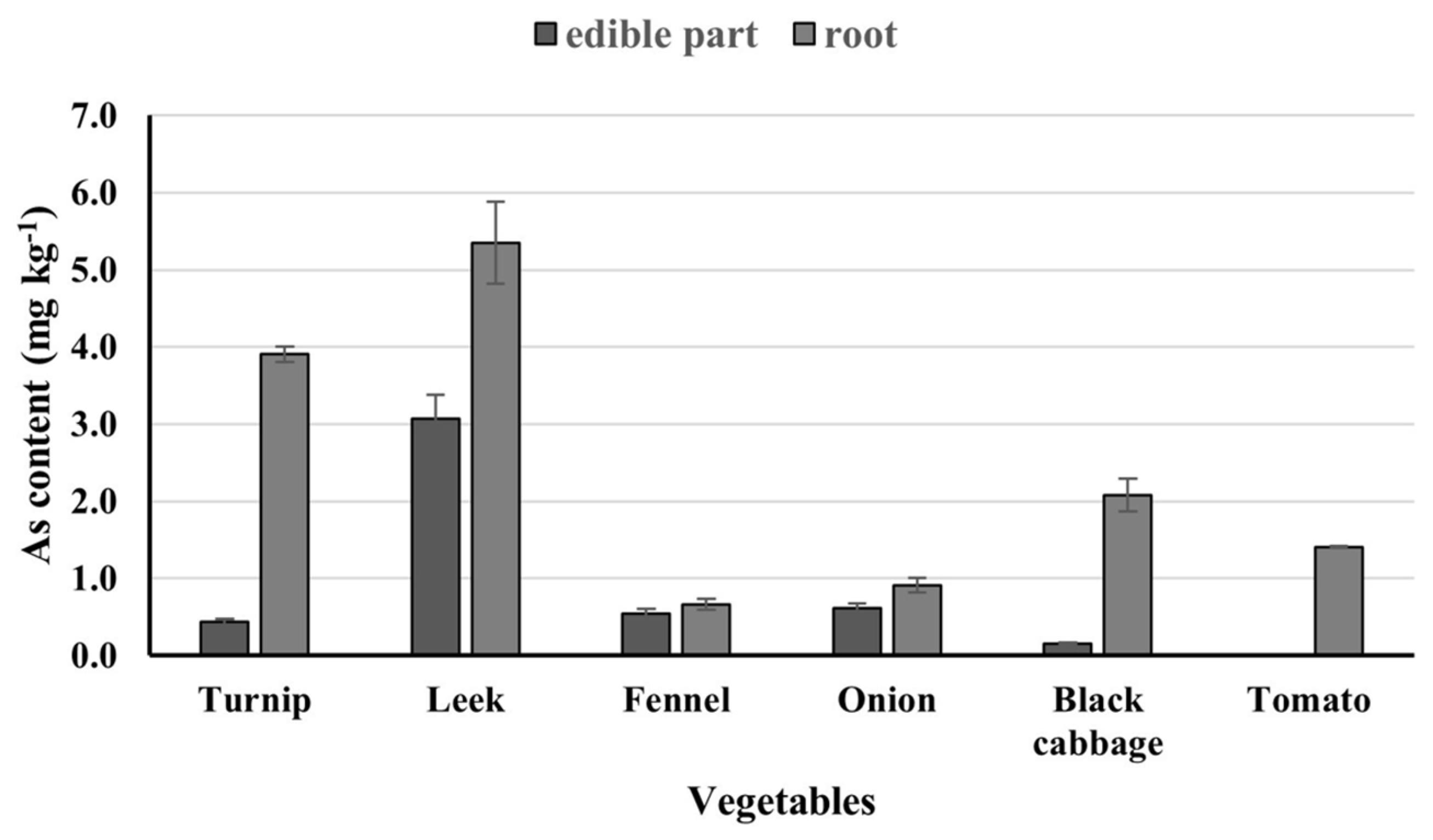
4.3. Soils and Vegetables

The statistical summary of all soil sampling surveys for the topsoil (0–20 cm) and the subsoil (80–100 cm) is reported in

Table 3. Statistical summary of soil sampling surveys (n = 63 for topsoil and n = 63 for deeper layer).

As (mg/kg)	Topsoil (0–20 cm)	Subsoil (80–100 cm)
Average	38.5	46.4
Median	26.5	26.9
Minimum	6.3	8.6
Maximum	200	211
Standard Error	4.4	3.7

.

The average value of As content in both topsoil and subsoil exceeded the threshold for the total As content (20 mg/kg) imposed by the Italian Regulations. The most contaminated areas are located in the upper part of the Baccatoio stream catchment and where the stream enters the alluvial plain [59]. Forty-nine percent of both topsoil and subsoil samples had As contents higher than 20 mg/kg, exceeding the threshold value.

In Figure 6, the average concentrations of As in the edible portions and roots of the different horticultural plants are reported. The values for the edible portions ranged from 0.2 to 3.1 mg/kg (on a dry weight basis). In the 2015 survey, arsenic was detected in the edible parts of leek (maximum concentration = 4.1 mg/kg), turnip (max = 1.3 mg/kg), fennel (max = 0.9 mg/kg), onion (max = 0.5 mg/kg) and black cabbage (max = 0.3 mg/kg), while it was not detected in tomato fruits. As expected, higher concentrations of As were found in the roots, which accumulate arsenic, translocating only small amounts into the edible components.

The averaged As concentrations measured in tomato fruits (spring/summer) and black cabbage leaves (autumn/winter) collected in 2017 are shown in Figure 7. The average arsenic concentration in tomato fruits was 0.18 mg/kg, with some higher concentration hotspots (up to 3.7 mg/kg) observed in the upper part of the Baccatoio stream catchment. Arsenic in the edible black cabbage leaves reached 0.4 mg/kg.

4.4. Risk Analysis

Health risk assessment, based on typical human exposure assessment assumptions and standard toxicological guidance values, was performed (

Table 4. Hazard Quotient (HQ) for non-carcinogenic and Risk (R) for carcinogenic effects calculated for different exposure routes, for children (defined as an individual between one and six years of age) and adult receptors (in brackets values for adults when different). Soil cumulative risks (HIi and Ri) and Risks from vegetables are also reported. Arsenic concentration values of 46.4, 0.18 and 0.4 mg/kg were used for soil, tomato and black cabbage, respectively. Carcinogenic effects for soil are represented by a single value because they were calculated using an age-adjusted factor (see text). SSL (surface soil) for each exposure route and their sums were calculated according to [56].

	Soil Ingestion	Dermal Contact	Inhalation Dust	HIi	Ri	Vegetables Ingestion (Tomato)	Vegetable Ingestion (Cabbage)	Sum of Soil Exposures
HQ *	1.19 (0.127)	0.166 (2.54 × 10−2)	2.05 × 10−5	1.36 (0.152)		2.92 (0.625)	0.213 (4.57 × 10−2)
R **	6.54 × 10−5	1.03 × 10−5	5.66 × 10−10		7.57 × 10−5	1.12 × 10−4 (9.64 × 10−5)	8.22 × 10−6 (7.05 × 10−6)
SSL	0.71	4.50	8.20 × 10−4					0.61

* RfD_oral = 3 × 10⁻⁴ (mg/kg/day); RfD_derm = RfD; RfC = 1.5 × 10⁻⁵ (mg/m³). ** SF_oral = 1.5 (mg/kg/day)⁻¹; SF_derm = SF_oral; IUR = 4.30 × 10⁻³ (μg/m³)⁻¹. Note: RfD_derm and SF_derm are assumed to be equal to RfD_oral and SF_oral, respectively, since it is not necessary to apply any “gastrointestinal absorption factor” to adjust available oral toxicity values [48,51].

) for the highest value of arsenic content (see Table 3). The risk derived from the consumption of tomatoes and black cabbage was also assessed. For non-carcinogenic effects, the obtained HI was higher than the acceptance threshold for children in a residential setting; the risk was generally unacceptable in the case of carcinogenic effects. The calculated individual soil screening levels (SSLs) are given in Table 4. It can be observed that the obtained screening values are significantly lower than the average As concentrations measured in soil. Furthermore, SSLs are significantly lower than the threshold imposed by Italian regulations for residential soil (20 mg/kg).

5. Discussion

5.1. Source and Fate of Arsenic Contamination

The main source of As contamination is geogenic. The weathering of the As-bearing mineral phases outcropping upstream the Baccatoio catchment, followed by erosion and transport during the evolution of the alluvial plain, may have a key role. In particular, fluctuations in the groundwater lever and/or the introduction of oxygenated recharge water through hydraulic connections may represent the hydrogeological control for the oxidative dissolution of spatially distributed lenses of sulfides, triggering As release and mobility in the aquifer systems under dynamic redox conditions ([60] and references therein). Indeed, As-bearing pyrite oxidation causes the concomitant release of Fe and S, and the fate of As is determined by the processes affecting the mineralogical characteristics of the aquifer media, in particular the precipitation of newly formed hydrous ferric oxides from supersaturated waters acting as As sorbents. In addition, the distribution of As in groundwater indicates that the most contaminated wells are located in the intermediate zone of the plain (Figure 8), characterized by sediments from a lacustrine/marshy environment including peats and peaty clays (Figure 4), suggesting the possibility that natural organic matter (NOM) in the aquifer assists As’s release and fate. Indeed, NOM serves as a geochemical trap for arsenic and may drive the dissolution of As-bearing iron oxyhydroxides in the aquifer sediments in a reducing environment, allowing the transformation of arsenate species to the more mobile arsenite. Along with oxidation, the As immobilized by NOM can be released and partly adsorbed on newly formed metastable iron oxyhydroxides, and the dissolution of As-hosting Fe hydroxides takes place when reducing conditions prevail. The complex scenario for As sequestration and release by high-iron sediments and organic matter not uniformly distributed in the aquifer, and the role of subsurface bacterial communities, results in the decoupling of As and Fe in groundwater.

It must also be noted that a hydraulic connection exists between the superficial aquifer horizons and the Baccatoio stream, especially in the upper and middle part of the alluvial fan. This is supported by field observations which indicate that, when it is minimally fed by springs, the Baccatoio stream loses water and almost vanishes, reducing the streamflow and recharging the aquifer, as expected in these geomorphological settings.

The Baccatoio stream waters are supersaturated with respect to a number of iron minerals, allowing yellowish and reddish precipitates to form and determining a high As concentration in bed-stream sediments [61]. When As-hosting iron oxyhydroxides become buried in the Baccatoio streambed sediments in the reducing conditions of the hyporheic zone, arsenic may be released via reductive dissolution. The hyporheic zone may hence act as an interface for As transport between the surface and the shallower groundwater in the stream-aquifer system, and As can subsequently infiltrate through the aquifer sediments. The possible evolution of a freshwater aquifer with the ionic constituents that characterize the Baccatoio stream water is supported by the hydrogeochemical pattern shown in the Piper diagram (Figure 5).

5.2. Soil, Vegetables and Risk Analysis

Arsenic is not an essential nutrient for plants and can reach toxicity levels in cases of high concentration in the soil [62]; the soil pH regulates its availability, speciation and fate in plants [63]. The sub-acidic conditions of the investigated soils, in addition to the relatively high As concentration, affects arsenic mobility, increasing the phytoavailability and uptake by plants. The background concentration of As in soil mainly depends on the lithology and type of soils, ranging from 5 to 10 mg/kg [64]. Several authors showed that As concentration in soils of polluted areas varied from 126 to 1600 mg/kg [64]. In our study, the soil samples of five horticultural gardens had As contents higher than 100 mg/kg.

Usually, the As concentration in plants is less than 1 mg/kg (dw) in uncontaminated soils; however, the As amount can increase up to 0.1 wt% in contaminated soils [65]. According to several authors, the threshold of 0.5 mg/kg can be considered as the maximum allowable limit [66]. In this case, the vegetables growing in the Baccatoio area should not be consumed since, for most vegetables, the edible parts exceed this limiting value.

According to the literature [67], vegetables like radish (turnip, leek, fennel, onion) that grow in contaminated soils accumulate higher amounts of As than leafy vegetables (black cabbage), as here observed. In addition, it can be inferred that plant metabolism plays an important role, and leafy vegetables (such as black cabbage) accumulate more arsenic than tomatoes.

Soil risk assessment indicates that the major threat for health associated with As is through ingestion. Dermal contact yields potential adverse health effects considering carcinogenic effects only; inhalation pathways do not produce any significant health risk. As regards vegetables, a carcinogenic risk exists for tomato and black cabbage ingestion. For non-carcinogenic effects, the chronic daily intake exceeds the reference dose for tomatoes in the case of children only.

The calculated SSLs reveal that the average As concentration measured in soil should be considered of potential toxicological concern. It is worth noting that the calculated SSL value is based on a target cancer risk of 10⁻⁶. Widely divergent cleanup targets, guidelines and standards for arsenic in soils have been established by many regulatory organizations. In addition, many countries use naturally occurring background or baseline soil arsenic levels as their screening guidance. It should also be considered that risk assessments carried out following international guidelines are often based on conservative assumptions and default exposure parameters, which represent a “reasonable maximum exposure” condition for long-term/chronic exposure. For example, in the case of the soil ingestion pathway, it is assumed that, for the whole period over which the outdoor exposure is averaged, the human target, child or adult, can accidentally ingest 200 and 100 mg of soil, respectively, every day. The SSL concentration values obtained in this study, intended as cautionary, are lower than the As concentration threshold in soil imposed by the current Italian regulations. This opens a question about the actual validity of regulatory threshold values for arsenic in soil and highlights the need for site-specific health risk assessments and to revise conservative assumptions before planning any remedial action.

6. Conclusions

In the Versilia Plain, the oxidation of As-bearing sulfides in the Baccatoio alluvial fan, possibly driven by a hydrogeological control, is supposed to be the main source of groundwater contamination. Arsenic release from the Baccatoio streambed sediments may also contribute to the shallower aquifer contamination through stream–aquifer interactions, possibly depending on flow regimes. The Baccatoio stream is also probably the main route for the spatial arsenic distribution in soils, in particular upstream, through water and bed-load transport. Arsenic-contaminated irrigation groundwater may also contribute to soil contamination. Arsenic uptake by edible plants occurs to different extents. Risk assessment indicates that arsenic may contribute to adverse health outcomes for humans by direct soil exposure routes and vegetable ingestion. In particular, the calculated soil screening level is significantly lower than the arsenic concentration measured in soil, and below the threshold limit imposed by Italian regulations. This raises concerns for both regulators and risk assessors and requires additional site-specific investigations.

A long-term systematic monitoring of contaminated wells is recommended in order to evaluate changes from season to season and from year to year, also in response to varying climatic conditions.

In addition, public awareness of groundwater safety is important for promoting household water treatment in order to prevent, or at least reduce, health impacts. Making groundwater exploitation from private wells illegal by local regulations represents a first action for disease prevention.

References

1. Abdul, K.S.M.; Jayasinghe, S.S.; Chandana, E.P.S.; Jayasumana, C.; De Silva, P.M.C.S. Arsenic and human health effects: A review. Enviroin. Toxicol. Pharmacol. 2015, 40, 828–846. [Google Scholar] [CrossRef] [PubMed]
2. Huhes, M.F.; Beck, B.D.; Chen, Y.; Lewis, A.S.; Thomas, D.J. Arsenic exposure and toxicology: A historical perspective. Toxicol. Sci. 2011, 123, 305–332. [Google Scholar] [CrossRef] [PubMed]
3. Hopenhayn, C. Arsenic in drinking water: Impact on human health. Elements 2006, 2, 103–107. [Google Scholar] [CrossRef]
4. Ravencroft, P.; Brammer, H.; Richards, K. Arsenic Pollution: A Global Synthesis; RGS-IBG Book Series; Wiley-Blackwell: Hoboken, NJ, USA, 2009; 616p. [Google Scholar]
5. Upadhyay, M.K.; Shukla, A.; Yadav, P.; Srivastava, S. A review of arsenic in crops, vegetables, animals and food products. Food Chem. 2019, 276, 608–618. [Google Scholar] [CrossRef]
6. Majumder, S.; Banik, P. Geographical variation of arsenic distribution in paddy soil, rice and rice-based products: A meta-analytic approach and implications to human health. J. Environ. Manag. 2019, 233, 184–199. [Google Scholar] [CrossRef]
7. WHO. Arsenic. In Guidelines for Drinking-Water Quality; World Health Organization: Geneva, Switzerland, 1993; Volume 1. [Google Scholar]
8. Smedley, P.L. Arsenic in groundwater. In Arsenic in Ground Water; Welch, A.H., Stollenwerk, K.G., Eds.; Geochemistry and Occurrence; Kluwer Academic Publishers: Boston, MA, USA; Dordrecht, The Netherlands; London, UK, 2003; pp. 179–209. [Google Scholar]
9. Charlet, L.; Polya, D.A. Arsenic in shallow, reducing groundwaters in southern Asia: An environmental health disaster. Elements 2006, 2, 91–96. [Google Scholar] [CrossRef]
10. Mukherjee, A.; Verma, S.; Gupta, S.; Henke, K.R.; Bhattacharya, P. Influence of tectonics, sedimentation and aqueous flow cycles on the origin of global groundwater arsenic: Paradigms from three continents. J. Hydrol. 2014, 518, 284–288. [Google Scholar] [CrossRef]
11. Jiang, J.-Q.; Ashekuzzaman, S.M.; Jiang, A.; Sharifuzzaman, S.M.; Chowdhury, S.R. Arsenic Contaminated Groundwater and Its Treatment Options in Bangladesh. Int. J. Environ. Res. Public Health 2013, 10, 18–46. [Google Scholar] [CrossRef]
12. Abbasnejad, A.; Mirzaie, A.; Derakhshani, R.; Esmaeilzadeh, E. Arsenic in groundwaters of the alluvial aquifer of Bardsir plain, SE Iran. Environ. Earth Sci. 2013, 69, 2549–2557. [Google Scholar] [CrossRef]
13. Webster, J.G.; Nordstrom, D.K. Geothermal arsenic. In Arsenic in Ground Water; Welch, A.H., Stollenwerk, K.G., Eds.; Geochemistry and Occurrence; Kluwer Academic Publishers: Boston, MA, USA; Dordrecht, The Netherlands; London, UK, 2003; pp. 101–125. [Google Scholar]
14. Bundschuh, J.; Maity, J.P. Geothermal arsenic: Occurrence, mobility and environmental implications. Renew. Sustain. Energy Rev. 2015, 42, 1214–1222. [Google Scholar] [CrossRef]
15. Ortega-Guerrero, A. Evaporative concentration of arsenic in groundwater: Health and environmental implications, La Laguna Region, Mexico. Environ. Geochem. Health 2017, 39, 987–1003. [Google Scholar] [CrossRef] [PubMed]
16. Ishiguro, S. Industries using arsenic and arsenic compounds. Appl. Organomet. Chem. 1992, 6, 323–331. [Google Scholar] [CrossRef]
17. Han, F.X.; Su, Y.; Monts, D.L.; Plodinec, M.J.; Banin, A.; Triplett, G.E. Assessment of global industrial-age anthropogenic arsenic contamination. Naturwissenschaften 2003, 90, 395–401. [Google Scholar] [CrossRef] [PubMed]
18. Carbonell-Barrachina, A.A.; Signes-Pastor, A.J.; Vázquez-Araújo, L.; Sengupta, B. Presence of arsenic in agricultural products from arsenic-endemic areas and strategies to reduce arsenic intake in rural villages. Mol. Nutr. Food Res. 2009, 53, 531–541. [Google Scholar] [CrossRef] [PubMed]
19. Abad-Valle, P.; Álvarez-Ayuso, E.; Murciego, A.; Muñoz-Centeno, L.M.; Alonso-Rojo, P.; Villar-Alonso, P. Arsenic distribution in a pasture area impacted by past mining activities. Ecotoxicol. Environ. Saf. 2018, 147, 228–237. [Google Scholar] [CrossRef]
20. Wongsasuluk, P.; Tun, A.Z.; Chotpantarat, S.; Siriwong, W. Related health risk assessment of exposure to arsenic in some heavy metals in gold mines in Banmauk Township, Myanmar. Sci. Rep. 2021, 11, 22843. [Google Scholar] [CrossRef]
21. Park, J.H.; Han, Y.-S.; Ahn, J.S. Comparison of arsenic co-precipitation and adsorption by iron minerals and the mechanism of arsenic natural attenuation in a mine stream. Water Res. 2016, 106, 295–303. [Google Scholar] [CrossRef] [PubMed]
22. Lewińska, K.; Duczmal-Czernikiewicz, A.; Karczewska, A.; Dradrach, A.; Iqbal, M. Arsenic forms in soils of various settings in the historical ore mining and processing site of Radzimowice, Western Sudetes. Minerals 2021, 11, 491. [Google Scholar] [CrossRef]
23. Panagiotaras, D.; Nikolopoulos, D. Arsenic occurrence and fate in the environment; a geochemical perspective. J. Earth Sci. Clim. Chang. 2015, 6, 269. [Google Scholar]
24. Barral-Fraga, L.; Barral, M.T.; MacNeill, K.L.; Martiñá-Prieto, D.; Morin, S.; Rodríguez-Castro, M.C.; Tuulaikhuu, B.-A.; Guash, H. Biotic and abiotic factors influencing arsenic biogeochemistry and toxicity in fluvial ecosystems: A review. Int. J. Environ. Res. Public Health 2020, 17, 2331. [Google Scholar] [CrossRef]
25. Smedley, P.L.; Kinniburgh, D.G. A review of the source, behavior and distribution of arsenic in natural waters. Appl. Geochem. 2002, 17, 517–568. [Google Scholar] [CrossRef]
26. Taylor, V.; Goodale, B.; Raab, A.; Schwerdtle, T.; Reimer, K.; Conklin, S.; Karagas, M.; Francesconi, K. Human exposure to organic arsenic species from seafood. Sci. Total Environ. 2017, 580, 266–282. [Google Scholar] [CrossRef] [PubMed]
27. Dzombak, D.A.; Morel, F.M.M. Surface Complexation Modeling: Hydrous Ferric Oxide; Wiley and Sons: New York, NY, USA, 1990; 393p. [Google Scholar]
28. Stollenwerk, K.G. Geochemical processes controlling transport of arsenic in groundwater: A review of adsorption. In Arsenic in Ground Water; Welch, A.H., Stollenwerk, K.G., Eds.; Geochemistry and Occurrence; Kluwer Academic Publishers: Boston, MA, USA; Dordrecht, The Netherlands; London, UK, 2003; pp. 67–100. [Google Scholar]
29. Root, R.A.; Dixit, S.; Campbell, K.M.; Jew, A.D.; Hering, J.G.; O’Day, P.A. Arsenic sequestration by sorption processes in high-iron sediments. Geochim. Cosmochim. Acta 2007, 71, 5782–5803. [Google Scholar] [CrossRef]
30. Schacht, L.; Ginder-Vogel, M. Arsenite depletion by manganese oxides: A case study on the limitations of observed first order rate constants. Soil Syst. 2018, 2, 39. [Google Scholar] [CrossRef]
31. Jain, A.; Loeppert, R.H. Effects of competing anions on the adsorption or arsenate and arsenite by ferrihydrite. J. Environ. Qual. 2000, 9, 1422–1430. [Google Scholar] [CrossRef]
32. Wang, S.; Mulligan, C.N. Effects of natural organic matter on arsenic release from soils and sediments into groundwater. Environ. Geochem. Health 2006, 28, 197–214. [Google Scholar] [CrossRef]
33. Williams, P.N.; Zhang, H.; Davison, W.; Meharg, W.D.; Hossain, M.; Norton, G.J.; Brammer, H.; Islam, M.R. Organic matter- solid phase interactions are critical for predicting arsenic release and plant uptake in Bangladesh paddy soils. Environ. Sci. Technol. 2011, 45, 6080–6087. [Google Scholar] [CrossRef]
34. Langner, P.; Mikutta, C.; Kretzschmar, R. Arsenic sequestration by organic sulphur in peat. Nat. Geosci. 2012, 5, 66–73. [Google Scholar] [CrossRef]
35. Li, N.; Wang, J.; Song, W.-Y. Arsenic uptake and translocation in plants. Plant Cell Physiol. 2016, 57, 4–13. [Google Scholar] [CrossRef]
36. Meena, M.K.; Singh, A.K.; Prasad, L.K.; Islam, A.; Meena, M.D.; Dotaniya, M.L.; Singh, H.; Yadav, B.L. Impact of arsenic-polluted groundwater on soil and produce quality: A food chain study. Environ. Monit. Assess. 2020, 192, 785. [Google Scholar] [CrossRef]
37. Luppichini, M.; Noti, V.; Pavone, D.; Bonato, M.; Ghizzani Marcìa, F.; Genovesi, S.; Lemmi, F.; Rosselli, L.; Chiarenza, N.; Colombo, M.; et al. Web mapping and real–virtual itineraries to promote feasible archaeological and environmental tourism in Versilia (Italy). ISPRS Int. J. Geo-Inform. 2022, 11, 460. [Google Scholar] [CrossRef]
38. Carmignani, L.; Giglia, G.; Kligfield, R. Structural evolution of the Apuan Alps: An example of continental margin deformation in the northern Apennines, Italy. J. Geol. 1978, 86, 487–504. [Google Scholar] [CrossRef]
39. Piccini, L.; Nannoni, A.; Poggetti, E. Hydrodynamics of karst aquifers in metamorphic carbonate rocks: Results from spring monitoring in the Apuan Alps (Tuscany, Italy). Hydrogeol. J. 2023, 31, 241–255. [Google Scholar] [CrossRef]
40. Lattanzi, P.; Benvenuti, M.; Costagliola, P.; Tanelli, G. An overview on recent research on the metallogeny of Tuscany, with special reference to Apuane Alps. Mem. Soc. Geol. It. 1994, 48, 613–625. [Google Scholar]
41. D’Orazio, M.; Biagioni, C.; Dini, A.; Vezzoni, S. Thallium-rich pyrite ores from Apuan Alps, Tuscany, Italy: Constraints for their origin and environmental concerns. Miner. Deposita 2017, 52, 687–707. [Google Scholar] [CrossRef]
42. Perotti, M.; Petrini, R.; D’Orazio, M.; Ghezzi, L.; Giannecchini, R.; Vezzoni, S. Thallium and other potentially toxic elements in the Baccatoio Stream catchment (northern Tuscany, Italy) receiving drainages from abandoned mines. Mine Water Environ. 2018, 37, 431–441. [Google Scholar] [CrossRef]
43. Campanella, B.; Onor, M.; D’Ulivo, A.; Giannecchini, R.; D’Orazio, M.; Petrini, R.; Bramanti, E. Human exposure to thallium through tap water: A study from Valdicastello Carducci and Pietrasanta (northern Tuscany, Italy). Sci. Total Environ. 2015, 548–549, 33–42. [Google Scholar] [CrossRef]
44. Ghezzi, L.; D’Orazio, M.; Doveri, M.; Lelli, M.; Petrini, R.; Giannecchini, R. Groundwater and potentially toxic elements in a dismissed mining area: Thallium contamination of drinking spring water in the Apuan Alps (Tuscany, Italy). J. Geoch. Expl. 2019, 197, 84–92. [Google Scholar] [CrossRef]
45. Antisari, L.V.; Bianchini, G.; Dinelli, E.; Falsone, G.; Gardini, A.; Simoni, A.; Tassinari, R.; Vianello, G. Critical evaluation of an intercalibration project focused on the definition of new multi-element soil reference materials (AMS-MO1 and AMS-ML1), EQA. EQA Int. J. Environ. Qual. 2014, 15, 41–64. [Google Scholar]
46. Report E 2081-00; Standard Provisional Guide for Risk-Based Corrective Action. American Society for Testing Materials (ASTM): West Conshohocken, PA, USA, 2000.
47. US EPA. Soil Screening Guidance: Technical Background Document; EPA/540/R-95/128; US Environmental Protection Agency, Office of Emergency and Remedial Response: Washington, DC, USA, 1996.
48. US EPA. Supplemental Guidance for Developing Soil Screening Levels for Superfund Sites; OSWER 9355.4-24; US Environmental Protection Agency, Office of Emergency and Remedial Response: Washington, DC, USA, 2002.
49. US EPA. Risk Assessment; US Environmental Protection Agency: Washington, DC, USA, 2022. Available online: https://www.epa.gov/risk (accessed on 27 March 2023).
50. US EPA. Human Health Evaluation Manual, Supplemental Guidance: Update of Standard Default Exposure Factors; OSWER 9200.1-120; US Environmental Protection Agency, Office of Solid Waste and Emergency Response: Washington, DC, USA, 2014.
51. US EPA. Regional Screening Level (RSLs)—Generic Tables; US Environmental Protection Agency: Washington, DC, USA, 2022. Available online: https://www.epa.gov/risk/regional-screening-levels-rsls-generic-tables (accessed on 27 March 2023).
52. Leclercq, C.; Arcella, D.; Piccinelli, R.; Sette, S.; Le Donne, C.; Turrini, A. The Italian National Food Consumption Survey INRAN-SCAI 2005-06: Main results in terms of food consumption. Public Health Nutr. 2009, 12, 2504–2532. [Google Scholar] [CrossRef]
53. US EPA. Risk Assessment Guidance for Superfund. Volume I. Human Health Evaluation Manual, Supplemental Guidance: Standard Default Exposure Factors; EPA/540/1-89/002; US Environmental Protection Agency, Office of Emergency and Remediation Response: Washington, DC, USA, 1989.
54. US EPA. Risk Assessment Guidance for Superfund—Volume I: Human Health Evaluation Manual (Part F, Supplemental Guidance for Inhalation Risk Assessment); U.S.EPA-540-R-070-002; Office of Superfund Remediation and Technology Innovation, US Environmental Protection Agency: Washington, DC, USA, 2009.
55. Ghezzi, L.; Arrighi, S.; Giannecchini, R.; Bini, M.; Valerio, M.; Petrini, R. The Legacy of Mercury Contamination from a Past Leather Manufacturer and Health Risk Assessment in an Urban Area (Pisa Municipality, Italy). Sustainability 2022, 14, 4367. [Google Scholar] [CrossRef]
56. US EPA. Regional Screening Level (RSLs)—Equations; US Environmental Protection Agency: Washington, DC, USA, 2022. Available online: https://www.epa.gov/risk/regional-screening-levels-rsls-equations#res (accessed on 27 March 2023).
57. US EPA. Risk Assessment Guidance for Superfund. Volume I. Human Health Evaluation Manual, Part B; EPA/540/R-92/003; US Environmental Protection Agency, Office of Emergency and Remedial Response: Washington, DC, USA, 1991.
58. Baroni, C.; Pieruccini, P.; Bini, M.; Coltorti, M.; Fantozzi, P.L.; Guidobaldi, G.; Nannini, D.; Ribolini, A.; Salvatore, M.C. Geomorphological and neotectonic map of the Apuan Alps (Tuscany, Italy). Geogr. Fis. Din. Quat. 2015, 38, 201–227. [Google Scholar]
59. Vittori Antisari, L.; Bini, C.; Ferronato, C.; Gherardi, M.; Vianello, G. Translocation of potential toxic elements from soil to black cabbage (Brassica oleracea L.) growing in an abandoned mining district area of the Apuan Alps (Tuscany, Italy). Environ. Geochem. Health 2020, 42, 2413–2423. [Google Scholar] [CrossRef] [PubMed]
60. Battistel, M.; Stolze, L.; Muniruzzaman, M.; Rolle, M. Arsenic release and transport during oxidative dissolution of spatially distributed sulfide minerals. J. Hazard. Mat. 2021, 409, 124651. [Google Scholar] [CrossRef] [PubMed]
61. Ghezzi, L.; Buccianti, A.; Giannecchini, R.; Guidi, M.; Petrini, R. Geochemistry of mine stream sediments and the contro, of potentially toxic element migration: A case study from the Baccatoio basin (Tuscany, Italy). Mine Water Environ. 2021, 40, 722–735. [Google Scholar]
62. Finnegan, P.M.; Chen, W. Arsenic Toxicity: The Effects on Plant Metabolism. Front. Physiol. 2012, 3, 182. [Google Scholar] [CrossRef]
63. Khalid, S.; Shahid, M.; Niazi, N.K.; Rafiq, M.; Bakhat, H.F.; Imran, M.; Abbas, T.; Bibi, I.; Dumat, C. Arsenic behaviour in soil-plant system: Biogeochemical reactions and chemical speciation influences. In Enhancing Cleanup of Environmental Pollutants; Springer: Berlin/Heidelberg, Germany, 2017; pp. 97–140. [Google Scholar]
64. Patel, K.S.; Pandey, P.K.; Martín-Ramos, P.; Corns, W.T.; Varol, S.; Bhattacharyaf, P.; Zhu, Y. A review on arsenic in the environment: Contamination, mobility, sources, and exposure. RSC Adv. 2023, 13, 8803. [Google Scholar] [CrossRef]
65. Austruy, A.; Wanat, N.; Moussard, C.; Vernay, P.; Joussein, E.; Ledoigt, G.; Hitmi, A. Physiological impacts of soil pollution and arsenic uptake in three plant species: Agrostis capillaris, Solanum nigrum and Vicia faba. Ecotoxicol. Environ. Saf. 2013, 90, 28–34. [Google Scholar] [CrossRef] [PubMed]
66. Natasha; Shahid, M.; Khalid, S.; Niazi, N.K.; Murtaza, B.; Ahmad, N.; Farooq, A.; Zakir, A.; Imran, M.; Abbas, G. Health risks of arsenic build-up in soil and food crops after wastewater irrigation. Sci. Tot. Environ. 2021, 772, 145266. [Google Scholar] [CrossRef]
67. Spognardi, S.; Bravo, I.; Beni, C.; Menegoni, P.; Pietrelli, L.; Papetti, P. Arsenic accumulation in edible vegetables and health risk reduction by groundwater treatment using an adsorption process. Environ. Sci. Pollut. Res. 2019, 26, 32505–32516. [Google Scholar] [CrossRef]
Figure 1. Location of the study area (in red). The yellow dashed line represents the upper part of the Baccatoio stream catchment.
Applsci 13 05446 g001
Figure 2. Groundwater (red dots), soil and vegetable (yellow dots) sampling stations.
Applsci 13 05446 g002
Figure 3. Geological sketch map of the study area. The section tracks are also shown (see Discussion) (1: beach ridge; 2: marsh area; 3: alluvial fan (mixed grain size); 4 alluvial fan (mainly silty grain size); 5: alluvial fan (sandy grain size); 6: alluvial fan (gravelly grain size): 7 current beach; 8: Apuan hills (bedrock); 9: boreholes (from Geological Map of Tuscany, 1:50,000 scale)).
Applsci 13 05446 g003
Figure 4. Hydrostratigraphic cross-section A-A′ and B-B′ (section tracks in Figure 3) (the vertical scale is exaggerated compared with the horizontal scale). The black lines represent boreholes; the red lines indicate the wells in which the highest As concentrations were found.
Applsci 13 05446 g004
Figure 5. Piper diagram for the studied groundwater (black circles), indicating the different prevailing hydrofacies with Ca-HCO3 type. The water chemistry of Baccatoio stream water is superimposed (red triangles) (Data source: [42]).
Applsci 13 05446 g005
Figure 6. Average As content in different vegetables, divided into edible parts (dark gray) and roots (light gray), during the first (2015) survey. The error bars were calculated as standard error.
Applsci 13 05446 g006
Figure 7. Averaged As content determined in fruits and roots and leaves and roots for tomato and black cabbage, respectively, during the second (2017) survey. The error bars were calculated as standard error.
Applsci 13 05446 g007
Figure 8. Distribution of arsenic concentration in groundwater.
Applsci 13 05446 g008