Geometric Analysis of Sun-Assisted Lunar Transfer Trajectories in the Planar Bicircular Four-Body Model

Abstract

This research presents a geometric analysis of Sun-assisted low-energy lunar transfers and several convenient tools that enable the systematic trajectory design in the framework of the planar bicircular restricted four-body problem. By analogy with the patched conic approximation approach for high-energy transfers, a Sun-assisted low-energy trajectory is divided into three legs. Two interior legs, departing and arriving, are located inside the Earth–Moon region of prevalence and designed in the Earth–Moon circular restricted three-body problem, whereas the exterior leg lies outside the region of prevalence and is calculated in the Earth–Moon–Sun bicircular restricted four-body model. The whole trajectory is obtained by smoothly patching the three legs on the boundary of the region of prevalence. The arrival conditions are met by targeting a specific point in the L₂ lunar gateway. The interior legs are easily adjustable to the four-body dynamics. The database of planar lunar transfer trajectories can be used to select an initial guess for the multiple-shooting procedure of designing a three-dimensional Sun-assisted lunar transfer in high-fidelity dynamical models.

1. Introduction

The Moon and its vicinity are of great interest for both science and space exploration. In recent years, the world’s major space agencies have been jointly involved in the research and development of a habitable lunar orbital station named the Lunar Orbital Platform-Gateway (LOP-G) [1]. The station is planned to be used as a communication hub, a science laboratory, a short-term habitation module, and a holding area for rovers and other robotic vehicles. The design of fuel-efficient transfers between a low-Earth parking orbit and the near-lunar space is one of the cornerstones for the rapid development of lunar infrastructure.

The first steps in the research of lunar transfer’s feasibility and characteristics have been made by the Soviet scientist Vsevolod Egorov in the early 1950s. His Ph.D. thesis contains the fundamental results about direct flights to the Moon: Egorov was the first who answered the questions on the minimum initial speed for a spacecraft to reach the Moon, the existence and basic properties of free-return trajectories, and the sensitivity of a lunar transfer trajectory to initial conditions [2]. Egorov’s results played a crucial role in the first lunar missions. Sample trajectories to the Moon, distinguished by a short time of flight (several days) and hyperbolic arrival velocities, were designed by the patched conic approximation method; they require a significant cost to insert a spacecraft into a desired orbit around the Moon and are thus called high-energy trajectories.

When we replace the patched conic approximation with the circular restricted three-body problem (CR3BP), more efficient transfer trajectories—low-energy trajectories—emerge. The smart use of gravity of the primary and secondary celestial bodies enables considerable fuel savings compared to conventional high-energy transfer trajectories with translunar injection (TLI) and lunar orbit insertion (LOI) impulsive maneuvers. The price for such efficiency is an appreciably increased time of flight: a low-energy transfer takes months instead of days.

The first example of a low-energy Earth–Moon transfer trajectory was given by Charles Conley in 1968 [3]. He rigorously proved the existence of such trajectories and revealed their important feature of ballistic capture when no insertion maneuver is required for a spacecraft to be captured by the Moon’s gravity. The Keplerian energy (with respect to the Moon) is no longer the first integral in the CR3BP and naturally changes its sign from positive to negative as the spacecraft approaches the near-Moon region. One may distinguish interior and exterior ballistic capture, depending on from which libration point neck, L₁ or L₂, the spacecraft dives into the Moon’s Hill sphere. The former effect has been successfully leveraged in 2003 in the celebrated SMART-1 low-thrust mission [4]. The latter effect was demonstrated even earlier, in 1990, when Belbruno and Miller designed a rescue trajectory with exterior capture for the Japanese Hiten mission [5] (the very term of ballistic capture seems to be coined by Belbruno in the late 1980s). In the following paper [6], the same authors investigated the role of the Sun’s gravity perturbation more deeply, raising the perigee of a transfer trajectory. Ivashkin compared such a perturbing effect with the second impulse in a classic three-impulse bielliptic transfer. He deduced some analytical estimates useful for a better understanding of the mechanism of capture in the Earth–Moon–Sun system [7].

Following Conley’s ideas, a number of researchers have developed numerical methods of low-energy trajectory design based on the dynamical systems theory. Belbruno, who gave in [6] the initial algorithmic definition of a weak stability boundary (WSB) as a boundary of the region in the configuration space where the orbital motion around one of the celestial bodies is stable, later formalized this concept: the weak stability boundary of a given body is a set in the phase space that is located in the intersection of a certain Jacobi integral manifold and the region bounded by the hypersurface of zero Keplerian energy [8,9]. In contrast to capture by executing an LOI maneuver, ballistic capture is temporary. It is also referred to as weak.

To design a low-energy transfer trajectory in the three-body (Earth–Moon) or four-body (Earth–Moon–Sun) system, many numerical techniques have been developed that are based on searching for heteroclinic connections between the invariant manifolds of (quasi)periodic orbits around the L₁ and/or L₂ libration points [10,11,12,13]. In the planar CR3BP, using the tools of Poincaré and Keplerian maps, researchers have revealed the chaotic nature of the ballistic capture phenomenon and its intrinsic link with both the WSB and resonant orbits. Moreover, the resonance hopping theory has been developed [8,9,14,15,16,17]; convincing evidence has been discovered that there exists a close connection between the WSB set and invariant manifolds of libration point orbits [18,19].

When aerospace engineers refer to a WSB trajectory, they mean a Hiten-like low-energy trajectory starting from near-Earth orbit and exploiting the solar gravitational perturbation to ensure exterior ballistic capture by the Moon. Such a trajectory was utilized in NASA’s GRAIL mission in the period 2011–2012 [20] and, more recently, in the missions of CAPSTONE [21] and Danuri [22]. Depending on the final lunar orbit, a transfer trajectory may or may not include a large LOI impulse. In the latter case, a transfer can be reasonably called ballistic, though the term of ballistic lunar transfer (BLT) is often applied to any trajectory of this sort, no matter the magnitude of the required LOI impulse. Moreover, in our opinion, neither the name WSB nor BLT reflects the gravity of the Sun’s effect, the key feature of such transfer trajectories that singles them out from other low-energy transfers. So, we would like to coin the term of Sun-assisted lunar transfer (SALT). A SALT trajectory may be viewed as a special case of the broader class of WSB trajectories (for example, it is natural to consider SMART-like transfer trajectories to be included in the WSB class as well). SALT trajectories can be ballistic or thrust-augmented, as in the cases of recently launched Lunar IceCube [23] and EQUULEUS [24] missions.

The simplest dynamical model capturing the crucial Sun’s gravity perturbation effect is the bicircular restricted four-body problem (BR4BP), an extension of CR3BP where the Sun is also assumed to revolve in a distant circular orbit around the Earth–Moon barycenter. As the extensive global search for optimal two-impulse transfers in the planar BR4BP model clearly demonstrates, it is SALT trajectories that achieve the maximum fuel efficiency, especially if an intermediate lunar flyby is employed [25,26,27]. Intensive research on the development and application of SALT design techniques is now actively ongoing, primarily with periodic and quasiperiodic lunar libration point orbits as a transfer destination [28,29,30,31,32,33,34].

To this moment, all the existing techniques of designing a SALT trajectory rely on direct numerical optimization procedures. When possible, the invariant manifold geometry can be employed (e.g., by using the Poincaré periapsis map) to obtain a good initial guess for such a procedure. The major obstacle to the regular convergence of the procedure from some initial guess is due to the fact that the initial and final legs of a lunar transfer trajectory obey the fast near-Earth/near-Moon dynamics, which causes extreme sensitivity to boundary conditions. The same issue for high-energy trajectories was successfully resolved with the patched conic approximation that decouples the design of a sensitive trajectory leg in the close vicinity of a flyby body. The aim of this research is to develop a similar methodology and, by applying it, to perform the analysis and classification of SALT trajectories. Leveraging the concept of the Earth–Moon region of prevalence, we assemble a SALT trajectory from the three legs: departing and arriving, designed in the Earth–Moon CR3BP, and the exterior leg, calculated in the Sun–Earth CR3BP or directly in the Earth–Moon–Sun BR4BP.

The structure of the paper is as follows. First, we outline the CR3BP and BR4BP models, together with the patched three-body approximation of the four-body dynamics. After that, the procedure of planar SALT trajectory design is described in detail. All three trajectory legs are separately examined. Along the way, we also analytically prove the quadrant rule, a well-known property of Sun-assisted lunar transfers. The geometric analysis of the designed SALT trajectories is conducted, and the distinct patterns are revealed that can help to select a good initial guess when designing a SALT trajectory in complex dynamical models.

2. Dynamical Models

Let us first introduce the dynamical models utilized in this study: the circular restricted three-body problem, the bicircular four-body problem, and the patched three-body model.

2.1. Circular Restricted Three-Body Problem

The circular restricted three-body problem model describes the orbital motion of a body of negligible mass (e.g., the spacecraft) in the gravitational field of two primaries (in our case, the Earth and the Moon) revolving with a constant angular velocity in circular orbits around their center of mass C. We denote by m_E and m_M the masses of the major primary (the Earth) and the minor primary (the Moon), respectively. The CR3BP equations of motion are usually written in the rotating reference frame with the origin at C: the x-axis connects the primaries and points toward the minor primary, the z-axis is directed along the angular momentum of the primaries, and the y-axis completes the right-handed system (Figure 1).

In the CR3BP, it is convenient to use a dimensionless system of units: the masses of the bodies are normalized so that $m_E=1-\mu$ and $m_M=\mu$, where $\mu =m_M/(m_E+m_M)$ is the CR3BP mass parameter, the angular velocity of the rotating frame is normalized to one, and the distance between m_E and m_M is normalized to 1. The dimensionless gravitational constant G is also identically equal to 1. For the Earth–Moon system, the corresponding units of distance, velocity and time are adopted as follows:

$$\begin{array}{cc}\hfill \mathrm{DU}& =384402\mathrm{km},\hfill \\ \hfill \mathrm{VU}& =1.0245441823\mathrm{km}/\mathrm{s},\hfill \\ \hfill \mathrm{TU}& =4.3425137728\mathrm{days},\hfill \end{array}$$

(1)

and the CR3BP mass parameter $\mu =0.0121505845$. In this system of units, the two primaries are at fixed positions $[-\mu ,0,0]$ and $[1-\mu ,0,0]$ along the x-axis. The equations of spacecraft motion are written in the nondimensional form as

$$\begin{array}{cc}\hfill \ddot{x}-2\dot{y}& =\frac{\partial {\mathsf{\Omega }}_3}{\partial x},\hfill \\ \hfill \ddot{y}+2\dot{x}& =\frac{\partial {\mathsf{\Omega }}_3}{\partial y},\hfill \\ \hfill \ddot{z}& =\frac{\partial {\mathsf{\Omega }}_3}{\partial z},\hfill \end{array}$$

(2)

where

$${\mathsf{\Omega }}_3(x,y,z)=\frac{x^2+y^2}{2}+\frac{1-\mu }{r_1}+\frac{\mu }{r_2}+\frac{\mu (1-\mu )}{2}$$

(3)

is the effective potential. The distances $r_1$ and $r_2$ from the spacecraft to $m_E$ and $m_M$ can be expressed by the formulas $r_1^2={(x+\mu )}^2+y^2+z^2$, $r_2^2={(x-1+\mu )}^2+y^2+z^2$.

It is well known that the CR3BP system (2) has an energy integral of motion, the Jacobi integral

$$J(x,y,z,\dot{x},\dot{y},\dot{z})=2{\mathsf{\Omega }}_3(x,y,z)-({\dot{x}}^2+{\dot{y}}^2+{\dot{z}}^2).$$

(4)

As a result, every CR3BP solution in the 6D phase space belongs to the 5D integral manifold $\mathcal{J}=\{[x,y,z,\dot{x},\dot{y},\dot{z}]\in {\mathbb{R}}^6|J(x,y,z,\dot{x},\dot{y},\dot{z})=\tilde{J}\}$ of level $\tilde{J}$. The planar motion is reproduced by setting $z\equiv 0$. Each planar solution lies on a three-dimensional Jacobi integral manifold in the four-dimensional phase space of the planar CR3BP.

2.2. Bicircular Restricted Four-Body Problem

The bicircular restricted four-body problem extends the Earth–Moon circular restricted three-body problem by incorporating the Sun’s gravitational perturbation. In the framework of the BR4BP model, the Sun is assumed to revolve in a circular orbit of radius $L\gg 1$ around the Earth–Moon center of mass in the same plane as the Moon does. The direction to the Sun in the CR3BP rotating reference frame is determined by ${\theta }_S$—the phase of the Sun (Figure 2).

The equations of spacecraft motion in the BR4BP model have the same nondimensional form as in the CR3BP if we modify the effective potential by adding

$${\mathsf{\Omega }}_S(x,y,z,t)=\frac{G{m}_S}{r_3\left(t\right)}-\frac{G{m}_S}{L^2}(xcos{\theta }_S\left(t\right)+ysin{\theta }_S\left(t\right)),$$

(5)

where $G{m}_S=3.289005596145305\times {10}^5$ is the dimensionless Sun’s gravitational parameter,

$$r_3\left(t\right)=\sqrt{{(x-Lcos{\theta }_S\left(t\right))}^2+{(y-Lsin{\theta }_S\left(t\right))}^2+z^2}$$

(6)

is the distance from the spacecraft to the Sun. The phase of the Sun grows linearly over time: ${\theta }_S\left(t\right)={\theta }_0+{\omega }_S(t-t_0)$. For $L=389.17$, which approximately corresponds to the ratio of the Sun–Earth and Earth–Moon distances, the rotation rate of the Sun is determined as follows:

$${\omega }_S=\sqrt{\frac{1+m_S}{L^3}}-1\approx -0.9253.$$

(7)

By analogy with the CR3BP, the planar case is derived by setting $z\equiv 0$.

2.3. Patched Three-Body Approximation

The BR4BP is among the simplest suitable models to design SALT trajectories, but it can be further simplified while still capturing the key dynamical effect of the Sun’s gravity. The idea behind such a simplification is very similar to the patched conic approximation approach for high-energy trajectories: the configuration space close to a planet and/or a moon is encircled by the region of prevalence (RoP) of this planet–moon three-body system. The dynamics in the RoP interior are well described by the planet–moon CR3BP model, whereas outside the RoP, the BR4BP or the Sun–planet CR3BP model is applied (in case of the Earth and the Moon, their barycenter usually performs the role of the minor primary).

The concept of the region of prevalence was first coined by Castelli [35] who defined the Earth–Moon region of prevalence as a region in the configuration space bounded by a closed curve of points where the error introduced in the right-hand sides of the equations of motion would be the same independently of which body we neglect in the Earth–Moon–Sun system, the Moon or the Sun. The region of prevalence is time-dependent: it is parameterized by the Sun’s phase ${\theta }_S$. The Earth–Moon RoP boundaries projected onto the $xy$-plane are shown for different solar phases by colored closed curves (Figure 3). To avoid time dependency, we define the mean-square averaged region of prevalence: its stationary boundary is chosen to have a simple elliptical form (the bold orange curve in Figure 3), with the principal axes parallel to the coordinate axes of the Earth–Moon rotating reference frame. In the dimensionless system of units specified by Equation (1), the points of this boundary in the $xy$-plane satisfy the equation

$$\frac{{(x+c)}^2}{a^2}+\frac{y^2}{b^2}=1,$$

(8)

where $a=1.44$, $b=1.05$, $c=-0.25$. Further in the paper, the area with the boundary given by Equation (8) is referred to simply as the Earth–Moon region of prevalence.

3. Synthesis and Analysis of Planar SALT Trajectories

To design a SALT trajectory, the four-body dynamics should be considered. However, when the spacecraft just departs the Earth or approaches the Moon, the Sun’s gravity can be neglected and the Earth–Moon CR3BP describes the dynamics accurately enough. Therefore, it seems reasonable to divide any SALT trajectory into three legs: the departing and arriving legs inside the Earth–Moon region of prevalence (thus, designed in the Earth–Moon CR3BP) and the exterior leg outside the RoP connecting the two interior legs. It is this leg that should reflect the effect of the Sun’s gravity pull.

The most comprehensive analysis of the SALT trajectory design problem can be done in the planar case where useful geometrical instruments are available, but before proceeding to this analysis, let us prove one general result known as the quadrant rule.

3.1. The Quadrant Rule

Researchers numerically designing Sun-assisted low-energy transfers are familiar with the property that the apogee of a SALT trajectory is located in either the second or the fourth quadrant of the Sun–Earth rotating reference frame centered at the Earth, as shown in Figure 4. Below, we explain this feature analytically.

In the patched three-body approximation, the perturbation due to the Sun’s gravity can be estimated by analyzing the increment of the Jacobi integral of the Earth–Moon three-body system along the exterior leg of a trajectory. Differentiating (4) in the BR4BP dynamics gives

$$\frac{dJ}{dt}=2\left(\frac{\partial {\mathsf{\Omega }}_3}{\partial x}\dot{x}+\frac{\partial {\mathsf{\Omega }}_3}{\partial y}\dot{y}+\frac{\partial {\mathsf{\Omega }}_3}{\partial z}\dot{z}-\dot{x}\ddot{x}-\dot{y}\ddot{y}-\dot{z}\ddot{z}\right)=-2\left(\frac{\partial {\mathsf{\Omega }}_S}{\partial x}+\frac{\partial {\mathsf{\Omega }}_S}{\partial y}+\frac{\partial {\mathsf{\Omega }}_S}{\partial z}\right)$$

or, equivalently,

$$\frac{dJ}{dt}=2\left(\frac{\partial {\mathsf{\Omega }}_S}{\partial {\theta }_S}\frac{d{\theta }_S}{dt}-\frac{d{\mathsf{\Omega }}_S}{dt}\right).$$

Hence, we have

$$\Delta J=-2\Delta {\mathsf{\Omega }}_S+2\int \frac{\partial {\mathsf{\Omega }}_S}{\partial {\theta }_S}d{\theta }_S.$$

(9)

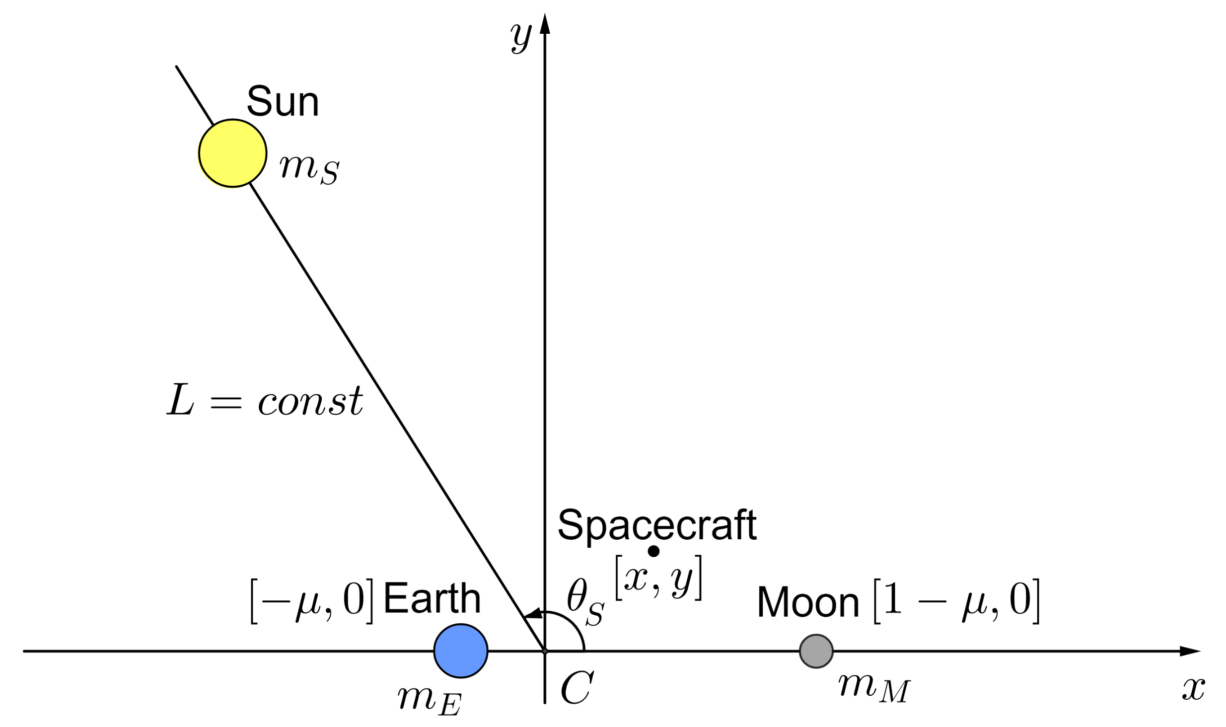
It is convenient to write ${\mathsf{\Omega }}_S$ and its derivative $\partial {\mathsf{\Omega }}_S/\partial {\theta }_S$ in the Sun–barycenter frame with the $x^{\prime }$-axis directed along the line connecting the Sun and the Earth–Moon barycenter (Figure 5). Note that we retain the prime notation for the axes of this frame: the only difference from the Sun–Earth rotating reference frame of Figure 4 is a slight displacement of the origin from the Earth’s center to the Earth–Moon barycenter. If we introduce the polar coordinates $x^{\prime }=\rho cos\alpha$, $y^{\prime }=\rho sin\alpha$ in the $C{x}^{\prime }{y}^{\prime }$ plane and make use of the relations $r^2-z^2=x^2+y^2=x^{\prime 2}+y^{\prime 2}={\rho }^2$, $x=-\rho cos({\theta }_S+\alpha )$, $y=-\rho sin({\theta }_S+\alpha )$, Equation (6) is simplified to

$$r_3=\sqrt{L^2+r^2+2L\rho cos\alpha }.$$

Substituting in Equation (5) and taking into account $\rho /L\le r/L\ll 1$ yields

$${\mathsf{\Omega }}_S=\frac{G{m}_S}{\sqrt{L^2+r^2+2L\rho cos\alpha }}+\frac{G{m}_S}{L^2}\rho cos\alpha \approx \frac{G{m}_S}{L}-\frac{G{m}_S}{2L^3}{r}^2+\frac{3G{m}_S}{2L^3}{\rho }^2{cos}^2\alpha .$$

Finally, the partial derivative of ${\mathsf{\Omega }}_S$ with respect to ${\theta }_S$ equals minus the partial derivative with respect to $\alpha$:

$$\frac{\partial {\mathsf{\Omega }}_S}{\partial {\theta }_S}=-\frac{\partial {\mathsf{\Omega }}_S}{\partial \alpha }\approx \frac{3}{2}\frac{G{m}_S}{L^3}{\rho }^{2}sin2\alpha .$$

(10)

To reduce the spacecraft’s orbital energy and ensure ballistic capture, the Sun’s gravitational perturbation should lead to the positive increment of the Earth–Moon Jacobi integral. The predominant contribution to such an increment is due to the integral term in Equation (9): the spacecraft spends many weeks near the apogee of a SALT trajectory where ${\rho }^2\simeq 10$. In order for the integral

$$\int \frac{\partial {\mathsf{\Omega }}_S}{\partial {\theta }_S}d{\theta }_S=\int \frac{\partial {\mathsf{\Omega }}_S}{\partial {\theta }_S}{\omega }_{S}dt$$

to be positive, the partial derivative (10) should be negative. This is equivalent to the inequality $sin2\alpha <0$ valid for either the second or the fourth quadrant of the Sun–barycenter reference frame.

So, using simple considerations, we have proven analytically the well-known quadrant rule observed by researchers when numerically designing SALT trajectories. Note that so far we did not assume a Sun-assisted transfer trajectory to be planar.

The quadrant rule will be useful for us later for the purpose of analyzing the features of designed SALT trajectories.

3.2. The $L_2$ Lunar Gateway

It is convenient to design a SALT trajectory in reverse order, starting with the arriving leg. At this phase of flight, exterior ballistic capture happens: the spacecraft “dives” into the $L_2$ neck of the zero-velocity surface. In the planar Earth–Moon CR3BP, the integral manifold $\mathcal{J}\left(\tilde{J}\right)$ for low-energy values of $\tilde{J}$ (that is, $3<J_{L3}\le \tilde{J}\le J_{L2}$; see also Appendix A.1 about the critical values of the Jacobi integral) is divided into two non-overlapping parts by the stable invariant manifold of the planar Lyapunov orbit with the same value of $\tilde{J}$ [3,36], and ballistic capture can occur in a planar SALT trajectory only if its arriving leg belongs to the interior of the corresponding two-dimensional stable manifold tube (Figure 6).

In the $(x,\dot{x})$ plane, manifold trajectories, when crossing the Earth–Moon RoP boundary, form a closed curve limiting the $L_2$ lunar gateway (Figure 7). Let G denote a set of inner points of the gateway. For any point $[x_P,{\dot{x}}_P]$ of the gateway, the corresponding coordinate $y_P$ may be found from the condition of belonging to the RoP boundary; after that, ${\dot{y}}_P$ is determined by the energy constraint $J(x_P,y_P,{\dot{x}}_P,{\dot{y}}_P)=\tilde{J}$. The closer $\tilde{J}$ to $J_{L2}$, the smaller the lunar gateway, shrinking to a single point at $J=J_{L2}\approx 3.184$ (see Figure 8). Thus, inserting the spacecraft into any circumlunar orbit with $J>3.184$ is impossible without additionally performing a lunar orbit insertion maneuver.

The numerical propagation of any initial condition $[x_P,y_P,{\dot{x}}_P,{\dot{y}}_P]$ in the CR3BP model generates a ballistic capture trajectory (Figure 6) passing by the Moon at a selenocentric distance $r_{\pi }$, with the argument of perilune ${\omega }_{\pi }$ (in the planar case, it stands for the angle between the $Cx$ axis of the Earth–Moon rotating reference frame and the Moon–perilune line). The points corresponding to a specified value of $r_{\pi }$ can be grouped in a single gradient-colored contour line. Figure 9 shows such a line for $r_{\pi }=3141$ km on the $L_2$ lunar gateway with $J=3.06$. The color along the line indicates the ${\omega }_{\pi }$ value for the associated ballistic capture trajectory. If we want the arriving leg to have specific values of $r_{\pi }$ and ${\omega }_{\pi }$, the corresponding gateway point should be targeted. If the Jacobi integral value of the desired (nominal) lunar orbit is greater than $J_{L2}$, the spacecraft has to enter a gateway with $J\lesssim J_{L2}$ and then perform an LOI burn.

To estimate a perilune impulse required to insert the spacecraft in a nominal lunar orbit with $J>J_{L2}$, one can use the approximate expression $J\approx 3(1-\mu )+2W_z-2E$ for the Jacobi integral via the osculating elements in the Moon-centered inertial frame (see Appendix A.2). Here, $W_z$ is the z-component of the orbital angular momentum and E is the Keplerian energy of the spacecraft’s capture orbit around the Moon. For the planar motion, this expression can be rewritten in terms of the perilune distance $r_{\pi }$ and the spacecraft velocity at perilune $V_{\pi }$ as $J=3(1-\mu )\pm 2r_{\pi }{V}_{\pi }-V_{\pi }^2+2\mu /r_{\pi }$ (the inertial spacecraft velocity relative to the Moon is assumed). The sign of the second term shows whether the orbit is direct or retrograde. Thus, the required LOI burn at perilune can be determined from the quadratic equation

$$\Delta J=\pm 2r_{\pi }\Delta V_{\pi }-2V_{\pi }\Delta V_{\pi }-{(\Delta V_{\pi })}^2,$$

(11)

where $\Delta J=J_{\mathrm{nom}}-J_{\mathrm{arr}}$ is the Jacobi integral increment (the difference between its values for a nominal orbit and for the arriving leg). Among the two negative roots, we are interested in the one with the least magnitude $\Delta V=|\Delta V_{\pi }|$. Such a magnitude is given by the formula

$$\Delta V=V_{\pi }\mp r_{\pi }-\sqrt{{(V_{\pi }\mp r_{\pi })}^2-\Delta J}.$$

(12)

This estimate of the LOI burn magnitude, though accurate enough, can be further improved when adapting the trajectory to more realistic dynamical models.

3.3. Exterior Leg Backward Propagation

Once a point of some $L_2$ lunar gateway is selected, the exterior leg can be reconstructed directly in the BR4BP by propagating the point backward in time until the trajectory re-enters the Earth–Moon RoP (or until the predefined maximum propagation time, set to 250 days in this work, is reached). The Sun’s phase at the beginning of the propagation is to be specified.

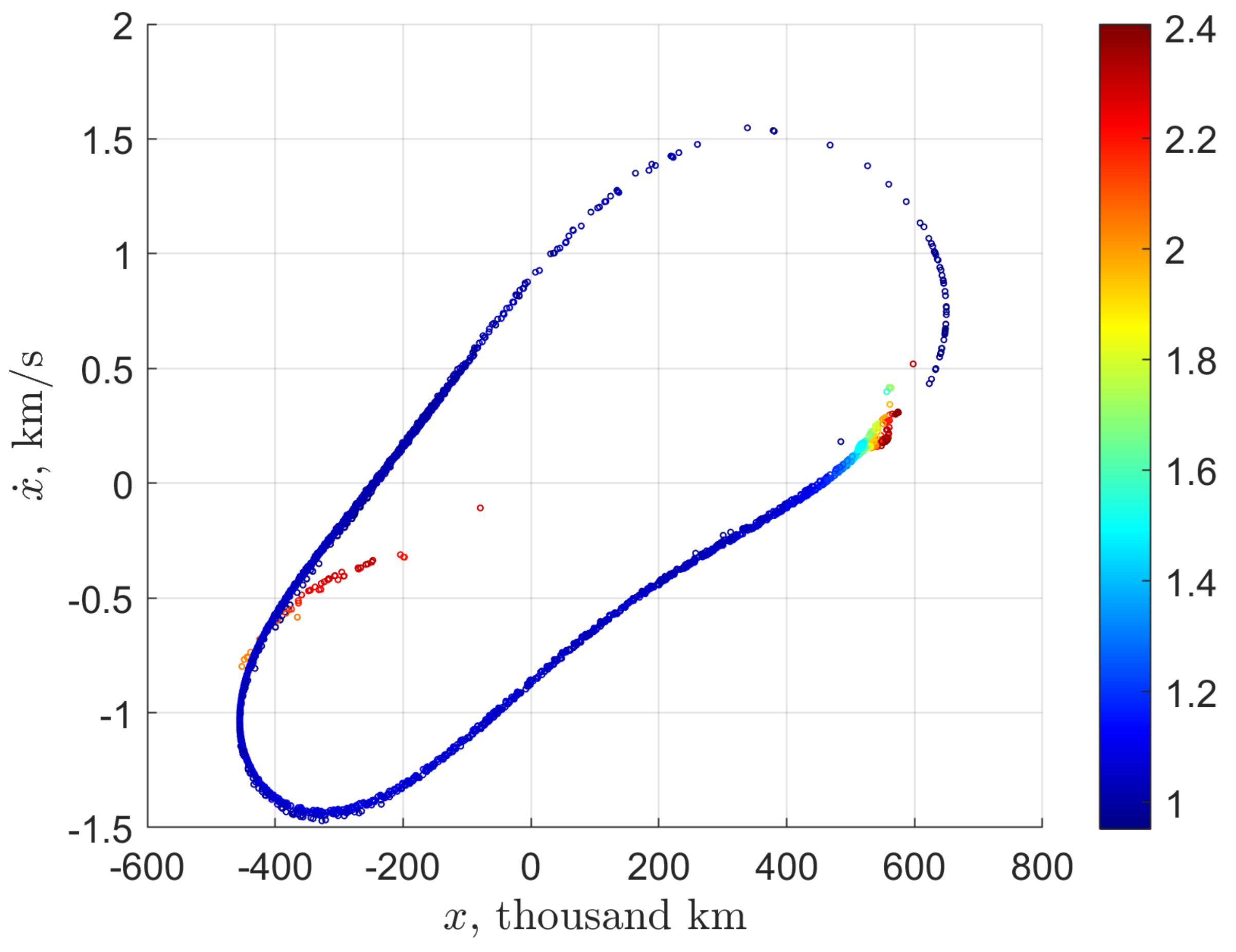
To demonstrate the abundance of SALT trajectories, we restrict ourselves to just a single contour line, the one shown in Figure 9. Propagating more than a thousand points along the contour line with 1500 different values of the Sun’s phase in the $[0,2\pi ]$ interval, we obtained almost 287 thousand potential exterior legs (about 14% of the propagated trajectories). Their phase states at crossing the Earth–Moon RoP boundary can be visualized on the $(x,\dot{x})$ plane (Figure 10). As earlier, the y-coordinate is readily retrieved from Equation (8), then $\dot{y}$ can be recovered from the Jacobi integral value at the RoP re-entry, which is indicated by the color. The lower this value, the more pronounced was the solar gravity perturbation effect along the exterior leg. Meanwhile, we do not display the points with $J>2.47$ because such exterior legs cannot be in principle patched with any departing leg: the corresponding launch energy $C_3$, according to Equation (A19) from Appendix A.2, appears to be less than −2.17 km²/s², which is not enough for the spacecraft to reach the Moon and/or exit the Earth–Moon region of prevalence (after the TLI burn, the apogee distance would be less than 367,000 km).

3.4. Translunar Injection Maneuver Design

To calculate the departing leg, one has to select the translunar injection burn magnitude and the point at a given low-Earth parking orbit where the TLI impulse is applied. The range the impulse magnitude should belong to is defined by the Jacobi integral range of candidate exterior legs. For example, in the 200 km parking orbit, the TLI burn ensuring $J\in [0.95,2.41]$ has a magnitude between 3.13 km/s and 3.20 km/s. The location of performing the TLI burn in the parking orbit can be parameterized by, say, the phase angle $\theta$, counting from the x-axis of the Earth–Moon rotating frame. Alternatively, the angle $\alpha$, counted from the $x^{\prime }$-axis of the Sun–barycenter frame, may be used. These angles are related to each other by the expression $\theta =\alpha +{\theta }_S-\pi mod2\pi$ (see Figure 5). Note that both angles can be more conveniently defined with respect to the geocentric (rather than barycentric) rotating frame and the above relationship still keeps valid—the angles simply decrease by the same amount, whereas the solar phase ${\theta }_S$ almost does not change (see Appendix B). Below, this convention is assumed.

We have propagated more than a hundred thousand potential departing legs by taking different values of the TLI burn magnitude and phase (from the estimated interval and from $[0,2\pi ]$, respectively). A departing leg was considered patched with some candidate exterior leg if, leaving the Earth–Moon RoP, it has almost the same phase state (the norm difference of ${10}^{-2}$ was tolerated). As a result, we succeeded in patching more than 3000 pairs of exterior and departing legs. The corresponding “survived” points of Figure 10 are displayed in Figure 11.

3.5. Classification and Features of Patched SALT Trajectories

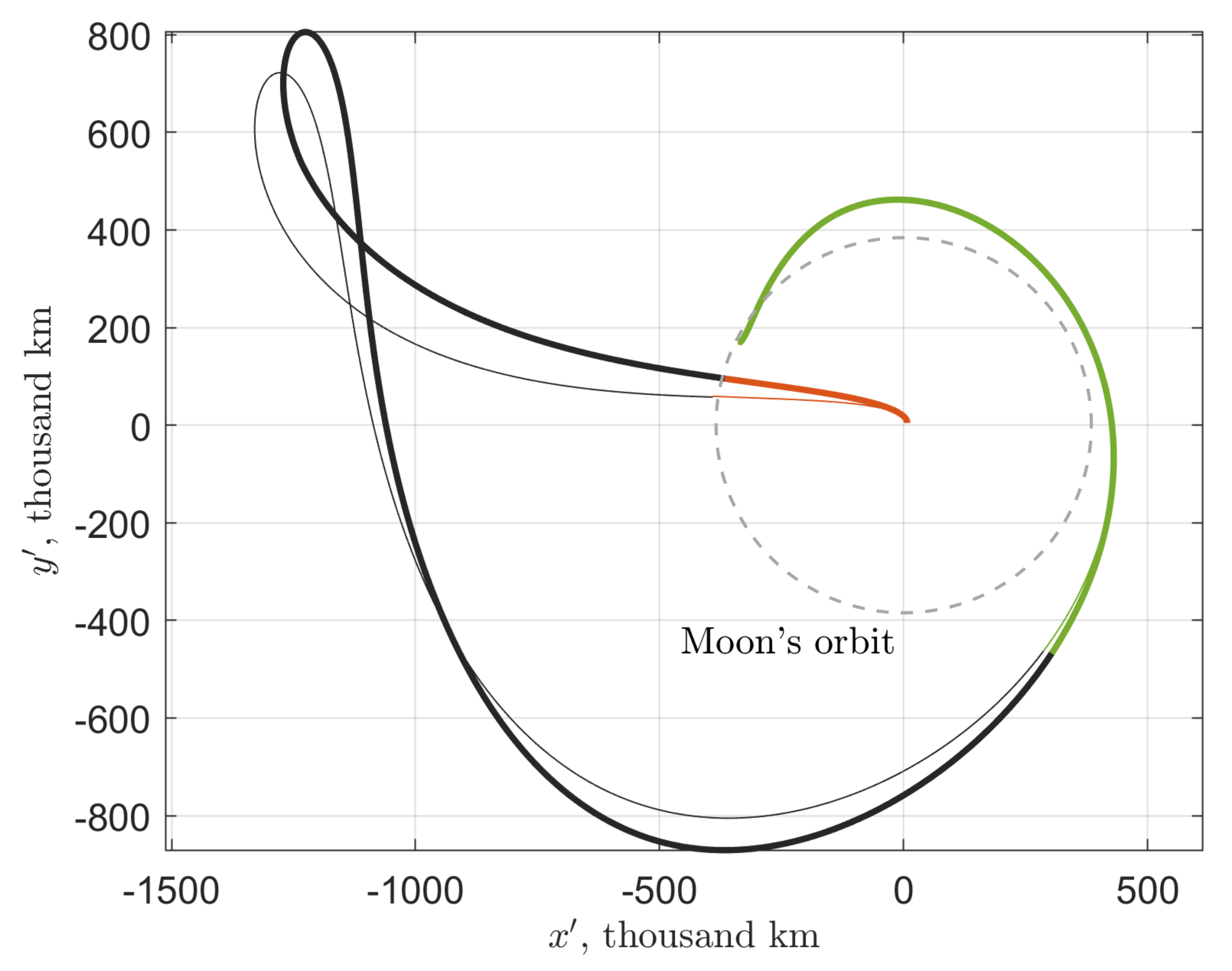
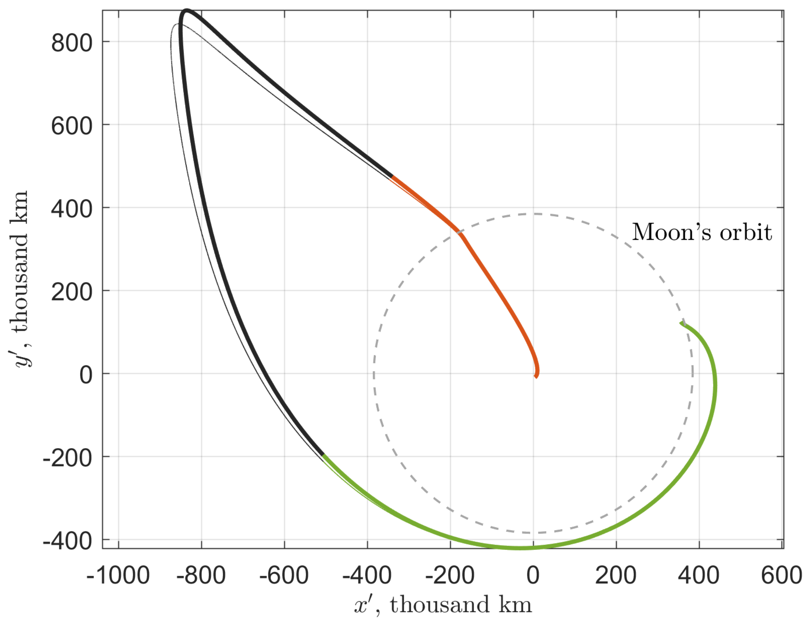
Let us classify and characterize the patched SALT trajectories we obtained. They all can be grouped into three categories, depending on the existence and type of an intermediate lunar flyby on the departing leg. Sample trajectories of each type are shown in Figure 12. The first type is comprised of SALT trajectories not approaching the Moon closer than 60,000 km on the departing leg (no flyby). The other two types of trajectories (which amount to 14% of the whole database of patched SALT trajectories) include a lunar flyby.

For a second-type SALT trajectory (see Figure 13), the spacecraft crosses the x-axis in front of the Moon (when observing from the Earth) and has a positive orbital angular momentum $w_z$ in the rotating frame at the moment of flyby. We will thus further refer to such a flyby as direct (note that in [31,33] it is called a trailing side flyby). On the contrary, a SALT trajectory of the third type (Figure 14) includes a retrograde flyby (a leading side flyby in [31,33])—the spacecraft crosses the x-axis behind the Moon and has a negative orbital angular momentum. As can be readily deduced from Equation (A12) of Appendix A.2, the orbital angular momentum in the rotating frame $w_z$ is related to its inertial-frame counterpart $W_z$ at an arbitrary moment by the simple expression $W_z=w_z+r_2^2$. Particularly, at the moment of flyby, we have $W_z=w_z+r_{\pi }^2$. If the flyby distance $r_{\pi }\ll 1$, then $W_z\approx w_z$.

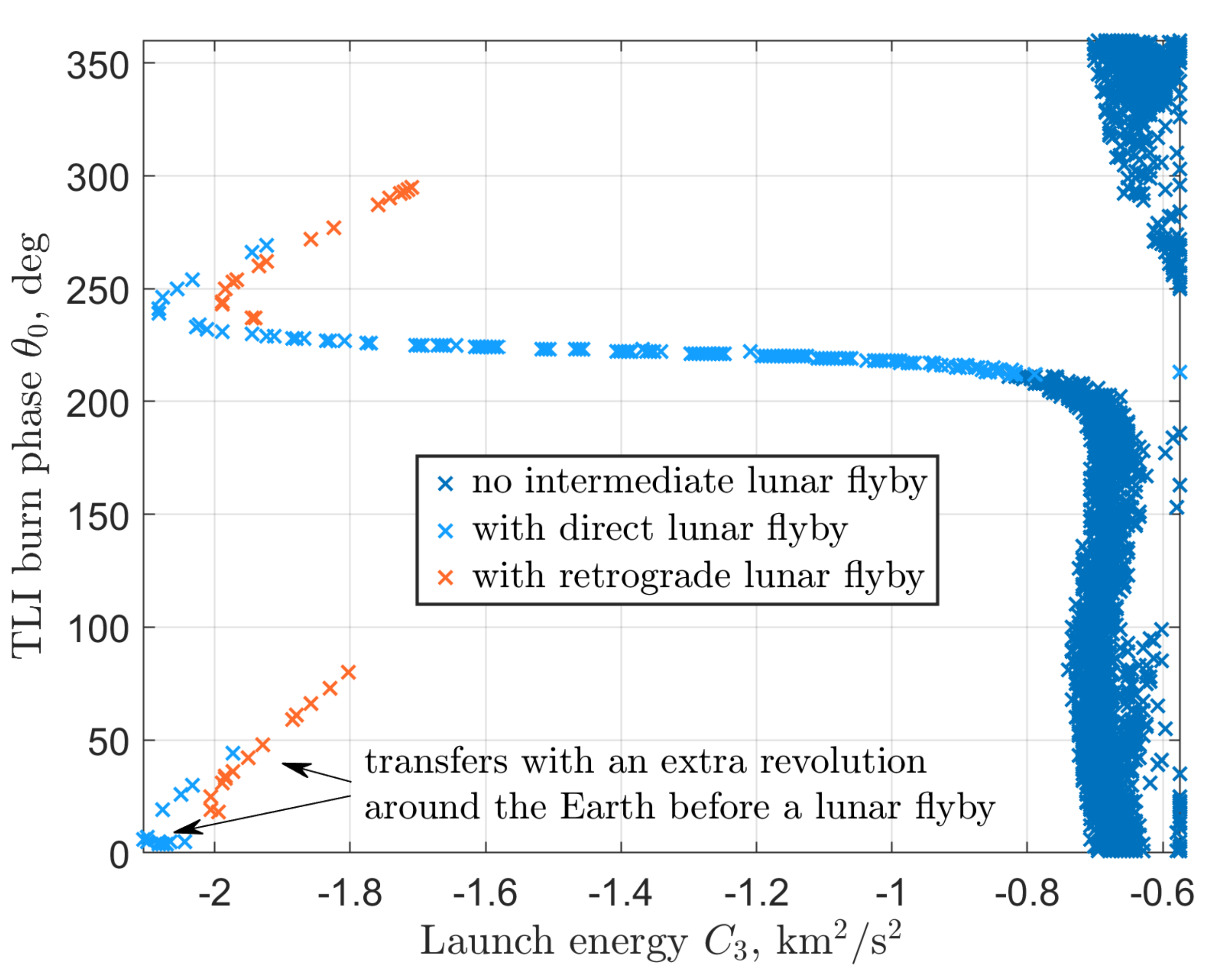
It is convenient that the initial conditions (the launch energy $C_3$ and the TLI burn phase) for the patched SALT trajectories almost do not depend on a specific low-Earth parking orbit and can be visualized in a single chart (Figure 15). Excluding transfers with an extra revolution around the Earth before an intermediate lunar flyby, one can conclude that SALT trajectories of the second or third type require executing the TLI maneuver at a point in the parking orbit in which phase ${\theta }_0$ is in the range of $215\dots 295$ deg. The lower part of this range ($215\dots 225$ deg) corresponds to second-type trajectories, while the TLI burn phase of third-type trajectories is bounded between 235 deg and 295 deg. As expected, no-flyby trajectories do not exhibit any pattern in ${\theta }_0$ and require a launch energy of at least −0.8 km²/s² (the TLI impulse of about 3.19 km/s in the 200 km parking orbit). Including an intermediate flyby allows one to reduce the launch energy as low as up to −2.1 km²/s².

For all three types of SALT trajectories, the initial Sun–Earth–spacecraft geometry is predictably crucial. It is expressed the most in terms of the TLI burn polar angle ${\alpha }_0$ relative to the Sun–Earth line. The majority of trajectories with a direct lunar flyby demand this angle to be approximately either 130 deg or 310 deg (see Figure 16). The former case corresponds to fourth quadrant trajectories, whereas the latter is for second quadrant trajectories. The burn angle for trajectories with a retrograde flyby is about 60 deg (for second quadrant trajectories) or close to 240 deg (for fourth quadrant trajectories). The pattern is even more pronounced for no flyby trajectories: one can observe almost identical parts of the distribution, shifted by 180 deg with respect to each other and having peaks at 160 deg and 340 deg (Figure 17).

Since the TLI burn phase ${\theta }_0$ for second-type and third-type trajectories should belong to a certain range (it is especially narrow for trajectories with a direct flyby), no wonder that the Sun’s initial phase ${\theta }_{S,0}={\theta }_0-{\alpha }_0+\pi mod2\pi$ also tends to be grouped around some values. For example, two distinct peaks of second-type trajectories are located at 95 deg and 275 deg (Figure 18). When speaking of the transfer duration, most of the first-type trajectories complete a low-energy transfer in less than 3 months (see Figure 19). Trajectories with a direct flyby exhibit almost the same performance, with those with a smaller $C_3$ being slower. Finally, trajectories with a retrograde flyby generally require more time, from 4 to 6 months (Figure 20).

3.6. Adaptation to More Complex Dynamical Models

Patched SALT trajectories are easily adaptable to the BR4BP model. When a single midcourse correction is allowed to be performed at the apogee of a SALT trajectory, the standard multiple-shooting procedure appears to work very well: a trajectory can be rapidly adapted by adjusting only the TLI impulse magnitude and phase and possibly adding a small apogee trajectory correction maneuver (TCM). The departure and arrival times (or, equivalently, the solar phase values at the departure/arrival epochs) are allowed to be fixed.

Three examples of SALT trajectories before and after adaptation for each type of Sun-assisted transfers are depicted in Figure 21, Figure 22 and Figure 23. In all the examples, the TLI burn magnitude changes by at most several m/s and its phase shift is in the order of a couple of degrees. The apogee correction maneuvers vary from 0.6 m/s for the second-type (direct flyby) trajectory to 34.5 m/s for the third-type (retrograde flyby) trajectory.

Converting a planar SALT trajectory to a three-dimensional transfer trajectory in a high-fidelity ephemeris model is a separate problem beyond the scope of this paper. However, the remark can be made that such a numerical procedure is almost always based on some sort of multiple-shooting method. While for trajectories in the three-dimensional BR4BP model the shooting is essentially straightforward [33], the adaptation of planar trajectories is involved. It often demands additional steps: to first generate an intermediate quasi-planar trajectory in the ephemeris model [37] or to gradually deform a trajectory (the homotopic approach).

4. Conclusions and Future Work

The proposed methodology of dividing a planar SALT trajectory into several parts with different dynamics is analogous to the patched conic approximation concept for high-energy trajectories. It appears fruitful in classifying SALT trajectories, identifying basic features (TLI burn magnitudes and phases, initial solar phase values, etc.), and quantifying the perturbing effect due to the Sun’s gravity to rigorously prove the quadrant rule. The $L_2$ lunar gateway is a convenient tool for targeting specific capture conditions. In the next step of the study, we will examine several gateways with other Jacobi integral values in order to fully understand the behavior of SALT trajectories of all three types. It opens the road to the semianalytical design of planar SALT trajectories: by properly setting the departure parameters, one will be able to generate an excellent initial guess from which the multiple-shooting procedure could rapidly converge to a planar BR4BP trajectory with the desired characteristics.

The numerically observed similarity of planar and spatial SALT trajectories (in terms of their geometric shapes and principal parameters) gives us a reasonable hope that most of the results obtained in the planar case could be transferred (or naturally extended) to the spatial BR4BP model. Ideally, a unified multiple-shooting method and the general rules of choosing the initial conditions should be developed for both planar and spatial SALT trajectories. The transition from the BR4BP to the ephemeris model would then be a simple final step.

References

1. Gill, T. Lunar Orbital Platform-Gateway. In Proceedings of the 45th Space Congress, Cape Canaveral, FL, USA, 27 February–1 March 2018. [Google Scholar]
2. Egorov, V.A. Certain Problems of Moon Flight Dynamics. Russ. Lit. Satell. 1958, 1, 107–174. [Google Scholar]
3. Conley, C.C. Low Energy Transit Orbits in the Restricted Three-Body Problem. SIAM J. Appl. Math. 1968, 16, 732–746. [Google Scholar] [CrossRef]
4. Racca, G.D.; Marini, A.; Stagnaro, L.; Van Dooren, J.; Di Napoli, L.; Foing, B.H.; Lumb, R.; Volp, J.; Brinkmann, J.; Grünagel, R.; et al. SMART-1 Mission Description and Development Status. Planet. Space Sci. 2002, 50, 1323–1337. [Google Scholar] [CrossRef]
5. Belbruno, E.; Miller, J. A Ballistic Lunar Capture Trajectory for the Japanese Spacecraft Hiten; Technical Report IOM 312/90.4-1731-EAB; Jet Propulsion Laboratory (JPL), California Institute of Technology: Pasadena, CA, USA, 1990. [Google Scholar]
6. Belbruno, E.A.; Miller, J.K. Sun-Perturbed Earth-to-Moon Transfers with Ballistic Capture. J. Guid. Control Dyn. 1993, 16, 770–775. [Google Scholar] [CrossRef]
7. Ivashkin, V.V. On Trajectories of Earth–Moon Flight of a Particle with Its Temporary Capture by the Moon. Dokl. Phys. 2002, 47, 825–827. [Google Scholar] [CrossRef]
8. Topputo, F.; Belbruno, E.; Gidea, M. Resonant Motion, Ballistic Escape, and Their Applications in Astrodynamics. Adv. Space Res. 2008, 42, 1318–1329. [Google Scholar] [CrossRef]
9. Belbruno, E.; Topputo, F.; Gidea, M. Resonance Transitions Associated to Weak Capture in the Restricted Three-Body Problem. Adv. Space Res. 2008, 42, 1330–1351. [Google Scholar] [CrossRef]
10. Howell, K.; Barden, B.; Wilson, R.; Lo, M. Trajectory Design Using a Dynamical Systems Approach with Application to Genesis. In Proceedings of the AAS/AIAA Astrodynamics Specialist Conference, Sun Valley, ID, USA, 4–7 August 1997. [Google Scholar]
11. Koon, W.; Lo, M.; Marsden, J.; Ross, S. Low Energy Transfer to the Moon. Celest. Mech. Dyn. Astron. 2001, 81, 63–73. [Google Scholar] [CrossRef]
12. Gómez, G.; Koon, W.; Lo, M.; Marsden, J.; Masdemont, J.; Ross, S. Invariant Manifolds, the Spatial Three-Body Problem and Space Mission Design. In Proceedings of the AIAA/AAS Astrodynamics Specialist Meeting, Quebec City, QC, Canada, 30 July–2 August 2001. [Google Scholar]
13. Parker, J.; Born, G. Modeling a Low-Energy Ballistic Lunar Transfer Using Dynamical Systems Theory. J. Spacecr. Rocket. 2008, 45, 1269–1281. [Google Scholar] [CrossRef]
14. Ross, S.D.; Scheeres, D.J. Multiple Gravity Assists, Capture, and Escape in the Restricted Three-Body Problem. SIAM J. Appl. Dyn. Syst. 2007, 6, 576–596. [Google Scholar] [CrossRef] [Green Version]
15. Grover, P.; Ross, S. Designing Trajectories in the Planet-Moon Environment Using the Controlled Keplerian Map. J. Guid. Control Dyn. 2009, 32, 436–443. [Google Scholar] [CrossRef] [Green Version]
16. Campagnola, S.; Russell, R.P. Endgame Problem Part 2: Multibody Technique and the Tisserand-Poincaré Graph. J. Guid. Control Dyn. 2010, 33, 476–486. [Google Scholar] [CrossRef]
17. Lantoine, G.; Russell, R.P.; Campagnola, S. Optimization of Low-Energy Resonant Hopping Transfers between Planetary Moons. Acta Astronaut. 2010, 68, 1361–1378. [Google Scholar] [CrossRef]
18. García, F.; Gómez, G. A Note on Weak Stability Boundaries. Celest. Mech. Dyn. Astron. 2007, 97, 87–100. [Google Scholar] [CrossRef]
19. Belbruno, E.; Gidea, M.; Topputo, F. Weak Stability Boundary and Invariant Manifolds. SIAM J. Appl. Dyn. Syst. 2010, 9, 1061–1089. [Google Scholar] [CrossRef] [Green Version]
20. Roncoli, R.; Fujii, K. Mission Design Overview for the Gravity Recovery and Interior Laboratory (GRAIL) Mission. In Proceedings of the AIAA/AAS Astrodynamics Specialist Conference, Toronto, ON, Canada, 2–5 August 2010. [Google Scholar]
21. Parker, J.S.; Cheetham, B.; Gardner, T.; Thompson, M.; Forsman, A.; Kayser, E.; Ott, C.; Kam, A.; Baskar, S.; Bolliger, M.; et al. CAPSTONE: Pathfinder for the Lunar Gateway. In Proceedings of the 73rd International Astronautical Congress, Paris, France, 18–22 September 2022. [Google Scholar]
22. Korean Aerospace Research Institute. Korea’s First Step toward Lunar Exploration. Available online: https://www.kari.re.kr/eng/sub03_07_01.do (accessed on 12 March 2023).
23. Folta, D.; Bosanac, N.; Cox, A.; Howell, K. The Lunar IceCube Mission Design: Construction of Feasible Transfer Trajectories with a Constrained Departure. Adv. Astronaut. Sci. 2016, 158, 1352–1369. [Google Scholar]
24. Oguri, K.; Oshima, K.; Campagnola, S.; Kakihara, K.; Ozaki, N.; Baresi, N.; Kawakatsu, Y.; Funase, R. EQUULEUS Trajectory Design. J. Astronaut. Sci. 2020, 67, 950–976. [Google Scholar] [CrossRef]
25. Topputo, F. On Optimal Two-Impulse Earth–Moon Transfers in a Four-Body Model. Celest. Mech. Dyn. Astron. 2013, 117, 279–313. [Google Scholar] [CrossRef] [Green Version]
26. Oshima, K.; Topputo, F.; Campagnola, S.; Yanao, T. Analysis of Medium-Energy Transfers to the Moon. Celest. Mech. Dyn. Astron. 2017, 127, 285–300. [Google Scholar] [CrossRef]
27. Oshima, K.; Topputo, F.; Yanao, T. Low-Energy Transfers to the Moon with Long Transfer Time. Celest. Mech. Dyn. Astron. 2019, 131, 1–19. [Google Scholar] [CrossRef]
28. Parrish, N.L.; Kayser, E.; Bolliger, M.J.; Thompson, M.R.; Parker, J.S.; Cheetham, B.W.; Davis, D.C.; Sweeney, D.J. Ballistic Lunar Transfers to Near Rectilinear Halo Orbit: Operational Considerations. In Proceedings of the AIAA SciTech Forum, Orlando, FL, USA, 6–10 January 2020. [Google Scholar]
29. Scheuerle, S.T.; Howell, K.C. Characteristics and Analysis of Families of Low-Energy Ballistic Lunar Transfers. In Proceedings of the AAS/AIAA Astrodynamics Specialist Conference, Big Sky, MT, USA, 9–11 August 2021. [Google Scholar]
30. Rosales, J.J.; Jorba, À.; Jorba-Cuscó, M. Transfers from the Earth to L2 Halo Orbits in the Earth–Moon Bicircular Problem. Celest. Mech. Dyn. Astron. 2021, 133, 1–20. [Google Scholar]
31. McCarthy, B.P.; Howell, K.C. Ballistic Lunar Transfer Design to Access Cislunar Periodic and Quasi-Periodic Orbits Leveraging Flybys of the Moon. In Proceedings of the 72nd International Astronautical Congress, Dubai, United Arab Emirates, 25–29 October 2021. [Google Scholar]
32. McCarthy, B.; Howell, K.C. Characterization of Families of Low-Energy Transfers to Cislunar Four-Body Quasi-Periodic Orbits. In Proceedings of the AIAA SciTech Forum, San Diego, CA, USA, 4–6 January 2022. [Google Scholar]
33. McCarthy, B.; Howell, K.C. Four-Body Cislunar Quasi-Periodic Orbits and Their Application to Ballistic Lunar Transfer Design. Adv. Space Res. 2023, 71, 556–584. [Google Scholar] [CrossRef]
34. Scheuerle, S.; Howell, K.C.; Davis, D. Low Thrust Augmentation for Ballistic Lunar Transfers. In Proceedings of the 33rd AAS/AIAA Space Flight Mechanics Meeting, Austin, TX, USA, 8–12 January 2023. [Google Scholar]
35. Castelli, R. Regions of Prevalence in the Coupled Restricted Three-Body Problems Approximation. Commun. Nonlinear Sci. Numer. Simul. 2012, 17, 804–816. [Google Scholar] [CrossRef]
36. Parker, J.; Anderson, R. Low-Energy Lunar Trajectory Design; John Wiley & Sons: Hoboken, NJ, USA, 2013; p. 13. [Google Scholar]
37. Tselousova, A.; Trofimov, S.; Shirobokov, M. Multiple-Shooting Continuation of Sun-Assisted Lunar Transfers from the Planar Bicircular to the Ephemeris Model. In Proceedings of the 73rd International Astronautical Congress, Paris, France, 18–22 September 2022. [Google Scholar]
Figure 1. Rotating reference frame in the Earth–Moon circular restricted three-body problem.
Applsci 13 04676 g001
Figure 2. Rotating reference frame in the Earth–Moon–Sun bicircular restricted four-body problem. The figure is drawn for the planar case (the z-coordinate is dropped), though also valid in the 3D case.
Applsci 13 04676 g002
Figure 3. Earth–Moon region of prevalence boundaries for different Sun phase angles and the elliptical boundary of the mean-square averaged region of prevalence (bold orange).
Applsci 13 04676 g003
Figure 4. Examples of planar SALT trajectories in the BR4BP with the departing (red), arriving (green) and exterior (black) legs patched on the boundary of the Earth–Moon region of prevalence. The orbit of the Moon is marked by the dashed gray line. The apogee of every SALT trajectory in the Earth-centered Sun–Earth rotating frame is located in the 2nd or 4th quadrant.
Applsci 13 04676 g004
Figure 5. Earth–Moon and Sun–barycenter rotating reference frames C x y and C x y . The radius vector of the spacecraft in the Sun–barycenter frame is described by the polar angle α .
Applsci 13 04676 g005
Figure 6. Sample ballistic capture trajectory with the closest lunar approach of 1403 km ( r π = 3141 km) at a point with ω π = 83.5 deg. The Jacobi integral value equals J = 3.06 along the capture trajectory.
Applsci 13 04676 g006
Figure 7. L 2 lunar gateway G in the ( x , x ˙ ) plane. The region is formed by stable manifold trajectories of the J = 3.06 planar Lyapunov orbit when crossing the Earth–Moon RoP boundary.
Applsci 13 04676 g007
Figure 8. Nested L 2 lunar gateways for different Jacobi integral levels: J = 3.06 , J = 3.10 , J = 3.15 .
Applsci 13 04676 g008
Figure 9. L 2 lunar gateway for J = 3.06 with the r π = 3141 km perilune distance contour line marked. Targeting point P results in the trajectory shown in Figure 6 (the argument of perilune ω π = 83.5 deg).
Applsci 13 04676 g009
Figure 10. Earth–Moon RoP re-entry conditions for candidate exterior legs. The color reflects the Jacobi integral value at re-entry. The points with J > 2.47 are not displayed because it is unfeasible to patch the associated exterior legs with any departing leg.
Applsci 13 04676 g010
Figure 11. Earth–Moon RoP re-entry conditions corresponding to the exterior legs successfully patched with a departing leg. The color reflects the Jacobi integral value at re-entry.
Applsci 13 04676 g011
Figure 12. Three types of SALT trajectories: (I) without any intermediate lunar flyby, (II) with a direct lunar flyby, (III) with a retrograde lunar flyby. The Moon’s orbit is marked by the dashed gray line.
Applsci 13 04676 g012
Figure 13. Sample departing leg with a direct lunar flyby. The orbital angular momentum with respect to the Moon in the rotating frame is positive; the spacecraft crosses the x-axis in front of the Moon.
Applsci 13 04676 g013
Figure 14. Sample departing leg with a retrograde lunar flyby. The orbital angular momentum relative to the Moon in the rotating frame is negative; the spacecraft crosses the x-axis behind the Moon.
Applsci 13 04676 g014
Figure 15. Initial conditions (the launch energy C 3 and the TLI burn phase) corresponding to the three types of SALT trajectories: without an intermediate flyby (blue), with a direct lunar flyby (light blue), or with a retrograde lunar flyby (red).
Applsci 13 04676 g015
Figure 16. Distribution of spacecraft polar angle values at the moment of TLI burn execution for SALT trajectories including a lunar flyby. Two distinct peaks at about 130 deg and 310 deg correspond to the 4th and 2nd quadrant trajectories with a direct flyby. The burn angle for retrograde flyby trajectories can be either close to 60 deg (2nd quadrant trajectories) or about 240 deg (4th quadrant trajectories).
Applsci 13 04676 g016
Figure 17. Distribution of spacecraft polar angle values at the moment of TLI burn execution for SALT trajectories without an intermediate lunar flyby. Two peaks at about 160 deg and 340 deg correspond to the 4th and 2nd quadrant trajectories. The pattern is repeated almost exactly when shifting by 180 deg.
Applsci 13 04676 g017
Figure 18. Distribution of solar phase angles at the moment of TLI burn execution for SALT trajectories with a lunar flyby. Two distinct peaks at about 95 deg and 275 deg correspond to the 2nd and 4th quadrant trajectories with a direct flyby. For retrograde flyby trajectories, the pattern is not so clear, but small peaks around 140 deg and 350 deg values could be identified.
Applsci 13 04676 g018
Figure 19. Distribution of the total transfer duration for SALT trajectories without a lunar flyby.
Applsci 13 04676 g019
Figure 20. Distribution of the total transfer duration for SALT trajectories including a lunar flyby.
Applsci 13 04676 g020
Figure 21. A sample SALT trajectory of the first type (no flyby): the patched three-body approximation (thin) and upon adaptation to the BR4BP (bold). The segments of the adapted trajectory corresponding to the departing, arriving, and exterior legs, are colored the same (red, green, and black, respectively). In the course of adaptation, the TLI impulse has increased from 3193 m/s to 3194 m/s. The burn phase has changed from 97.35 deg to 103.01 deg. The apogee TCM of 12.7 m/s has been added.
Applsci 13 04676 g021
Figure 22. A sample SALT trajectory of the second type (with a direct lunar flyby): the patched three-body approximation (thin) and upon adaptation to the BR4BP (bold). As earlier, the adapted trajectory segments corresponding to the departing, arriving, and exterior legs, are colored the same (red, green, and black, respectively). Upon adaptation, the TLI burn has increased from 3163 m/s to 3166 m/s. The burn phase has changed from 221.84 deg to 221.43 deg. The apogee TCM of 0.6 m/s has been added.
Applsci 13 04676 g022
Figure 23. A sample SALT trajectory of the third type (with a retrograde lunar flyby): the patched three-body approximation (thin) and upon adaptation to the BR4BP (bold). As earlier, the adapted trajectory segments corresponding to the departing, arriving, and exterior legs, are colored the same (red, green, and black, respectively). Upon adaptation, the TLI burn has decreased from 3149 m/s to 3147 m/s. The burn phase has changed from 296.84 deg to 293.88 deg. The apogee TCM of 34.5 m/s has been added.
Applsci 13 04676 g023
Disclaimer/Publisher’s Note: The statements, opinions and data contained in all publications are solely those of the individual author(s) and contributor(s) and not of MDPI and/or the editor(s). MDPI and/or the editor(s) disclaim responsibility for any injury to people or property resulting from any ideas, methods, instructions or products referred to in the content.