Abstract
Language models based on deep learning showed promising results for artistic generation purposes, including musical generation. However, the evaluation of symbolic musical generation models is mostly based on low-level mathematical metrics (e.g., the result of the loss function) due to the inherent difficulty in measuring the musical quality of a given performance due to the subjective nature of music. This work sought to measure and evaluate musical excerpts generated by deep learning models from a human perspective, limited to the scope of classical piano music generation. In this assessment, a population of 117 people performed blind tests with musical excerpts of human composition and musical excerpts generated using artificial intelligence models, including the models PerformanceRNN, Music Transformer, MuseNet and a custom model based on GRUs. The experiments demonstrated that musical excerpts generated using models based on the Transformer neural network architecture obtained the greatest receptivity within the tested population, surpassing the results of human compositions. In addition, the experiments also demonstrated that people with greater musical sensitivity and musical experience were more able to identify the compositional origin of the excerpts heard.
1. Introduction
Music is one of the universal aspects of all human societies. From tribes in the Amazon to small villages in the Chinese countryside, from ancient Greek society to contemporary digital society, humans use music as a means of expression. It is interesting to note that we can identify concepts in the musical structure that are similar to concepts in the linguistic structure, such as “phrases”, “stresses”, “punctuations”, and “sentences”.
Furthermore, as presented by Adorno and Gillespie [1], music also resembles a language in that both are a temporal succession of articulated sounds that are more than just a single sound and follow a certain coherence. Moreover, in both, we are highly sensitive to the subtleties and irregularities of these sequential data flows [2]. The comparison between music and language occurs naturally, considering that both involve complex sequences with meaning. From a neuroscience perspective, there is a growing body of evidence linking the way we perceive music and the way we perceive natural language [3]. On the other hand, natural language has been a much-discussed topic within the data world, considering the growing number of articles related to natural language processing (NLP) and models of deep artificial neural networks (deep learning). Among these studies, it is worth highlighting the problem of data-driven natural language generation, which is a topic that is currently the object of rigorous investigation by NLP researchers [4,5].
In addition, it is also worth noting the structural similarities between musical generation models and natural language generation models based on deep artificial neural networks. The model MuseNet presented by Payne (2019), which is developed by OpenAI, can be taken as an example. This model is based on the GPT-2 language model, also developed by OpenAI, and presented by Radford et al. (2019). Considering the structural similarities of the sequential nature of language and music, would it be possible for generative neural network architectures that are based on natural language models to express notions of harmony and melody pleasant enough to human ears? Would this musical content that is artificially generated by neural networks be robust enough to confuse a listener about its compositional origin? These questions served as a basis for the evolution of this work, which sought to explore and validate the result of the application of language models and generative neural network architectures for the purpose of algorithmic music composition.
The main goal of this study was to measure the musicality of musical excerpts generated using deep learning models from a human perspective. To achieve this objective, a population of 117 people, including musicians and non-musicians, was subjected to a blind test to evaluate the musicality of five different musical excerpts, with one human composition and four algorithmic compositions generated by deep learning models. The results of this research contribute with new information about how the musicality of the models differed from each other and how this musicality is perceived in relation to music of human compositional origin.
Another contribution of this article was showing that within the tested population, people with greater sensitivity or musical experience were more assertive in defining the compositional origin of the musical excerpts used. The source code of this study is publicly available in order to facilitate experimentation, access to the models and access to the data used in this research.
The paper continues with the exploration of materials and methods, where the details of data transformation and development of the models used are examined. This is followed by the definition of the structure of the blind test. After defining the resources and methodology, a discussion of the analysis and results of the blind test is given. Finally, the paper ends with the conclusions of the work.
2. Materials and Methods
Algorithmic music composition presents a challenging technical development. As described by Walder [2], unlike words that make up the data of a text, multiple musical notes can occur contemporaneously. To address this problem, generative models based on deep neural networks were used for music generation purposes through three types of different approaches:
- End-to-end model development (from data to inference).
- Partial model development using transfer learning through pre-trained model weights.
- Human–machine interaction through a web interface.
It is worth mentioning that the end-to-end model development approach relies on training techniques that were incorporated with the objective of maximizing the learning of the musical characteristics of the selected musical corpus. After training, the samples were generated in an auto-regressive way from the distributions estimated by the model, following the same modus operandi of the other models used. These distributions were compiled and transformed into musical excerpts, which served as the basis for the blind test, which sought to assess the musical quality of the model from a human perspective. From here, we can highlight the three main pillars for the development of this research, namely, the data, the models, and the blind test.
2.1. Data
There are multiple perspectives of data collection in relation to a musical artifact, starting from a more elementary approach, such as musical analysis of elements in a score, to more complex analyses starting from the raw sound wave of a certain audio file. This work focused on symbolic musical data based on the MIDI standard [6] within the musical scope of classical music.
The selection criterion for the dataset choice was based on the academic relevance in the domain of applied machine learning for music information retrieval (MIR). Among the listed sources, 3 main datasets were considered as potential candidates for the scope of this work, as follows:
Maestro: Introduced by Hawthorne et al. [7], Maestro is a music dataset containing over 200 h of virtuosic piano performance in MIDI format.
JSB Chorales: Introduced by Boulanger-Lewandowski et al. [8], the JSB choirs are a set of short musical pieces in four voices and are noted for their stylistic homogeneity. The chorales were originally composed by Johann Sebastian Bach in the 18th century. He wrote them by taking pre-existing melodies from contemporary Lutheran hymns and then harmonizing them to create the remaining three-voice parts. The version of the dataset used canonically in representational learning contexts consists of 382 of these chorals, with a training/validation/test split of 229, 76 and 77 samples, respectively.
MuseData: Also introduced by Boulanger-Lewandowski et al. [8], MuseData is an electronic library of classical orchestral and piano music from the Center for Computer-Assisted Research in the Humanities at Stanford University (CCARH). It consists of about 3 MB of 783 files.
However, even though these databases are within the same scope (classical music MIDI files), they have different structural natures. Maestro is a piano performance database, JSB Chorales is a 4-part choral database, and MuseData is a miscellaneous compilation of classical orchestral and piano music.
In order to achieve certain consistency within the distribution of information and the modeling process, the choice of a dataset with the minimum variation in its structural nature was chosen. The Maestro database was found to be the most appropriate within these criteria due to its consistency in terms of the structural organization of information since all elements of this database were derived from the same instrument (piano).
2.1.1. Data Augmentation
Data augmentation techniques for generating synthetic data were used to maximize the assertiveness of the models. These techniques were based on musical transposition and temporal transposition techniques. Musical transposition (or tonal transposition) changes the sequence of music notes to a harmonic field above or below the original harmonic field, meaning that the intervals of the sequences remain the same, but within a different frequency range (e.g., a musical passage with the sequence [do—re] transposed one tone higher becomes [re—mi]). The adopted approach transposed the musical excerpt to all intervals up and down by up to 6 semitones to span a full octave, resulting in 11 new examples plus the original.
On the other hand, temporal transposition was used, which focused on stretching or compressing the notes within a temporal space, that is, spreading the notes in a space larger than the original one (making the performance slower) or compressing them in a space smaller than the original one (leaving the performance faster). The adopted approach stretched each example uniformly in time by ±25% and ±50%, resulting in 4 new examples plus the original. Therefore, for every number n of examples, we obtained (n × (12 × 5)) examples after the transformations.
The Maestro dataset has a total of 1276 files already indexed in training (962 files), validation (137 files) and test (177 files). The validation files were added to the training files and the test files were used as validation, thus generating a separation of 1099 training files and 177 validation files. This separation approach aimed to maximize the use of available data for model optimization.
Considering that the transformations were only performed in the training split, the dataset used in this research added up to a total of 66,117 performances, of which 65,940 (1099 × (12 × 5)) were used for training and 177 were used for validation.
2.1.2. Data Wrangling
Data wrangling techniques were also applied to refine the data in order to optimize processing and maximize model assertiveness. The MIDI file pre-processing approach for music generation implemented by Oore et al. [9] and later replicated by Huang et al. [10] aims to transform MIDI musical elements into a sequence of tokens, which, in turn, form the vocabulary of the problem. This vocabulary consists of the following:
- A total of 128 possible types of note_on events representing the start of a note with one of 128 possible MIDI tones.
- A total of 128 possible types of note_off events that represent the ending of a note with one of 128 possible MIDI tones.
- A total of 32 possible types of intensity events defined as velocity. The pitch precedes a note_on event, thus defining the pitch dynamics of the future note.
- A total of 100 possible types of time_shift events, representing a temporal shift in sets of 10 ms increments, having a temporal possibility space between 1 (10 ms) and 100 (1 s).
- A piece_start token as the starting token of each sequence, symbolizing the beginning of the performance.
- A piece_end token as the final token of each sequence, symbolizing the end of the performance.
Figure 1 illustrates the translation of a C major scale into tokens derived from the defined musical language vocabulary. The sum of all elements made up a vocabulary of 390 tokens. It is worth mentioning that the last two transformations (adding piece_start and piece_end tokens) were inspired by the work of Ens [11]. It is also interesting to detail the approaches adopted in the elements of “velocity” (intensity) and time shift.
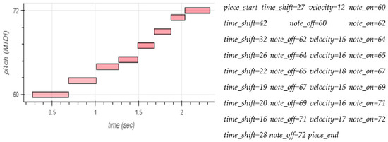
Figure 1.
Plot of a C major scale followed by its tokenized sequence. Note: On the left, we visualize the performance of a scale in C major in a two-dimensional plot of note (pitch) as a function of time (piano roll). On the right, we can see the token representation of this performance.
Intensity Quantization
The intensity (“velocity”) of a note is perceived as how loud or soft the note must be articulated. The common notation adopted in classical music has 8 levels of dynamic marking, ranging from ppp (pianissimo) to fff (fortissimo). However, the intensity component of the MIDI protocol has 128 levels of variation, ranging from 0 to 127.
The strategy adopted by Oore et al. [9] and later replicated by Cheng-Zhi et al. [12] was to quantize the 128 possible MIDI intensity levels into 32 “bins”. Considering that the original classical music notation has 8 levels of variation, 32 levels would be enough to reduce the sparsity of the model, leading to the intensity component being represented within a smaller space.
Quantization of Time Shifts
Time shift events are calculated as the difference between the temporal distance from the end of a note to the beginning of the next note in the sequence. The time difference calculation in its raw form takes place in a continuous space at the microsecond level. Thus, tokenizing the difference of all temporal possibilities would leave the model calculation unnecessarily sparse since, as noted by Friberg and Sundberg [13], the perceptible difference in the temporal displacement of a single tone in a sequence was not less than approximately 10 ms in average.
Because of this, to reduce the scope of temporal possibilities, each temporal displacement between one note and another was quantized in a range from 1 (10 ms) to 100 (1 s) in 10 ms increments. As a result, we obtained the space continuum quantization of the temporal displacement in a discrete space of 100 possibilities.
It is also noteworthy that the duration of the note was extended, referring to the fact that the piano pedal was considered in the total duration of the note.
Dataset Processing and Technologies Used
The tokenization process takes place in the entire augmented training and validation dataset, with a text file containing the concatenation of sequences of tokens as output.
The developed pre-processing structure is responsible for the acquisition and transformation of the MIDI dataset. The data acquisition part occurs through the download of the MAESTRO dataset [7]. As mentioned earlier, this dataset is a compilation of ten years of MIDI recordings from the international piano e-Competition. All performances were obtained through a Disklavier, which is a real piano with internal sensors that record MIDI events corresponding to the performer’s actions. The MIDI dataset files are organized by the performance competition year. The dataset also has a separation recommendation table for machine learning purposes, where each file is associated with a training, validation or test label.
The merging of validation data with training data was adopted as an approach, and thus, the test data was used for validation. In other words, the division between training, validation, and testing became training (old training + old validation) and validation (old testing). The choice of this approach came from the nature of the problem to be solved. Considering that the purpose of this work was to achieve the generation of musical sequences through a causal language model, the test division used in the traditional way did not add much value, considering that its practical application would be extremely similar to the validation division. Therefore, the adopted approach expanded the size of the training dataset, with the aim of giving the model more data.
The entire process of data acquisition and organization into training and validation took place in an automated way using bash and Python scripts. With the MIDI files organized, the transformation process could begin.
The transformation process took place in the following sequence for each MIDI file:
- Applying “sustain” pedal controls, extending the duration of each note according to the pedal dynamics used.
- Synthetic data augmentation using temporal transposition, “stretching” the time by ±25% and ±50%, resulting in 4 new examples plus the original.
- Synthetic data augmentation using pitch transposition in all intervals up and down by up to 6 semitones, resulting in 11 new examples plus the original.
- Extracting and transforming MIDI events and text strings.
Each MIDI file (followed by its respective synthetic data) was transformed into a textual sequence. Each textual string was added as a line in the text file relative to its grouping (training or validation). The result of the preprocessing was the transformation of all the MIDI files into two text files: data_train.txt and data_validation.txt. Their sizes were, respectively, 18 GB and 2.1 GB after preprocessing all MAESTRO dataset files. The entire data transformation process took place in an automated manner using the Python programming language, combined with the note-seq and pandas libraries.
2.2. Models
This work used four different music generation models, two of which are based on a recurrent neural network architecture, namely, long short-term memory (LSTM) models [14] and gated recurrent unit models [15]. The other two models were based on the transformer architecture [16]. Among the four models, three use pre-trained weights and one was trained from scratch through an end-to-end execution pipeline (from raw data to training). It is worth mentioning that a GPT2 model (Custom GPT2) was also trained in the same pipeline developed in this work. However, due to hardware limitations, the model did not converge to a significant result to the point of being considered for the blind test.
The reason for choosing this specific set of models came from the idea of comparing the musicality between prominent models, such as Music Transformers [10], MuseNet [17] and Performance RNN [9], from a human perspective. This choice also aimed to understand whether more complex pre-trained models, such as Music Transformers and its predecessor Performance RNN, would achieve a higher level of musicality than smaller models with similar architecture (Custom GPT2, Custom GRU). In this way, each model would represent a different type of musical quality.
Below, Table 1 shows the models that were applied during the research, along with their respective initial expectations of musicality.

Table 1.
List of models used in this research.
For the pre-trained models, transfer learning was used based on notoriously performant models available in each architecture [18]. For the long short-term memory architecture, the weights of the Performance RNN model presented by Oore et al. [9] were used. For the transformer-type models, the weights of the Music Transformers model implemented by Cheng-Zhi et al. [10] were used. The MuseNet model does not have either the code or the model weights open-sourced, but it has a web interface for music generation, which was used in this work. The choice of adopting pre-trained models came from the hardware limitation to achieve high-performance results given that training models of this nature are inherently complex from a computational perspective. The entire implementation of the models was carried out using the Python programming language combined with the Keras framework [19] with TensorFlow [20] and PyTorch [21]. HuggingFace ecosystem libraries, such as transformers [22], datasets [23] and tokenizers, were also used.
2.2.1. Framework for Music Generation with Performance RNN
Table 1 demonstrates that this model was expected to have high musicality due to its careful pre-training by Google researchers. However, its potential is limited compared with more advanced neural architectures, such as the ones utilized in transformers-based models, despite the potential improvement in quality that can be achieved through transfer learning.
The first step of this framework was to obtain the weights of the pre-trained model. As detailed bySimon and Oore [24], the weights of the models, as well as their source code, are made available by Google (the financier of the original research) through its Magenta repository on GitHub. The use of this model is linked to dependencies of other Python libraries, and thus, the creation of a virtual environment with all the necessary dependencies was found to be interesting for reproducibility purposes. The conda technology was used to create a virtual environment with all the necessary dependencies. Custom scripts for using and manipulating the model for MIDI generation were also developed in this work.
Finally, as a result of the sum of the aforementioned elements, we obtained the structure for generating MIDI files with the pre-trained Performance RNN model. The structure can be synthesized in the following steps:
- Obtaining the model weights and source code.
- Creation of a virtual environment for dependency resolution and reproducibility.
- Use of custom scripts to manipulate the model for MIDI generation.
2.2.2. Framework for Music Generation with Music Transformers
Similar to the Performance RNN model structure, the first step of the music generation structure with Music Transformers was to obtain the weights of the pre-trained model. Like the Performance RNN, the model’s source code is available in the Magenta repository from Google (who also funded the original research). However, the weights of this model are not as accessible as the Performance RNN. For the purpose of exemplifying the use of the model, Huang et al. [12] provided a jupyter notebook on the Google Colab platform. In this notebook, it can be identified that the model weights were downloaded through the gsutil tool, which enables access to Google’s internal Cloud storage. The tool is installed by default in the virtual environments created by Colab. Therefore, two ways of accessing the model weights were identified, as follows:
- Using gsutil on Google Colab followed by manual download. In this approach, the Colab environment is used to download the weights (Colab downloads from cloud storage). After downloading the weights in the Colab virtual environment, one can download the weights to the desired environment (client downloads from Colab).
- Use of the Google Cloud CLI tool in the desired environment. In this way, the desired environment has direct access to cloud storage without using the Colab platform.
The approach adopted was to use gsutil directly in the desired environment without the intermediary of Colab through the Google Cloud CLI tool. To facilitate the automation of the process, the docker tool was used together with the official Google Cloud CLI image to download the weights of the model. Scripts for automating this process were developed to facilitate reproducibility.
Similar to the Performance RNN model structure, Music Transformers also comes tied to a set of dependencies from other Python libraries. Therefore, the strategy of creating an adequate virtual environment was also applied in this case using conda technology. However, Music Transformers’ tensor2tensor dependency was “broken”, meaning that a piece of code needed to run the model was not working. After investigations into the reason for the problem, it was identified that the gym_utils.py file of the tensor2tensor library has an initialization problem in one of the parameters of its functions, where the kwargs parameter of the register_gym_env function was initialized with the value None. After removing this behavior, integration with the Music Transformers source code can be successful.
After adapting the dependencies, scripts for using and manipulating the model were developed to generate MIDI files. We can finally summarize the framework for music generation using Music Transformers in the following steps:
- Obtaining model weights through automation scripts using docker and Google Cloud CLI.
- Obtaining model source code from the Magenta repository on GitHub.
- Creating a virtual environment for dependency resolution and reproducibility.
- Suitability of dependencies (tensor2tensor) for functional integration with the model.
- Use of custom scripts to manipulate the model for MIDI generation.
The expected musicality of this model was very high given the complex nature of the model, which was based on the Transformers architecture. The fact that the model was carefully pre-trained by Google researchers also adds positively to the expected quality of this model. While this model may have been potentially robust, its expected performance could be limited in comparison to the MuseNet model, as it lacks the ability to generate by style and was trained on a smaller musical dataset.
2.2.3. Framework for Music Generation for the MuseNet Model
The source code and weights of the MuseNet model were not made publicly available by OpenAI, with all information pertinent to the development of the model limited to the article published on the company’s blog by Payne [17].
However, the published article provides an interface for interacting with the model, thus enabling musical generation with the model via the web. It is worth mentioning that the interface has some parameters to guide the musical generation, such as style (composition style), intro (input musical excerpt for conditional generation), and instruments. Aiming for homogeneity with the other models used, the style parameter was left with its default value of Chopin (classical pianist from the romantic period), intro was selected with the none option (start from scratch) for unconditional generation of tokens, and the parameter instruments was limited to piano. After adjusting the model parameters, tokens were interactively generated until a result lasting 30 s was obtained. After the musical generation, the interface offers the download of the created musical excerpt. This whole process can be summarized in the following steps:
- Access to the web interface of the MuseNet model provided by OpenAI.
- Model parameters adjustments.
- Generation of tokens in an iterative way, aiming to produce 30 s of music.
- Download the musical excerpt created by the model.
The quality expectation of this model was very high considering the architectural nature of its network (GPT-2 based) and its complexity, which shows the robustness of the results through a 72-layer network with 24 attention heads, expanding the scope of attention to a context of 4096 tokens. In addition, the extensive database used for training the model, added to the care of OpenAI researchers, supported the high expectation of quality. However, it is worth noting that experimentation with this model is the most limited among the tested models since their weights and source code were not made available by the company.
2.2.4. Training Framework and Music Generation for the Custom GRU and Custom GPT2 Model
The Custom GRU and Custom GPT2 models were completely developed and trained in this work. These models used the result of data pre-processing as the dataset, as detailed in Section 2.1.2.
It is worth noting that the Custom GPT2 model failed to achieve interesting results to be included in the blind test due to hardware limitations in view of the complexity of the model.
This section details the entire “pipeline” used for training music generation models.
Custom GRU
The Custom GRU model was developed with the aim to be an alternative to the Performance RNN model, comprising an architecture that was also based on recurrent neural networks. Unlike the Performance RNN model, which is based on layers of long short-term memory (LSTM [14]), the GRU model is based on layers of gated recurrent units [15]. The development of the model started from the work of Lee [25], which was built using the Python programming language combined with the PyTorch framework [21].
Table 2 below details the layers used in the model alongside their respective parameter quantities.
Table 2.
List of layers and parameters of neural networks in the Custom GRU model.
The model had 5,232,880 parameters in its entirety. All linear and embedding layers were initialized according to the method described by Glorot and Bengio [26] using a normal distribution. Therefore, the initial weights of the layers mentioned above were the result of the sampled values of N(0, std²), as defined in Equation (1):
where gain: optional scaling factor, number of layer inputs and : number of layer outputs.
On all initializations, gain assumed its default value of 1 (resulting in tensors not scaling). The model architecture started with a linear layer of 32 inputs and 1536 outputs, defined by Equation (2):
where x: layer input tensor, WT: layer weight transposed matrix and b: bias matrix.
The first linear layer was followed by an activation function of the hyperbolic tangent type, defined by Equation (3):
where x: output tensor of the previous layer.
The result of this activation function was then passed to an embedding layer of dimensionality [240 × 240]. The output of this layer was passed to another linear layer, followed by a leaky rectified linear unit (Leaky ReLU) activation function, defined by Equation (4):
where x: output tensor of the previous layer and : negative slope. The negative slope value used in this architecture was 0.1.
Then, the model followed with three layers of gated recurrent units [15], where each layer computed the system of equations, defined in Equation (5):
where reset port; : sigmoid function; , , and : learnable weight matrices and the bias vector for the reset port; : entry at time t; hidden state of the layer at time t − 1 or the initial hidden state at time 0; : update port; , , and : learnable weight matrices and the bias vector for the update port. new state port; , , and : learnable weight matrices and the bias vector for the new state port. *: Hadamard product; and : hidden state at time t.
Each gated recurrent unit layer had a total of 1,575,936 parameters, which were the sum of the layer’s hidden weights and biases. Finally, the model ended with a last linear layer followed by a softmax activation function to obtain the probability distribution of possible outcomes, defined by Equation (6):
where x: previous layer output tensor.
The loss function was defined with the cross-entropy calculation. The network backpropagation process was calculated with the Adam optimizer [27]. It is worth noting that gradient clip techniques were applied in the backpropagation process in an attempt to circumvent any explosive gradients. The technique basically consists of normalizing the gradient tensor in a range of −1 and 1 before performing the optimization with Adam.
The model was trained for 18 h on two 24 GB NVIDIA GeForce RTX 3090 GPUs with the following hyperparameters described in Table 3:
Table 3.
List of hyperparameters for training the Custom GRU model.
The model managed to reach a loss function value of 2.23 in the validation data. For the token generation, the model output was stochastically sampled using a beam search algorithm while the teacher forcing algorithm was applied to training. Although the architecture of this model was as robust as the pre-trained Performance RNN, its quality was expected to be lower given the limitation of the available hardware for its training.
Custom GPT2
The Custom GPT2 model was developed with the aim to be an alternative to the Music Transformers and MuseNet models. This model started from the implementation of a GPT2 causal language model [28] offered by the transformers library [22] through the HuggingFace platform.
- (1)
- Tokenizer
A “tokenizer” was trained to generate the vocabulary of the problem, using the pre-processed dataset of textual sequences as a base. The original tokenization training strategy of the GPT2 model [28] was based on the byte pair encoding (BPE) technique due to the extensive size of the worked vocabulary (50,257 tokens). Taking into account the fact that the data pre-processing strategy adopted in this work resulted in a relatively small vocabulary (390 tokens), the word level training technique was chosen for the tokenizer, which directly relates an identification number to each vocabulary token, thus making an event-to-token mapping. The HuggingFace tokenizers library was chosen to carry out this task due to its ease of manipulation and high performance.
- (2)
- Inputs and Model
The GPT2 model must receive a pre-defined tensor dimensionality for consistency of the matrix calculation in the input layer. The original implementation by Radford et al. (2019) uses sequences of 1024 tokens in “batches” of 512 sequences (input of [1024 × 512]). Unfortunately, these values could not be replicated due to a hardware limitation. Therefore, to adapt the model to the available hardware resources, sequences of 64 tokens in batches of 64 sequences were chosen (input of [64 × 64]). Sequences with more than 64 tokens were therefore truncated into multiple sequences less than or equal to 64 tokens, e.g., a sequence of 200 tokens [200 × 1] was transformed into four sequences of 64 [64 × 4]. It is worth noting in this example that the last sequence would initially have 8 tokens (200 = 64 + 64 + 64 + 8).
However, as mentioned earlier, the input tensor needs to have consistent dimensionality. Because of this, strings of tokens smaller than 64 had their difference in “PAD” tokens. “PAD” tokens are ignored by the model. Therefore, in the previous example, the last sequence of 8 tokens was extended with 56 “PAD” tokens, thus adapting the example tensor of [200 × 1] to a tensor of [64 × 4].
- (3)
- Training
The Custom GPT2 model managed to achieve a loss function value of 2.50 on the validation data after being trained for 116 h on two 24 GB NVIDIA GeForce RTX 3090 GPUs with the following hyperparameters listed in Table 4.
Table 4.
List of hyperparameters for training the Custom GPT2 model.
- (4)
- Detokonizer and Decoder
After training, the model was used to generate a musical language. Given one or more tokens in sequence and a maximum of M tokens to be generated, the GPT2 model output a sequence of dimensionality tokens [1 × M] in an autoregressive manner. The model outputs were stochastically sampled using the beam search technique, thus replicating the same strategy used in the Performance RNN, Music Transformers and Custom GRU models. From this point on, the data reverse engineering process could begin. The tokenizer was used in this step, but this time acting in the mapping of tokens to events, which were consequently processed via reverse engineering the techniques used in the pre-processing, obtaining a MIDI file as a result. However, the model was not able to converge in results interesting enough for the research, probably due to the complexity of the model faced by the limitation of available hardware.
2.3. Blind Test
The blind test was developed in three languages (Portuguese, English, and French) and was distributed through the SurveyMonkey online platform through three web forms (one for each language). For the blind test, three types of populations were initially selected:
- People who do not listen to classical music very often.
- People who listen to classical music often.
- Classically trained musicians.
The criterion adopted for choosing the aforementioned population was based on the hypothesis that musicians with a classical background and people who listen to classical music frequently have a greater ability to distinguish the compositional origin of a piece of music. The purpose of this criterion was to add details for the final analysis of the research.
All subjects had a total of five (number of generative models +1) musical excerpts to be heard, where one of them (+1) derived from a composition written by a human, randomly selected within the data used for training. A musical excerpt was collected from each model without any preconditioning. The musical excerpts were the same for the entire tested population, though they were initially ordered arbitrarily.
The following five questions were proposed for each musical excerpt:
- On a scale of 0 to 10, how musical do you think the piece of music heard is?
- ○
- Options from 0 to 10.
- Do you believe this song was made by a human or a computer?
- ○
- Binary Response (Human or Computer).
- Would you say that the musical excerpt heard resembles classical music?
- ○
- Binary Response (Yes or No).
- (Optional) Add any thoughts you might have about the excerpt heard.
- ○
- Free text.
It’s worth highlighting that some interesting answers of the optional free text question are listed on Appendix A.
After the end of the evaluations of the musical excerpts, the participants were directed to the following set of questions related to their musical experiences:
- How would you rate your musical sensitivity?
- ○
- Options from 0 to 10.
- How often do you listen to classical music?
- ○
- I don’t listen to classical music.
- ○
- Sometimes.
- ○
- Often.
- Do you have any practical experience with music?
- ○
- No.
- ○
- Yes, I can make music with my voice or a musical instrument.
- ○
- Yes, I study/I studied music theory (conservatory, music school, self-taught).
- ○
- Yes, I study/studied at a music university
The test consisted of a total of 23 questions, 20 (5 musical excerpts × 4) questions related to the musical excerpts heard and 3 questions related to musical experience.
3. Results
The blind test was performed by a total of 117 participants from different places around the world, including South America (Brazil), North America (USA and Canada) and Europe (France and Germany). The tested population was composed of professional musicians, music students at different levels (university and technical) and non-musicians. The test subjects were evaluated using three different spectra:
- Classical music consumption frequency.
- Musical experience.
- Musical sensitivity.
The evaluation metric for all populations was based on the success rate of questions 2, 6, 10, 14 and 18, which consisted of identifying the compositional origin of the excerpt heard. In other words, the metric was based on the average number of correct answers for the questions “Do you believe this song was made by a human or a computer?”.
3.1. Classical Music Consumption Frequency
Question 22 of the blind test featured the question “How often do you listen to classical music?”, with three possible answers, including “I don’t listen to classical music”, “Occasionally” and “I listen to it often”. Based on the answer to this question, the population was divided into three groups:
- Non-classical music listeners (31%).
- Casual classical music listeners (15%).
- Frequent listeners of classical music (54%).
The success rate of each group is illustrated in the graph shown in Figure 2.
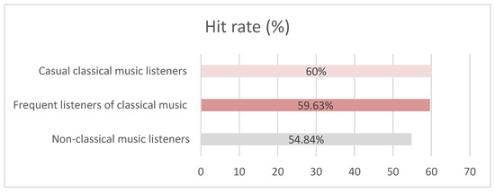
Figure 2.
Population hit rate averages across the frequency spectrum of consumption of classical music.
It can be seen from Figure 2 that casual and frequent listeners of classical music were more assertive in identifying the compositional origin of the musical excerpt heard than non-classical music listeners.
3.2. Music Experience
In this evaluation, the population was grouped by the spectrum of musical experience based on the answers to question 23 of the blind test “Do you have any practical experience with music?” The population was divided into the following groups:
- People with no music experience.
- Musicians.
- Musicians with knowledge of music theory.
- Musicians with advanced knowledge of music theory.
The average hit rate for each group can be seen in Figure 3.
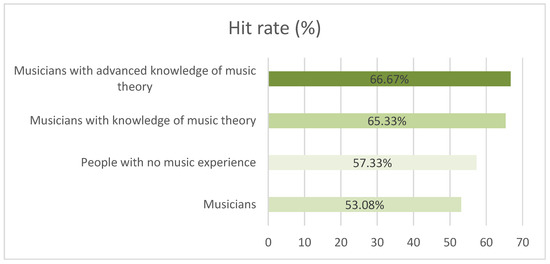
Figure 3.
Population hit rate averages across the musical experience spectrum.
It can be observed in Figure 3 that musicians with knowledge of music theory were more assertive in identifying the compositional origin of the musical passage heard than people with no experience in music theory.
3.3. Musical Sensitivity
The assessment of musical sensitivity was based on the answers to question 21 of the blind test: “How would you rate your musical sensitivity?”, where each test subject made a self-assessment of their musical sensitivity on a scale from 0 to 10, where 0 was described as “I cannot distinguish musical elements when I listen to music”, 5 as “I can distinguish certain musical elements, such as voice and instruments, when listening to music” and 10 as “I can perceive details of harmonic and melodic structure when I listen to music”.
The population was grouped using the following filters:
- People with high musical sensitivity (self-assessment > 7).
- People with average musical sensitivity (3 < self-assessment ≤ 7).
- People with low musical sensitivity (self-assessment ≤ 3).
The average hit rate for each group can be seen below in Figure 4.
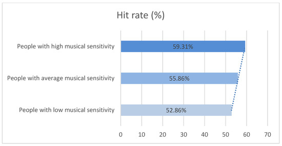
Figure 4.
Population hit rate averages across the musical sensitivity spectrum.
As illustrated by Figure 4, there was a linear relationship between musical sensitivity and the hit rate of the tested population, thus demonstrating that within the population tested, people with greater musical sensitivity were more assertive in identifying the excerpts heard.
3.4. Model Comparison
Data on the approval and evaluation of the musical excerpts heard was also collected during the analysis of each excerpt, which brought interesting insights. One of the perspectives to evaluate the musical quality of each passage was to look at the data by calculating the averages grouped by model, referring to the questions 1, 5, 9, 13 and 17 (“On a scale of 0 to 10, how musical do you think this song is?”).
It is interesting to observe in Figure 5 that, within the population tested, the MuseNet and Music Transformers models were better evaluated than the musical excerpt of human origin, randomly extracted from the MAESTRO dataset. It is also interesting to note that the models based on an RNN (Performance RNN and Custom GRU) were evaluated as less musical than those of human origin. Another perspective that is worth analyzing started with the evaluation of the compositional origin using the composer model, where we can observe the judgment of the tested population about the origin of the musical excerpt heard.
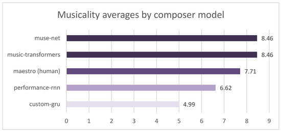
Figure 5.
Musicality averages by composer model.
As represented in Figure 6, the MuseNet model stood out once again, and by a slight margin of difference, the model was interpreted as being human more often than the genuinely human one. It is also worth highlighting that the musical excerpts derived from transformer architectures (Music Transformer and MuseNet) were able to confuse more than half of the population, which, in turn, was able to assertively distinguish the compositional origin of models based on an RNN (PerformanceRNN and Custom GRU).
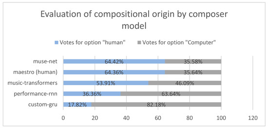
Figure 6.
Evaluation of compositional origin by composer model.
As a final point of view, illustrated in Figure 7, we analyzed the approval of musical excerpts as classical music grouped by model, that is, how many people voted “Yes” or “No” for questions such as “Would you say that the musical excerpt heard resembles music of the genre classic?”.
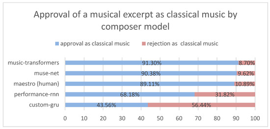
Figure 7.
Approval of a musical excerpt as classical music by composer model.
4. Discussion
The results of the blind test show the musical quality of the models based on transformer architectures, which, for the most part, surpassed the results of music of human origin. The results also demonstrate that models based on RNN architectures failed to achieve results that surpassed the results of the musicality of human origin. Furthermore, it can be seen that within the tested population, people with more experience in music theory, people who listen to classical music and people with greater musical sensitivity stood out in identifying when the musical excerpts were derived from an AI model and when they were derived from humans, thus corroborating the idea that people with more musical familiarity have a more assertive perception of the intrinsic details that distinguish a song composed by a machine from a song composed by a human. However, when analyzing the test results, it is important to consider various factors that may have influenced the outcome. For instance, differences in age, gender, education level, culture or other personal characteristics between the different groups could impact their cognitive abilities, attention span or familiarity with the testing procedures.
It is noteworthy to point out that within the gathered sample, the occasional listeners of classical music had a higher hit rate than frequent listeners of classical music. It is possible that differences in their exposure to classical music could have contributed to the differences in their average hit rate.
There is also the possibility that the test may have exhibited a bias toward specific categories of listeners. The given test structure may have favored occasional listeners who had more experience with practical classical music than frequent listeners who did not.
Another intriguing point to consider is the scenario in which individuals with no background in music achieved a higher success rate compared with musicians lacking theoretical knowledge. Some factors may contribute to the result, e.g., musicians with a familiarity with a specific musical genre other than classical, the lack of exposure to classical music composers or the used testing methods.
The sample size can have a significant impact on the aforementioned cases too, as the group sizes were imbalanced. In the scenario where people with no music experience (45 people) had a higher hit rate than musicians in a smaller sample (26 people), it is possible that the smaller sample size of musicians was not representative of the broader population of musicians and that this may have contributed to the differences observed in the hit rate between the two groups. The same logic can be applied to the comparison of the results between frequent listeners (54 people) and occasional listeners (15 people).
Overall, interpreting the test results can be complex and requires careful consideration of various factors that may have contributed to differences between the groups. Future research could aim to better understand the specific factors that influence cognitive performance in different musical contexts and to develop more targeted testing protocols that account for individual differences in musical experience and expertise.
5. Conclusions
This research presented an evaluation of symbolic music generative models from a human perspective through a blind test available online. This work also detailed possible pipeline development approaches for music generation through AI, in addition to demonstrating how to use transfer learning to generate music with pre-trained models.
In addition, the results of the blind test brought interesting insights into the musicality of the tested models, demonstrating that the musical excerpts derived from models based on transformers were the best evaluated, consistently surpassing, from different perspectives, results of human musical excerpts. Insights about the population were also presented, corroborating the understanding that within the tested population, people with more experience in music theory, people who listened to classical music and people with greater musical sensitivity were more able to correctly distinguish whether the musical excerpt was composed by a human or an AI. In conclusion, this study provides valuable insights into the human evaluation of a symbolic music generation models. However, it is important to acknowledge the limitations of this work, including the imbalanced sample size and limited musical genre used in the blind test. Future research should aim to address these limitations and expand the scope of inquiry to a broader range of musical contexts. Additionally, we suggest that future research should focus on developing more targeted testing protocols that account for individual differences in musical experience and expertise, and better understand the specific factors that influence cognitive performance in different musical contexts. By advancing our understanding of these factors, we can further explore the potential of generative models for music generation and advance the field of artificial intelligence in music.
Author Contributions
Conceptualization, P.F. and R.L.; Methodology, P.F. and R.L.; Software, P.F.; Validation, P.F.; Formal analysis, P.F.; Investigation, P.F.; Resources, P.F.; Data curation, P.F. and R.L.; Writing—original draft, P.F.; Writing—review & editing, P.F., R.L. and L.P.F.; Visualization, P.F. and R.L.; Supervision, P.F., R.L. and L.P.F.; Project administration, P.F., R.L. and L.P.F.; Funding acquisition, P.F. All authors have read and agreed to the published version of the manuscript.
Funding
The publication of this research was funded by Beslogic—Montreal, Canada (Grant Number 2023-02).
Informed Consent Statement
Informed consent was obtained from all subjects involved in the study.
Data Availability Statement
The data and the source code is available in a publicly accessible repository. The data presented in this study alongside with the source code of this research are openly available in Github, respectively at https://github.com/p-ferreira/generating-music-with-data/blob/main/test-results/all_responses.csv and https://github.com/p-ferreira/generating-music-with-data/ (accessed on 28 March 2023).
Conflicts of Interest
The authors declare no conflict of interest.
Appendix A
Below are some interesting comments collected from the research on the musical excerpts generated by the artificial intelligence models:
“It brings calm to my thoughts, I think of positive things and solutions for something I don’t know what it is”
Classical music listener of a musical excerpt from the Music Transformers model.
“The rests on lower notes make the melody more harmonious and more sentimental in this case.”
Musician with knowledge in music theory on an excerpt from the Performance RNN model.
“Perfect timing in cross voices, no delay time, so beautiful mechanical polyphony.”
Musician on a musical excerpt from the MuseNet model.
“The excerpt is more like a practice of musical scales than a piece of music itself.”
Musician with knowledge in music theory on excerpts from the Custom GRU model.
“It kept the feeling, there was a sequence in the harmony and rhythm, bringing the same feeling to the end.”
Music teacher and professional musician on an excerpt from the Performance RNN model.
“I found it really similar to calm, perfectly sounding classical music.”
Frequent listener of classical music of an excerpt from the Music Transformers model.
References
- Adorno, T.W.; Gillespie, S. Music, language, and composition. Music. Q. 1993, 77, 401–414. [Google Scholar] [CrossRef]
- Walder, C. Modeling symbolic music: Beyond the piano roll. In Proceedings of the Asian Conference on Machine Learning, Hamilton, New Zealand, 16–18 November 2016; pp. 174–189. [Google Scholar]
- Patel, A.D. Music, Language, and the Brain; Oxford University Press: Oxford, UK, 2010. [Google Scholar]
- Graves, A. Generating sequences with recurrent neural networks. arXiv 2013, arXiv:1308.0850. [Google Scholar]
- Mathews, A.; Xie, L.; He, X. Senticap: Generating image descriptions with sentiments. In Proceedings of the AAAI Con-ference on Artificial Intelligence, Phoenix, AZ, USA, 12–17 February 2016; Volume 30. No. 1. [Google Scholar]
- Loy, G. Musicians make a standard: The MIDI phenomenon. Comput. Music J. 1985, 9, 8–26. [Google Scholar] [CrossRef]
- Hawthorne, C.; Stasyuk, A.; Roberts, A.; Simon, I.; Huang, C.Z.A.; Dieleman, S.; Elsen, E.; Engel, J.; Eck, D. Enabling factorized piano music modeling and generation with the MAESTRO dataset. arXiv 2018, arXiv:1810.12247. [Google Scholar]
- Boulanger-Lewandowski, N.; Bengio, Y.; Vincent, P. Modeling temporal dependencies in high-dimensional sequences: Application to polyphonic music generation and transcription. arXiv 2012, arXiv:1206.6392. [Google Scholar]
- Oore, S.; Simon, I.; Dieleman, S.; Eck, D.; Simonyan, K. This time with feeling: Learning expressive musical performance. Neural Computing and Applications. arXiv 2018, arXiv:1808.03715. [Google Scholar]
- Huang, C.Z.A.; Vaswani, A.; Uszkoreit, J.; Shazeer, N.; Simon, I.; Hawthorne, C.; Dai, A.M.; Hoffman, M.D.; Dinculescu, M.; Eck, D. Music transformer. arXiv 2018, arXiv:1809.04281. [Google Scholar]
- Ens, J.; Pasquier, P. Mmm: Exploring conditional multi-track music generation with the transformer. arXiv 2020, arXiv:2008.06048. [Google Scholar]
- Huang, C.Z.A.; Simon, I.; Dinculescu, M. Music Transformer: Generating Music with Long-Term Structure. 2019. Available online: https://magenta.tensorflow.org/music-transformer (accessed on 4 February 2023).
- Friberg, A.; Sundberg, J. Perception of just-noticeable time displacement of a tone presented in a metrical sequence at different tempos. J. Acoust. Soc. Am. 1993, 94, 1859. [Google Scholar] [CrossRef]
- Yu, Y.; Si, X.; Hu, C.; Zhang, J. A review of recurrent neural networks: LSTM cells and network architectures. Neural Comput. 2019, 31, 1235–1270. [Google Scholar] [CrossRef] [PubMed]
- Cho, K.; Van Merriënboer, B.; Bahdanau, D.; Bengio, Y. On the properties of neural machine translation: Encoder-decoder approaches. arXiv 2014, arXiv:1409.1259. [Google Scholar]
- Vaswani, A.; Shazeer, N.; Parmar, N.; Uszkoreit, J.; Jones, L.; Gomez, A.N.; Kaiser, Ł.; Polosukhin, I. Attention is all you need. In Advances in Neural Information Processing Systems; MIT Press: Cambridge, MA, USA, 2017; Volume 30. [Google Scholar]
- Payne, C. Musenet. 2019. Available online: https://openai.com/blog/musenet (accessed on 4 February 2023).
- Ji, S.; Luo, J.; Yang, X. A comprehensive survey on deep music generation: Multi-level representations, algorithms, evaluations, and future directions. arXiv 2020, arXiv:2011.06801. [Google Scholar]
- Chollet, F. Keras. 2015. Available online: https://github.com/keras-team/keras (accessed on 4 February 2023).
- Abadi, M.; Agarwal, A.; Barham, P.; Brevdo, E.; Chen, Z.; Citro, C.; Corrado, G.; Davis, A.; Dean, J.; Devin, M.; et al. Tensorflow: Large-scale machine learning on heterogeneous distributed systems. arXiv 2016, arXiv:1603.04467. [Google Scholar]
- Paszke, A.; Gross, S.; Massa, F.; Lerer, A.; Bradbury, J.; Chanan, G.; Killeen, T.; Lin, Z.; Gimelshein, N.; Antiga, L.; et al. Pytorch: An imperative style, high-performance deep learning library. In Advances in Neural Information Processing Systems; MIT Press: Cambridge, MA, USA, 2019; Volume 32. [Google Scholar]
- Wolf, T.; Debut, L.; Sanh, V.; Chaumond, J.; Delangue, C.; Moi, A.; Cistac, P.; Rault, T.; Louf, R.; Funtowicz, M.; et al. Huggingface’s transformers: State-of-the-art natural language processing. arXiv 2019, arXiv:1910.03771. [Google Scholar]
- Lhoest, Q.; del Moral, A.; Jernite, Y.; Thakur, A.; von Platen, P.; Patil, S.; Chaumond, J.; Drame, M.; Plu, J.; Tunstall, L.; et al. Datasets: A Community Library for Natural Language Processing. arXiv 2021, arXiv:2109.02846. [Google Scholar]
- Simon, I.; Oore, S. Performance RNN: Generating Music with Expressive Timing and Dynamics. 2017. Available online: https://magenta.tensorflow.org/performance-rnn (accessed on 4 February 2023).
- Lee, Y. PyTorch implementation of Performance RNN, Inspired by Ian Simon and Sageev Oore. “Performance RNN: Generating Music with Expressive Timing and Dynamics. Magenta Blog. 2017. Available online: https://github.com/djosix/Performance-RNN-PyTorch (accessed on 4 February 2023).
- Glorot, X.; Bengio, Y. Understanding the difficulty of training deep feedforward neural networks. In Proceedings of the Thir-teenth International Conference on Artificial Intelligence and Statistics, JMLR Workshop and Conference Proceedings, Sardinia, Italy, 13–15 May 2010; pp. 249–256. [Google Scholar]
- Kingma, D.P.; Ba, J. Adam: A method for stochastic optimization. arXiv 2014, arXiv:1412.6980. [Google Scholar]
- Radford, A.; Wu, J.; Child, R.; Luan, D.; Amodei, D.; Sutskever, I. Language models are unsupervised multitask learners. OpenAI Blog 2019, 1, 9. [Google Scholar]


Disclaimer/Publisher’s Note: The statements, opinions and data contained in all publications are solely those of the individual author(s) and contributor(s) and not of MDPI and/or the editor(s). MDPI and/or the editor(s) disclaim responsibility for any injury to people or property resulting from any ideas, methods, instructions or products referred to in the content. |
© 2023 by the authors. Licensee MDPI, Basel, Switzerland. This article is an open access article distributed under the terms and conditions of the Creative Commons Attribution (CC BY) license (https://creativecommons.org/licenses/by/4.0/).