Article

A Cognitive Environment Modeling Approach for Autonomous Vehicles: A Chinese Experience

1
Hubei Research Center for New Energy & Intelligent Connected Vehicle, Wuhan University of Technology, Wuhan 430070, China
2
Hubei Collaborative Innovation Center for Automotive Components Technology, Wuhan University of Technology, Wuhan 430070, China
3
Hubei Key Laboratory of Advanced Technology for Automotive Components, Wuhan University of Technology, Wuhan 430070, China
*
Author to whom correspondence should be addressed.
Appl. Sci. 2023, 13(6), 3984; https://doi.org/10.3390/app13063984
Submission received: 1 March 2023 / Revised: 19 March 2023 / Accepted: 19 March 2023 / Published: 21 March 2023

Abstract

:
Existing environment modeling approaches and trajectory planning approaches for intelligent vehicles are difficult to adapt to multiple scenarios, as scenarios are diverse and changeable, which may lead to potential risks. This work proposes a cognitive spatial–time environment modeling approach for autonomous vehicles, which models a multi-scenario-adapted spatial–time environment model from a cognitive perspective and transforms the scenario-based trajectory planning problem into a unified spatial–time planning problem. The commonality of multiple typical Chinese road scenarios is analyzed, and a unified spatial–time environment model for multi-scenario adaptation is defined and established. The adaptability and trajectory planning potential of the spatial–time environment model are analyzed, and the planning results are obtained through a hybrid A* algorithm. The simulation results show that the proposal is effective in blurring the boundary between scenarios, allowing a single planning approach to adapt to multiple scenarios and plan optimal trajectories (optimal in both path and speed domains) and introducing more flexibility to the planning.

1. Introduction

1.1. Background

In the last decade, autonomous driving technology has been widely used in various scenarios [1], such as autonomous sweepers, autonomous buses, autonomous express delivery, etc., aiming to make transportation safer, more convenient, cheaper, and more environmentally friendly [2]. Trajectory planning includes path planning and speed profile generation, an essential part of an autonomous driving system. The planned trajectory should be flexible, collision-free, efficient, and satisfying to multiple preferences [3]. However, it is difficult for a single-trajectory planning approach to adapt to multiple scenarios due to the diversity of scenarios and the variability of scenario features; and it is difficult in path–speed cooperative planning to use a hierarchical path-first architecture, which is prone to potential risks. To solve these problems, the multi-scenario adaptation environment modeling approach and the trajectory planning approach should be studied.

1.2. Related Works

Environment models are the basis for motion planning in autonomous driving systems. These models build digital environments that are responsible for environmental assessment and trajectory planning [3]. The most common environment modeling approaches are scenario-based, and the challenge of current research lies in the modeling of dynamic scenarios and the trajectory planning in various scenarios [4].
Environment models for dynamic scenarios: Two-dimensional occupancy grid maps are the most-used environment models [5]. The environment can be represented if all the objects in the environment are projected onto the map. Occupied grids represent areas that should not be moved into, and free grids represent passable areas [6]. Moreover, the occupancy grid maps can overlay multiple 2D occupancy grid maps to represent environmental information, such as passable areas, potential collision risks, potential safe fields, and driving preferences [7]. These occupancy grid maps are widely used in robot path planning [8], but it is challenging to be compatible with autonomous vehicle trajectory planning in dynamic scenarios. In these cases, dynamic occupancy grid maps are proposed to handle dynamic scenarios [9]. Basically, a typical dynamic occupancy grid map is an occupancy map with multiple overlays of different times, which can represent the movement of environmental objects. There are other types of environment models. The Voronoi environment model [10] is proposed for non-structured roads with multiple static obstacles. However, it is challenging to introduce traffic rules. The weighted directed graph is a new solution for modeling and evaluation of structured road scenarios, which introduces multiple traffic rule constraints [11]. Some researchers have proposed the concept of continuous environmental models [12]. The list of obstacle information is a typical continuous environment model [13], which uses a sequence of locations with timestamps to represent all obstacles. It adapts to multidomain scenarios (structured roads, half-structured roads, and off-road), but it is challenging to introduce additional safety costs and requires a lot of computing power to get results.
Trajectory planning approaches in various scenarios: There are two architectures of trajectory approaches: hierarchical architecture and integrated architecture. (1) Most existing planning approaches are hierarchical architecture approaches. It is a brilliant idea to handle the task of autonomous vehicle motion planning as a classic hierarchical robot motion planning task [14]. The path and the speed profile are planned separately [15]. The speed profile is attached after the path is planned. This hierarchical architecture is functional in most scenarios, such as car following scenarios [16], lane changing scenarios [17], emergency stop scenarios, dynamic scenarios with few dynamic objects, and scenarios that can be converted into simple scenarios. The path can be generated through state–machine-based planners [15], lattice-based planners [18], RRT-based planners [19], A-star-based planners [20], Dijkstra-based planners [10], numerical-optimization-based planners [21], etc. Additionally, the speed profile can be generated by rule-based planners [15], S–T-graph-based planners [21], numerical-optimization-based planners [22], etc. (2) Integrated trajectory planners are functional in both common and “corner case” scenarios. Roundabout scenarios are typical “corner case” scenarios [23]. There are multiple cut-in and cut-out obstacles that affect the movement of the ego vehicle. Usually, reinforcement-learning-based approaches are applied to these scenarios instead of hierarchical approaches [24]. The unprotected left turn scenario is another typical “corner case” scenario [25], a multi-obstacle game scenario [26]. The multivehicle cooperative control scenario is also a corner case scenario that requires trajectory planning approaches to perform integrated planning of multivehicle motion trajectories [27]. It is difficult for feasible trajectories to be planned. In fact, the integrated trajectory planners bring higher flexibility and planning success rate in “corner case” scenarios, which is one of the current research hotspots.

1.3. Motivations and Contributions

The most common environment modeling approaches and trajectory planning approaches are scenario-based approaches that are difficult to adapt to multiple scenarios for the following reasons: (1) It is challenging to model multiple scenarios and complex dynamic scenarios using one environment model. In the existing approach, structured road scenarios, half-structured road scenarios, complex dynamic scenarios and other corner case scenarios are modeled using different environment models, which are difficult to model using normalized models. (2) It is challenging for single-trajectory planning approaches to adapt to multiple scenarios. Due to the difficulty in normalizing the modeling of each scenario, the trajectory planning approach is difficult to adapt to different scenarios, and different approaches have to be designed for different scenarios. (3) It is challenging for trajectory planning approaches to plan the optimal trajectories in path and speed domains using a traditional environment model. The most common planning approaches are hierarchical architectures with path-first and speed-later, which cannot achieve integrated path–speed planning, resulting in potential risks and no solution in some scenarios.
This work proposes a cognitive environment modeling approach using a spatial–time environment model. (1) A spatial–time environment model is constructed to normalize and discretize the variable scenarios, and the variable scenarios are transformed into a unified environment model of the X–Y spatial domain and the time domain, making it possible to normalize the modeling of multiple scenarios using one environment model. (2) The multi-scenario adaptation of the model is analyzed, providing the possibility for multi-scenario adaptation of a single-trajectory planning approach. (3) The integrated path–speed planning using a spatial–time model is analyzed and simulated. Together, this demonstrates the advancement of integrated planning.

1.4. Organization

The rest of this paper is structured as follows: In Section 2, a novel system architecture for autonomous vehicles is proposed. In Section 3, the modeling process for the spatial–time environment model is introduced. In Section 4, the scenario compatibility of the spatial–time environment model is analyzed. The trajectory planning approach compatibility of the spatial–time environment model is analyzed in Section 5, followed by concluding remarks in Section 6.

2. System Architecture

The system architecture of the spatial–time environment model approach is shown in Figure 1. It is a hierarchical architecture that takes perception results, localization information, and mission planning results as inputs, and outputs a spatial–time environment model to the planning module. There are two main steps in the architecture: static object (non-time-varying) discretization and dynamic object (time-varying) discretization.
Static object discretization refers to the projection of non-passable areas or various types of constraints into the spatial–time environment model. For example, the area occupied by static obstacles, the non-passable area with strong traffic constraints, the non-passable area introduced by additional constraints, etc. Dynamic object discretization refers to the projection of dynamic non-passable areas into the spatial–time environment model. For example, the occupancy relationship of dynamic obstacles to spatial–time, the occupancy relationship of traffic signals in spatial–time, etc. The results of static object discretization and dynamic object discretization together form the spatial–time environment model. This model can normalize various objects in the driving scenario and build a normalized and discrete environment model from the perspective of scenario cognition.
Thus, this cognitive spatial–time environment model has transformed the classical hierarchical architecture [15] of the trajectory planning problem into an all-in-one planning problem, where there will no longer be separate behavior planning and path planning modules. Spatial–time environment model-based trajectory planning offers the possibility to directly obtain the optimal trajectory (optimal in path and speed), where the optimal path and the optimal speed profile can be obtained by integrated planners, so that the optimal trajectory can be obtained. Spatial–time environment model-based trajectory planning provides the possibility of multi-scenario adaptation of a single-trajectory planning approach, as the variable scenarios are normalized by the spatial–time environment model into a cognitively unified model, without differentiation by scenario. The scenario-based trajectory planning problem has transformed into a unified planning problem for multi-scenario adaptation.

3. Spatial–Time Environment Model Statement

3.1. Definition

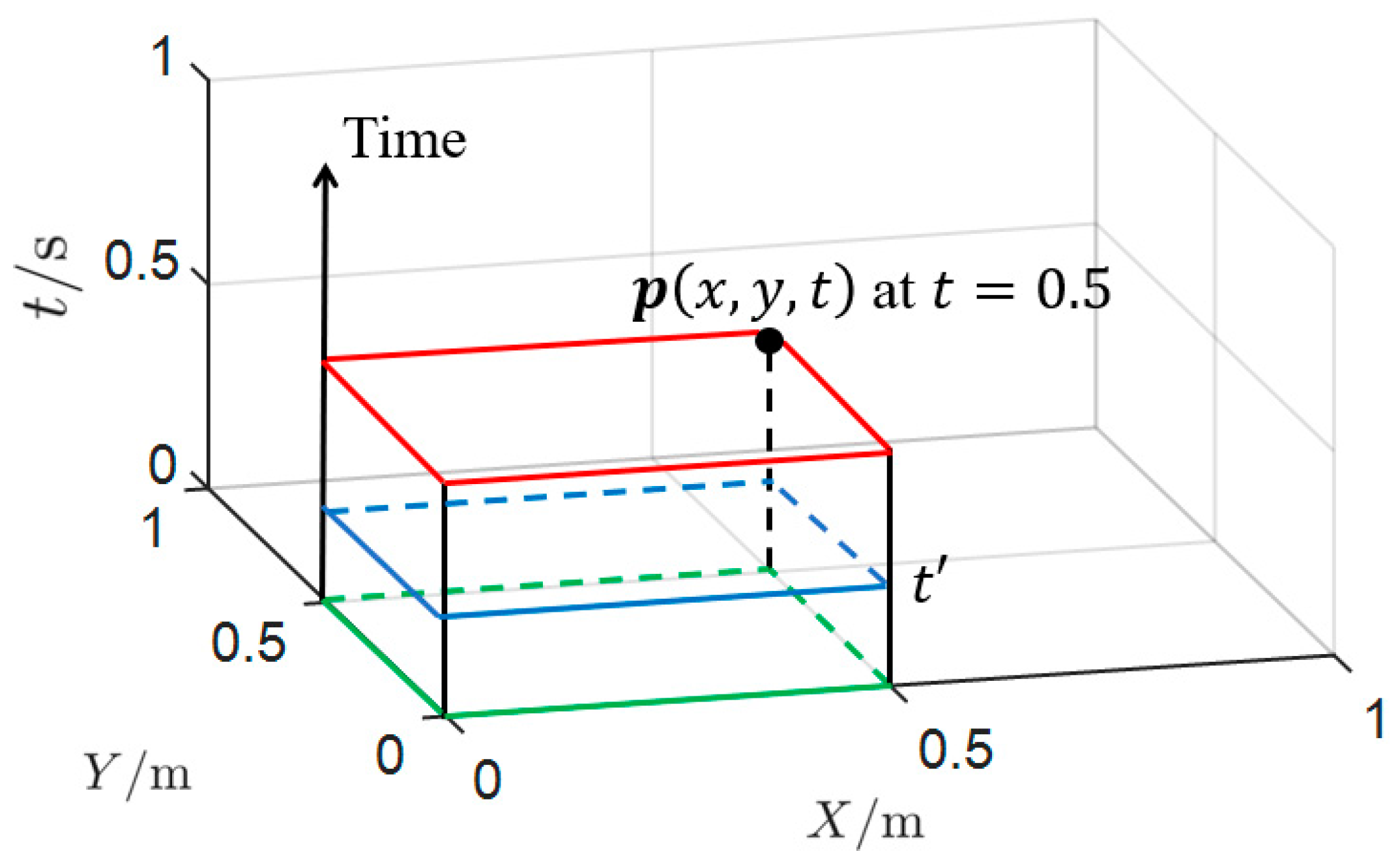
The spatial–time environment model is a 3D spatial–time occupancy grid map consisting of a series of 2D occupancy grid maps at different times t . In this work, we model the environment with a resolution D M = 0.1 per grid. An example spatial–time environment model M s t is shown in Figure 2, which contains three coordinate axes: the X axis, Y axis, and time axis. The X axis and the Y axis form a space plane (capable both in Gaussian coordinates and vehicle coordinates) at time t . The time axis represents the time during which the plane is located. The green-line plane in Figure 2 represents the 2D occupancy grid map at t = 0   s , which represents the occupancy in the region of interest on the road at the current moment t = 0   s (the plane where the autonomous vehicle is located), and the blue-line plane represents the 2D occupancy map at the time t . If the ego vehicle is at the origin of the coordinate system, p ( x , y , t ) is an occupied point located at X = 0.5   m , Y = 0.5   m that will appear after 0.5 s. The point p at time t = 0.5   s in the spatial–time domain is no longer a feasible driving region, as it is occupied, T ( p ) = 1 (0 for free). The ego vehicle should avoid this point at time t = 0.5   s .
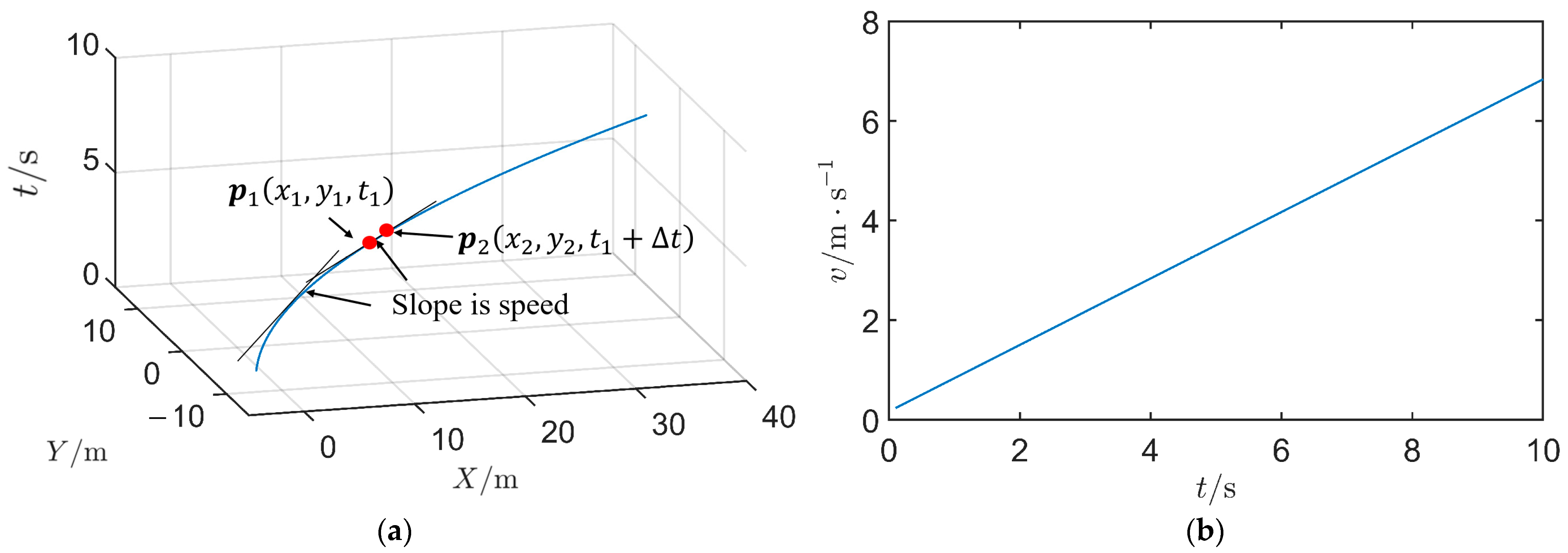
An example M s t is shown in Figure 3, which contains one dynamic time-varying obstacle. The moving speed of the obstacle in the spatial–time domain can be obtained by derivation. Assuming that p 1 ( x 1 , y 1 , t 1 ) and p 2 ( x 2 , y 2 , t + Δ t ) are two points at different times on a dynamic obstacle trajectory, where Δ t D M , the average moving speed between them can be calculated by
v ( p 1 , p 2 ) = l i m Δ t D M ( y 2 y 1 ) 2 + ( x 2 x 1 ) 2 Δ t

3.2. Static Object Discretization

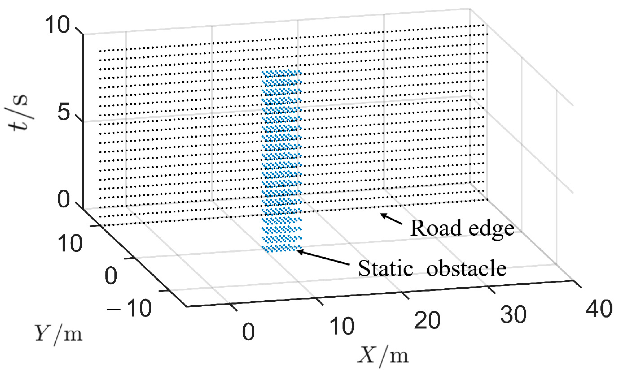
As shown in Figure 4. Static objects are objects whose position and shape do not change over time, including solid static objects and virtual static objects. (1) Solid static objects are real static obstacles in the environment, including static obstacles, road boundaries, driving area constraints, etc. (2) Virtual static objects usually are static constraints, such as additional environmental constraints (road edge, stop sign, parking gate, driving behavior preference, etc.). As Figure 4 shows, a time-invariant static object (blue dots) is projected onto the spatial–time environment model, and an example virtual obstacle (road edge, black dots) is also projected onto the spatial–time environment model. Their projections are time-invariant in the X–Y domain, occupying the corresponding locations from the start moment t 0 to the end moment t e n d of the spatial–time environment model.

3.3. Dynamic Object Discretization

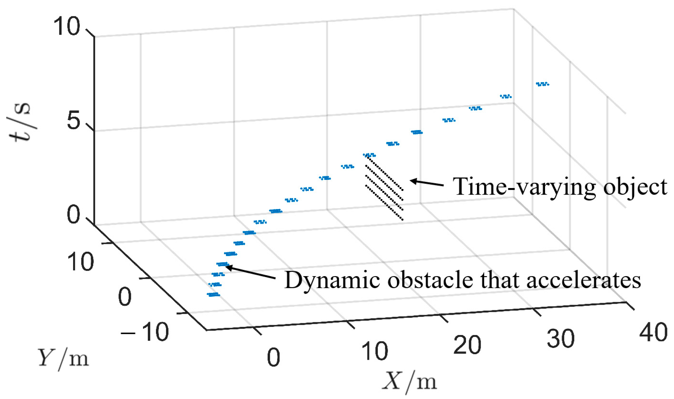
As shown in Figure 5. Dynamic object discretization is a process that projects time-varying objects onto the spatial–time environment model. Dynamic objects are objects whose position and shape change over time, including solid dynamic objects and virtual dynamic objects. (1) Solid dynamic objects are real dynamic objects in the environment, including dynamic obstacles and objects whose shape changes over time. An example of a dynamic obstacle is shown as the blue dots in Figure 5, which is an accelerating vehicle, represented as a curve in the spatial–time domain. Non-stationary objects such as moving vehicles and walking people are typical solid dynamic objects. (2) Virtual dynamic objects are time-varying but stationary objects that appear and disappear over time. An example of a time-varying virtual dynamic object is shown as the black dots in Figure 5. It appears at t = 2   s , and disappears after t = 3   s . Virtual dynamic objects include traffic lights, speed limit signs, etc.

3.4. Trajectory Planning Problem Statement in the Spatial–Time Environment Model

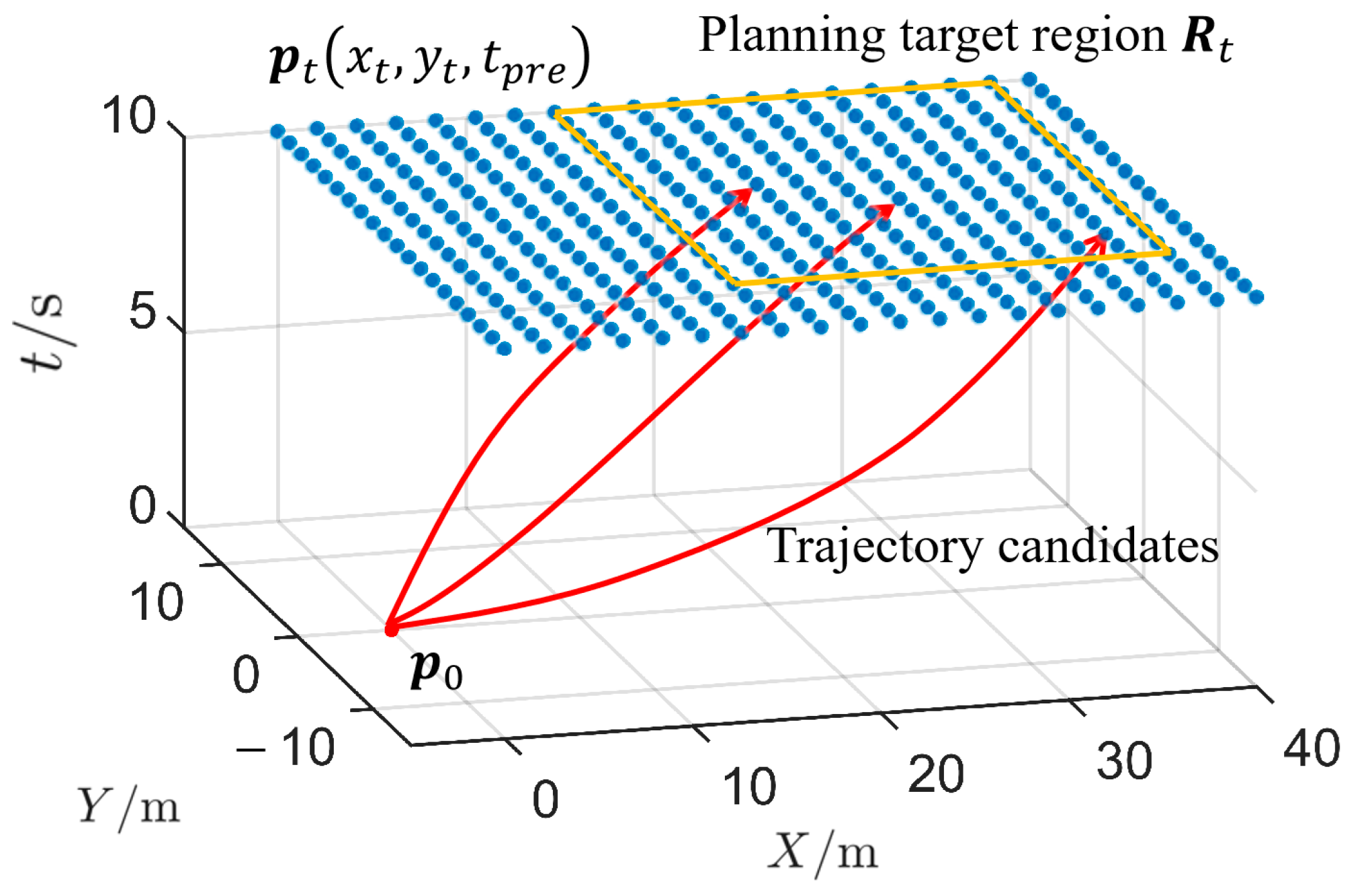
The trajectory planning problem is the problem of obtaining an optimal solution in the remaining feasible spatial–time area under multiple constraints. In fact, it is a spatial path planning problem under constraints, obtaining collision-free feasible trajectories connecting the start point p 0 and the target point p t . As shown in Figure 6. Three example trajectories are shown as the red lines in Figure 6, containing the motion of the vehicle in the X–Y domain and the speed profile in the X–Y–t domain. For example, if the trajectory for the next 10 s needs to be planned, the preview time can be set as t p r e = 10   s . It should be noted that the maximum value of X ( X m a x ) can be determined according to the maximum speed limit v m a x of the vehicle, X m a x p p r e × v m a x . The blue dots represent the target point candidates for t = t p r e in the X–Y domain. The dots within the planning target region R t marked by the yellow rectangle are the target points p t ( x t , y t , t p r e ) R t . Moreover, R t is a variable area; its size is adjusted in real-time as needed.

3.5. Collision Checking

Collision checking is a critical part of autonomous driving systems, detecting whether the planned trajectories collide with obstacles or not in space and time. Assuming that the spatial–time environment model is M s t , and the projection of one given trajectory P n ( n = 1 , 2 , 3 , , N ) is M t r a j n ( n = 1 , 2 , 3 , N ) .
I s C o l l i s i o n = { 0 ( M s t ° M t r a j N = 0 ) 1 ( M s t ° M t r a j N > 0 )
where ° is an operator that multiplies the objects at the corresponding in two matrices; X is an operation that sums the objects in matrix X ; and N is the number of trajectories.
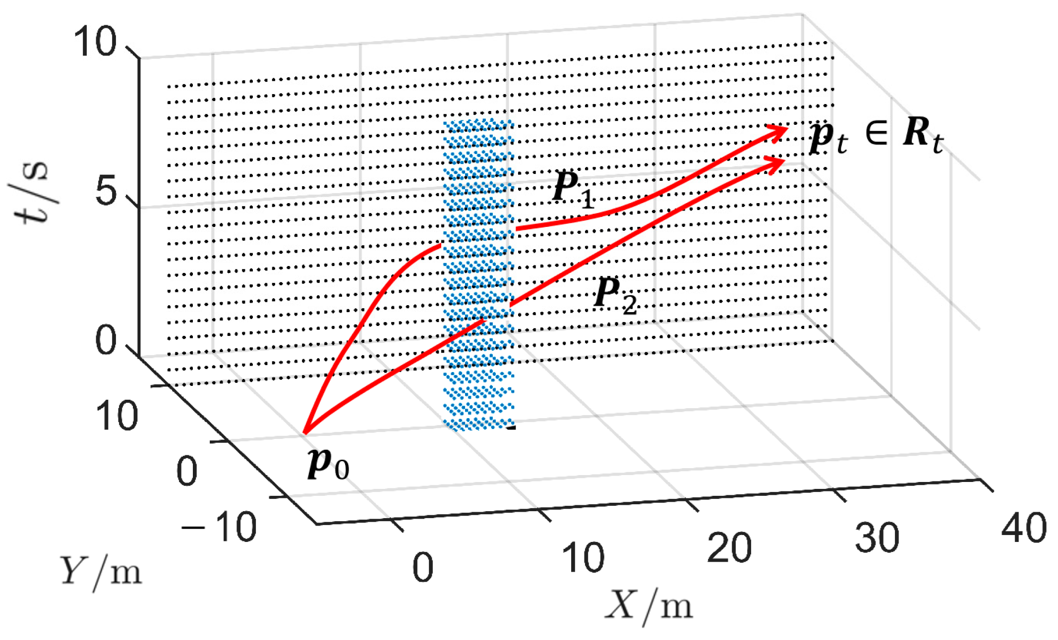
Figure 7 shows a typical collision checking scenario, where P 1 and P 2 represent two trajectories, and p 0 and p t represent the vehicle location at t 0 and the target point that the vehicle should move to. Obviously, M s t ° M t r a j 2 > 0 , indicating that P 2 is not a collision-free trajectory, and a collision occurs. M s t ° M t r a j 1 = 0 , indicating that P 1 is a feasible collision-free trajectory which passes through the gap between occupied grids.

3.6. Cost Assessment Model

The cost assessment model is functional for trajectory optimization. Multiple cost assessment indicators such as road cost, dynamic cost, kinematic cost, safety preference cost, and additional constraint costs need to be introduced. It provides the possibility for trajectory optimization.
An example cost assessment model at time t is shown in Figure 8, which is a road cost model using the cost assessment approach presented in paper [28]. If the cost matrix at time t can be represented by E c ( t ) , the cost information of one given trajectory at time t can be presented by M t r a j n ( n = 1 , 2 , 3 , , N ) . The cost E t r a j of one trajectory can be obtained. It is important to recall that this is a simple example of cost assessment, and a more detailed explanation will be shown in our following research paper on spatial–time environment model-based multiple scenario adaption trajectory planning.
E t r a j = t = 0 t = t p r e || E c ( t ) ° M t r a j N ||

4. Scenario Compatibility

The spatial–time environment model is compatible with multiple Chinese road scenarios, especially dynamic scenarios. To make the figures easier to understand, the spatial–time environment model in some scenarios only contains essential objects.

4.1. Static Obstacle Avoidance Scenario

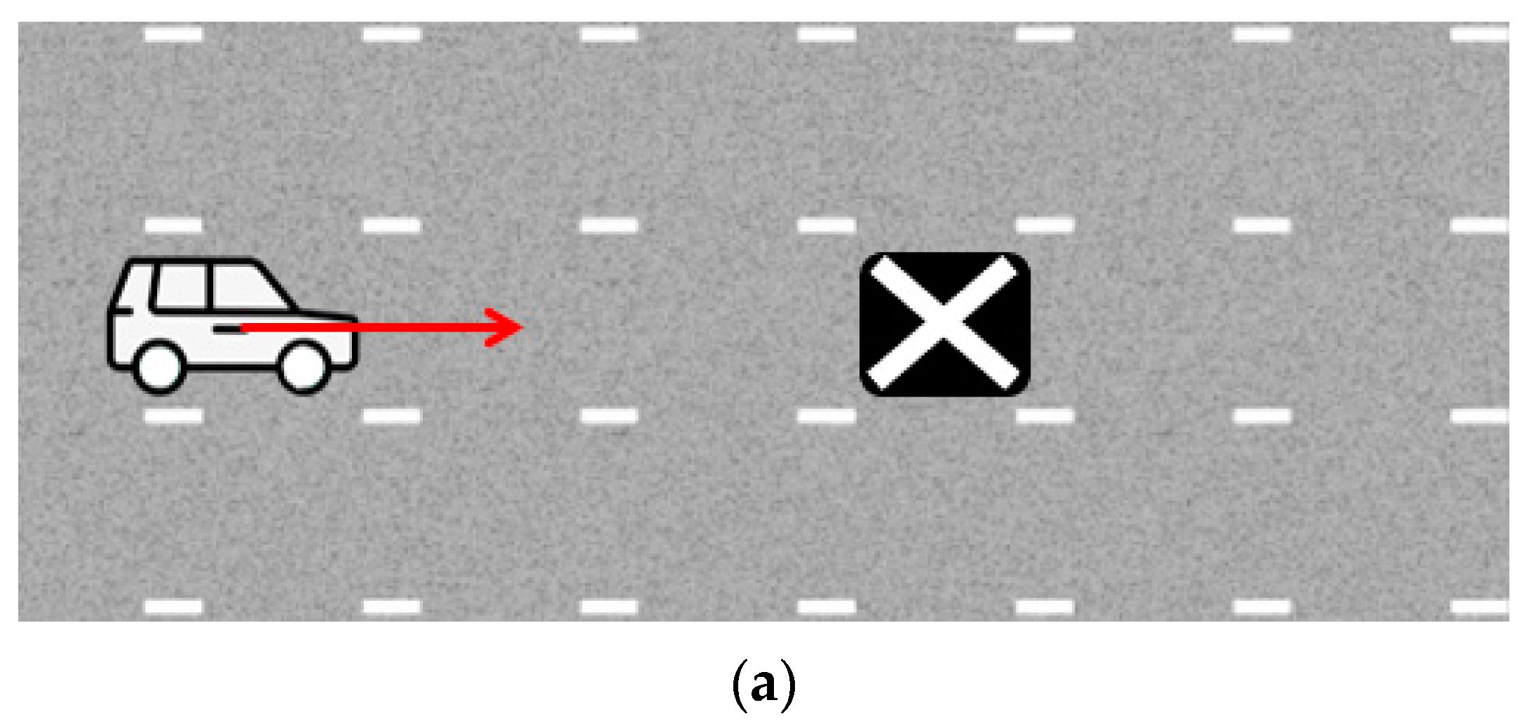
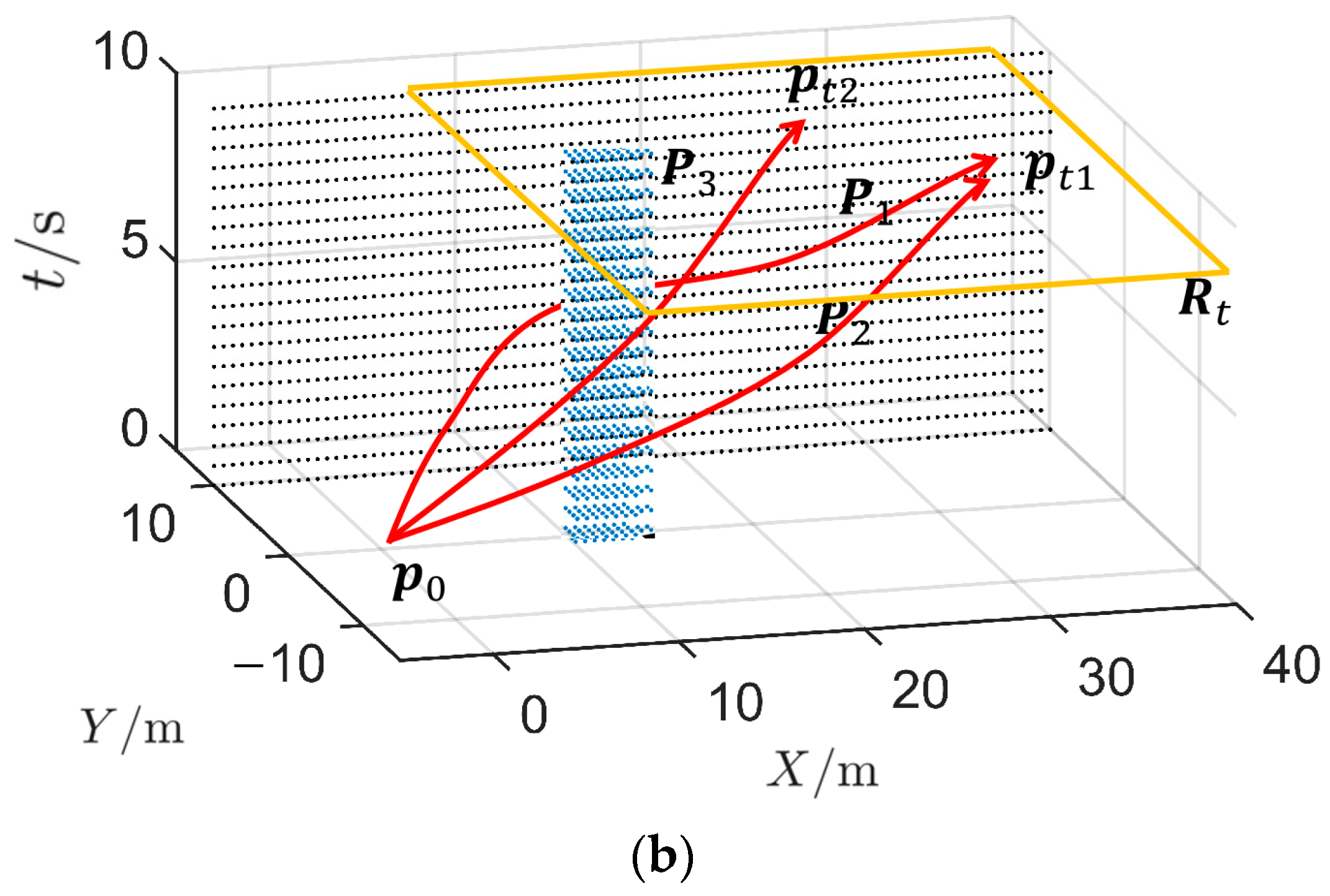
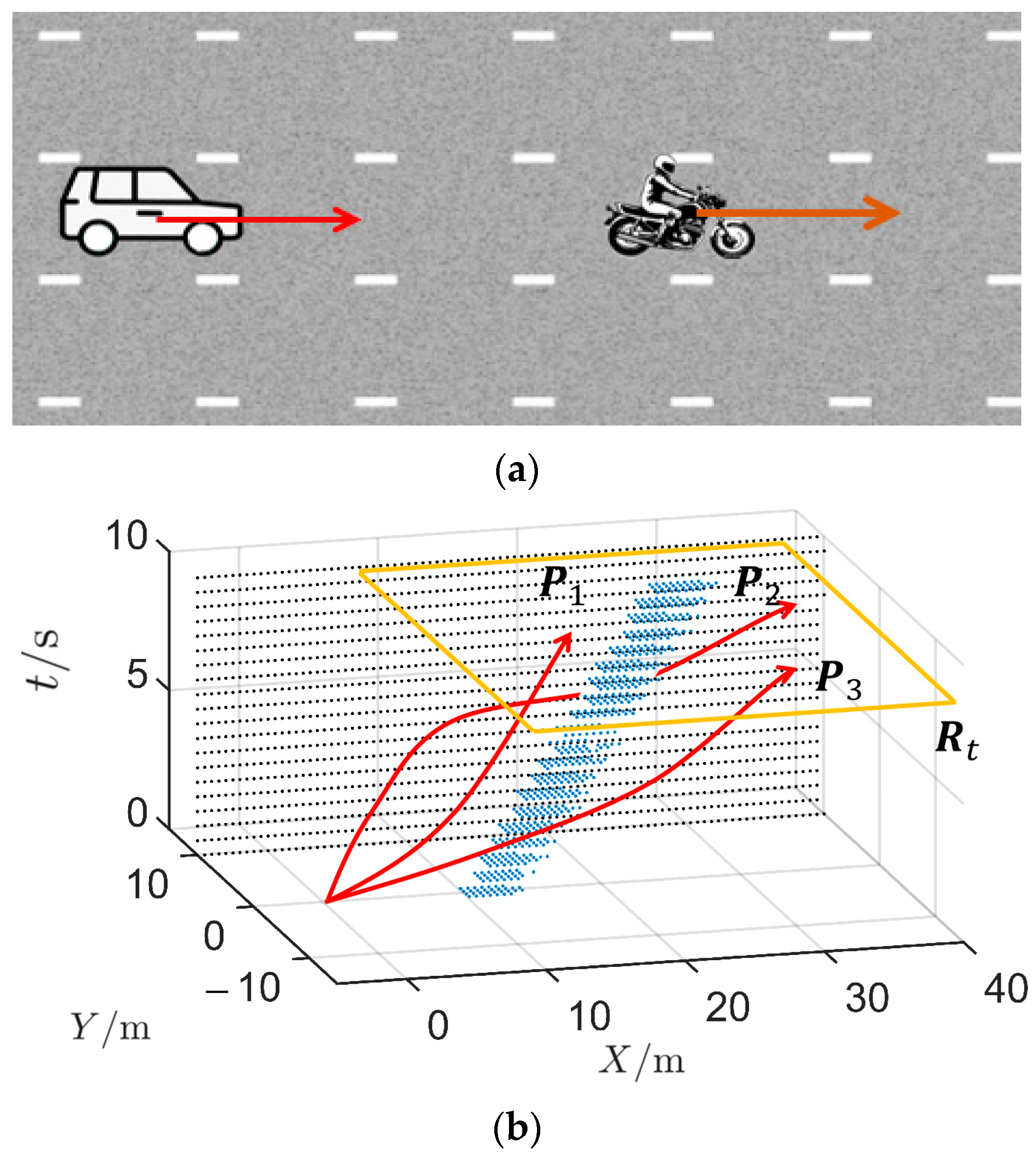
Static obstacle avoidance scenarios are the most common scenarios. Figure 9 shows an example static obstacle avoidance scenario, where P 1 , P 2 , and P 3 are different types of feasible trajectories; p 0 is the vehicle location at t 0 = 0   s ; and p t 1 and p t 2 are two points belonging to R t . There are three plans (three types of trajectories) to avoid the static obstacle. P 1 ( p 0 p t 1 ) is a trajectory that overtakes to the left. P 2 ( p 0 p t 1 ) is a right-overtaking trajectory with the same longitudinal speed as P 1 , but smoother in the X–Y domain. P 3 ( p 0 p t 2 ) is a trajectory that overtakes to the right at a lower speed than P 1 and P 2 .

4.2. Dynamic Overtaking Scenario

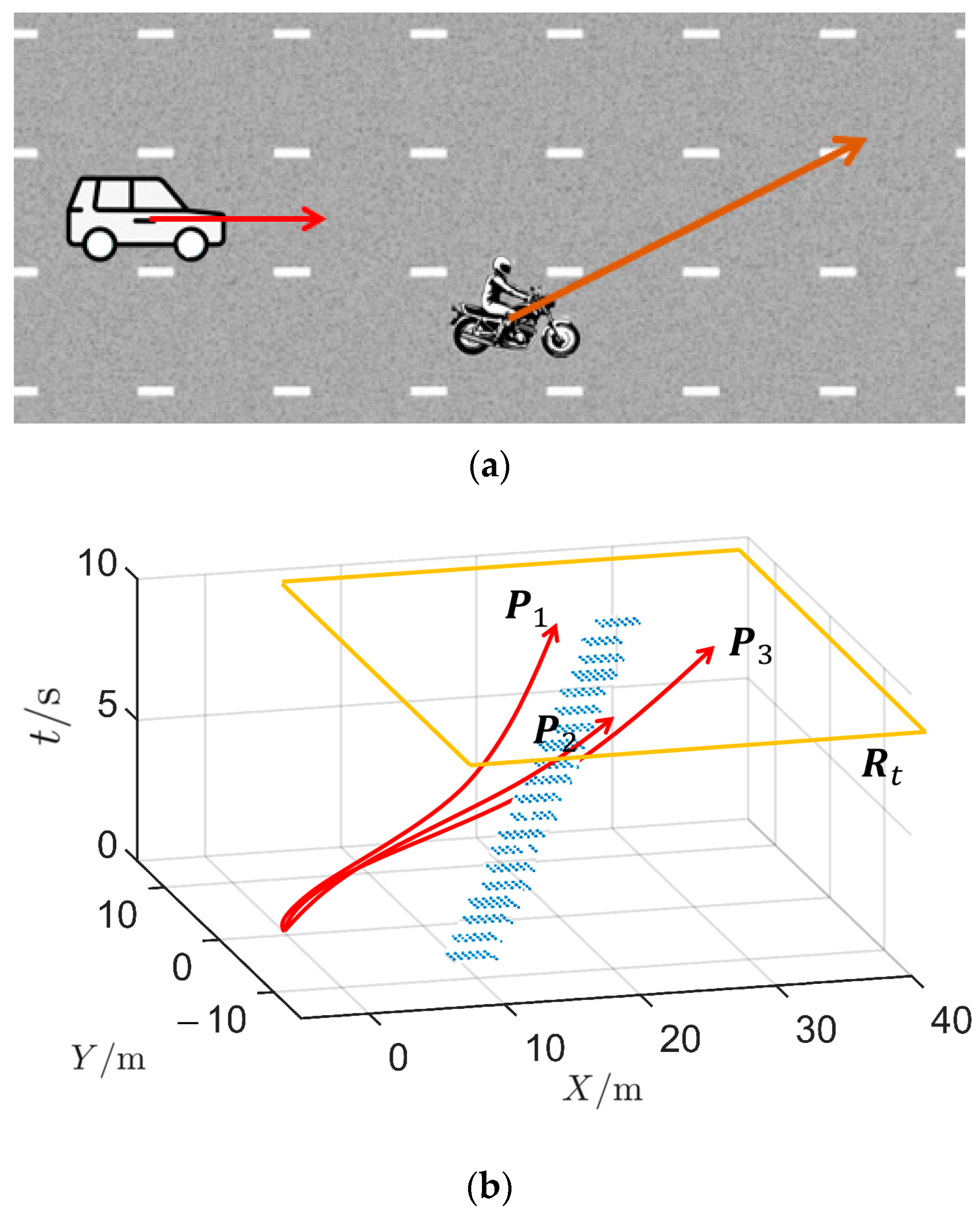
Dynamic overtaking scenarios are the most common dynamic obstacle avoidance scenarios. The dynamic obstacles to be overtaken are obstacles that affect the driving of the ego vehicle and move in the same direction as the ego vehicle. They can be active vehicles, bicycles, pedestrians, pets, etc. An example of a dynamic overtaking scenario is shown in Figure 10. A dynamic obstacle moves at a constant speed ahead of the ego vehicle. There are three plans for the ego vehicle to move: slowing down and following the dynamic obstacle, accelerating and overtaking the obstacle from the left, and changing lanes and overtaking the obstacle from the right. As shown in trajectory P 1 , the ego vehicle slows down and follows the obstacle. P 2 is a left-overtaking trajectory; the ego vehicle changes lanes to the left and then accelerates to overtake. P 3 is a right-overtaking trajectory; the ego vehicle changes lanes to the right and overtakes the dynamic obstacle.

4.3. Dynamic Cut-in Scenario

Figure 11 shows a cut-in scenario, where a vehicle cuts into the trajectory of the ego vehicle from right to left. The ego vehicle should change its state to avoid a potential collision. The spatial–time model provides three options for the vehicle to avoid potential collisions. P 1 is a collision-free trajectory; the ego vehicle decelerates to avoid the cut-in obstacle, and the obstacle will pass in front of the ego vehicle. P 2 is also a collision-free trajectory in which the ego vehicle avoids the obstacle to the right. P 3 is an active obstacle avoidance trajectory; the ego vehicle accelerates to overtake the obstacle before the obstacle cuts into the trajectory of the ego vehicle.

4.4. Lane Merging Scenario

An example lane merging scenario is shown in Figure 12. The ego vehicle will change lanes to the left, and there are two dynamic obstacles in the left lane. Three lane changing options are available. In P 1 the ego vehicle accelerates and changes lanes to the left, inserting itself between the two moving vehicles. In P 2 the vehicle merges to the left after a rapid accelerates and overtakes the two moving vehicles.

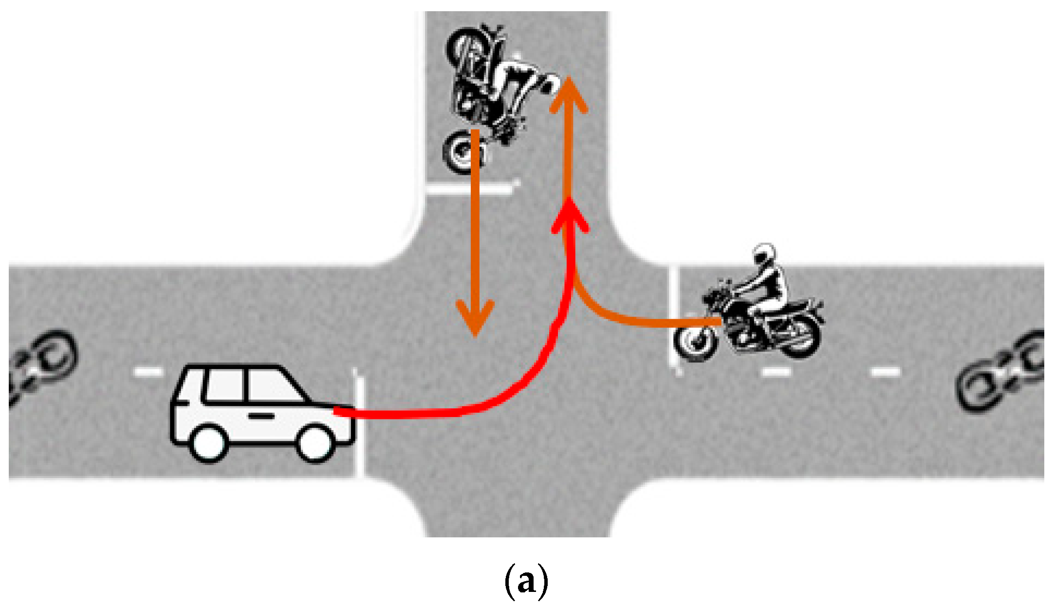
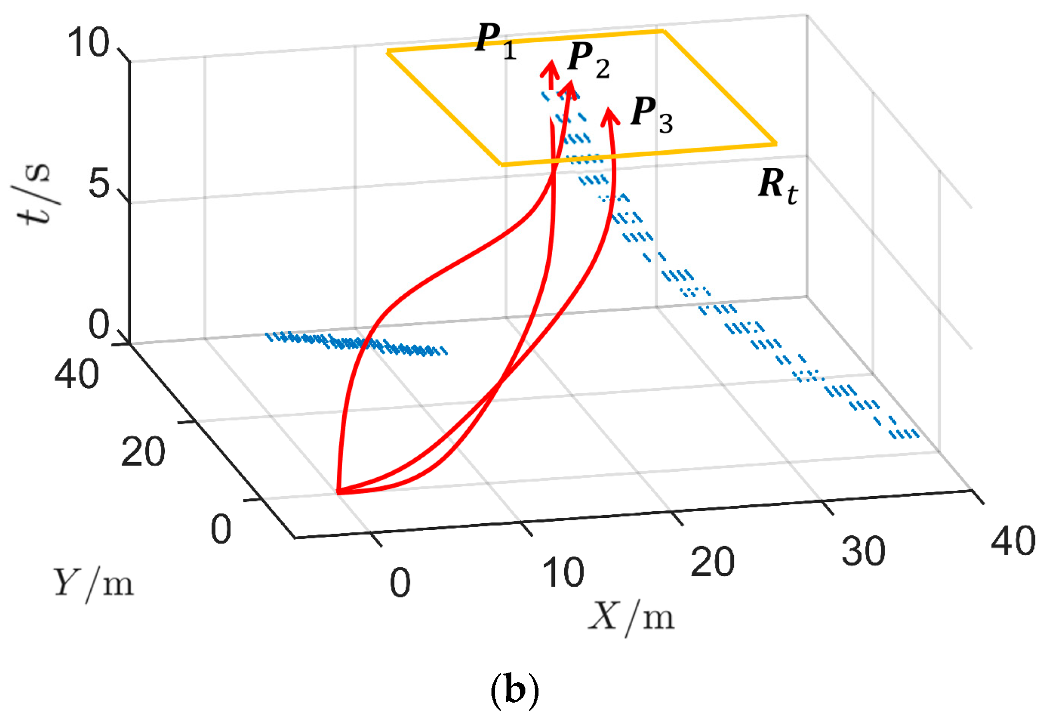
4.5. Unprotected Left Turns with Traffic

An example unprotected left turn with traffic scenario is shown in Figure 13. The ego vehicle should turn left and avoid dynamic obstacles. There are three trajectory options. In P 1 the vehicle accelerates and finishes the left turn before dynamic obstacles pose a threat. In P 2 the vehicle deaccelerates, waiting for one of the dynamic obstacles to pass, then the vehicle accelerates and turns left before the other dynamic obstacle poses a threat. In P 3 the vehicle accelerates to avoid the first dynamic obstacle, and then deaccelerates to wait for the second dynamic obstacle to pass.

4.6. Roundabout Scenario

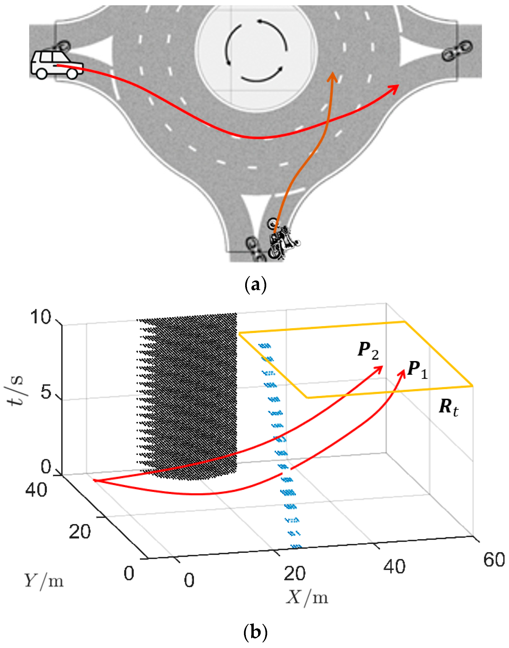
An example roundabout entry and exit scenario is shown in Figure 14. It is basically an unstructured road scenario where the vehicle needs to avoid obstacles without strictly complicated traffic rules. To that end, there are two typical options for the vehicle to drive. In P 1 the vehicle makes a quick pass, then accelerates and exits the roundabout before other dynamic obstacles hit it. In P 2 the vehicle passes slowly and bypasses the dynamic obstacle.

4.7. Traffic Light Traffic Scenario

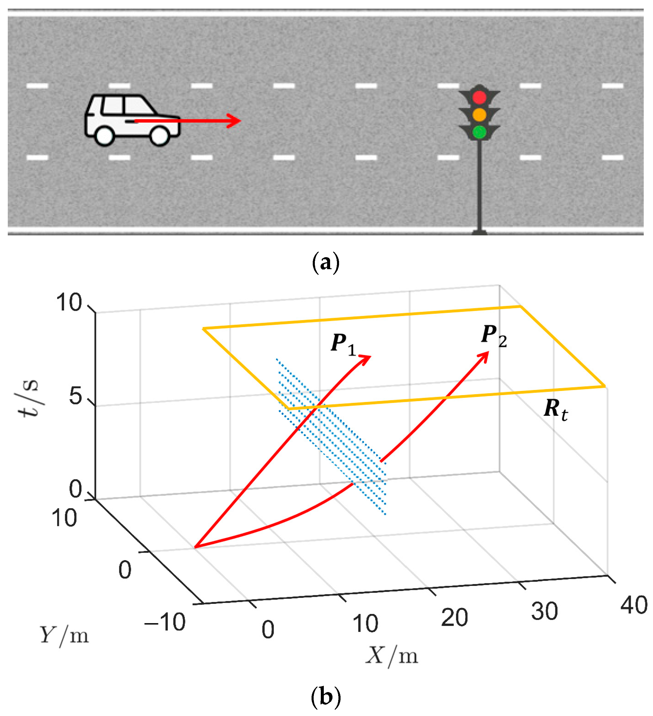
Traffic light scenarios are common scenarios on urban roads. An example traffic light scenario is shown in Figure 15, where the light will turn red after the third second and then turn green after the eighth second. For our spatial–time model, no complex logic is required to obtain the pass options. In P 1 the vehicle deaccelerates and waits for the light turns to green. In P 2 the vehicle accelerates and passes before the light turns red.

5. Trajectory Planning Compatibility

The spatial–time environment model is compatible with existing planning approaches. To demonstrate the benefits of the proposed cognitive spatial–time environment model for trajectory planning, a simple hybrid A* planning approach [29] is applied. In fact, it is a modified simple hybrid A star planner, with an additional speed search strategy mentioned in Chapter A, Section 3. The HFSM approach from the literature [15] is selected as the control group.

5.1. Scenario 1

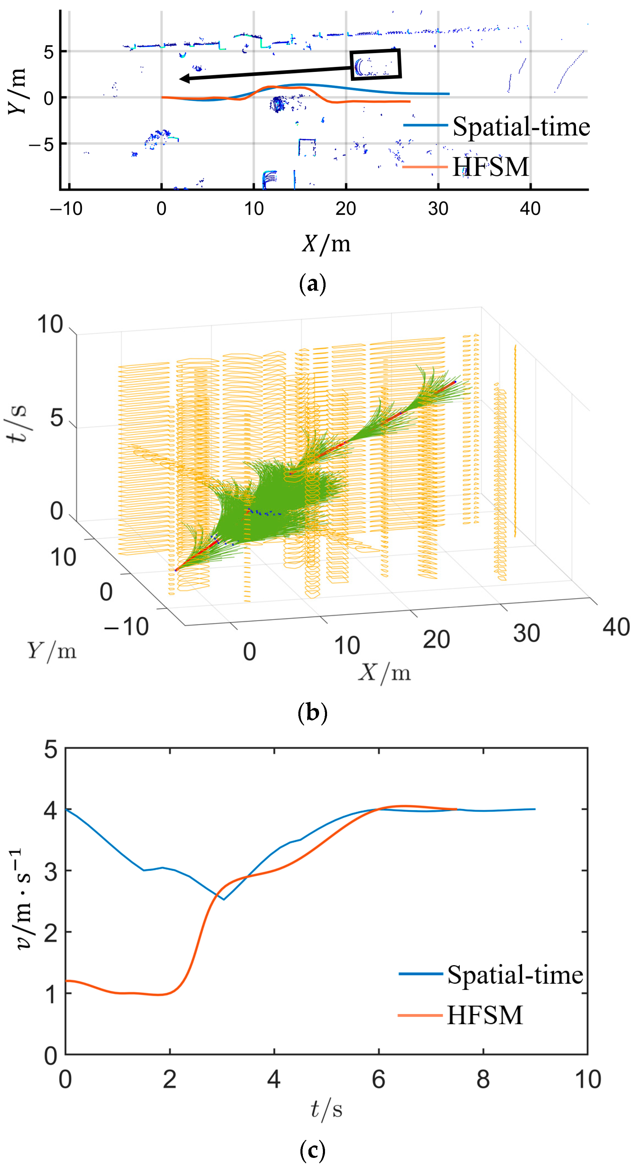
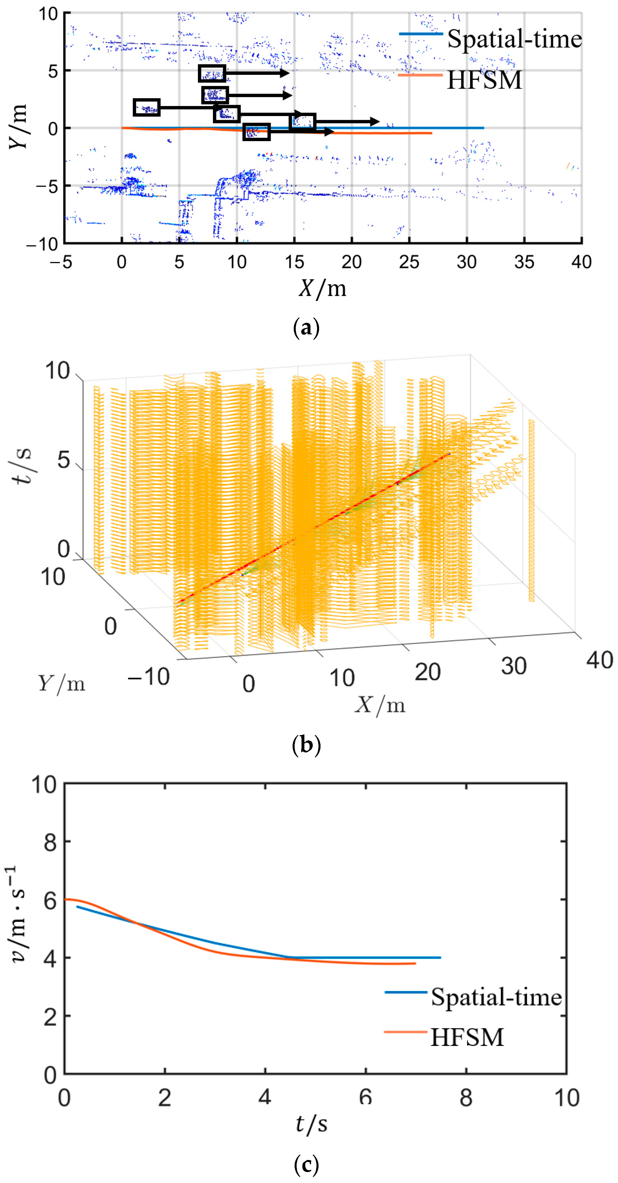
Figure 16 shows the trajectory planning results of a dynamic obstacle avoidance scenario with one dynamic obstacle and multiple static obstacles. This case is deployed to reflect the capability of the proposal to evade the dynamic obstacle. The black frame represents a moving vehicle approaching in the opposite direction, and the blue dots represent static obstacles. The ego vehicle needs to drive forward. To that end, the trajectory planner needs to balance efficiency and safety, obtaining a feasible path and speed of the ego vehicle to avoid collisions. The initial speed of the vehicle is 4 m/s; there is a static obstacle at an offset of 0.6 m in front of the vehicle and a dynamic obstacle traveling 4.3 m/s in the opposite direction in front and to the left. The planning result is represented by the brown line (projection in the X–Y domain of the planned trajectory). Figure 16b shows what the spatial–time environment model looks like in this scenario. The yellow boxes represent obstacles, the trajectory search process is represented by the green line, and the final trajectory is represented by the brown line. The speed profile of the planned trajectory is shown in Figure 16c. Obviously, the brown line bypasses all obstacles, providing a trajectory for the ego vehicle. The trajectory planned by the spatial–time approach guides the vehicle from 4 m/s to 2.8 m/s at 2.5 s to avoid the dynamic obstacle coming from the opposite direction. Then, the vehicle accelerates and veers to the left to overtake the static obstacle, after the dynamic obstacle has been identified as no threat. The HFSM approach also presents a trajectory of slowing down to avoid the dynamic obstacle before avoiding the static obstacle ahead. However, the passage is less efficient than the spatial–time approach, as the speed varies more.

5.2. Scenario 2

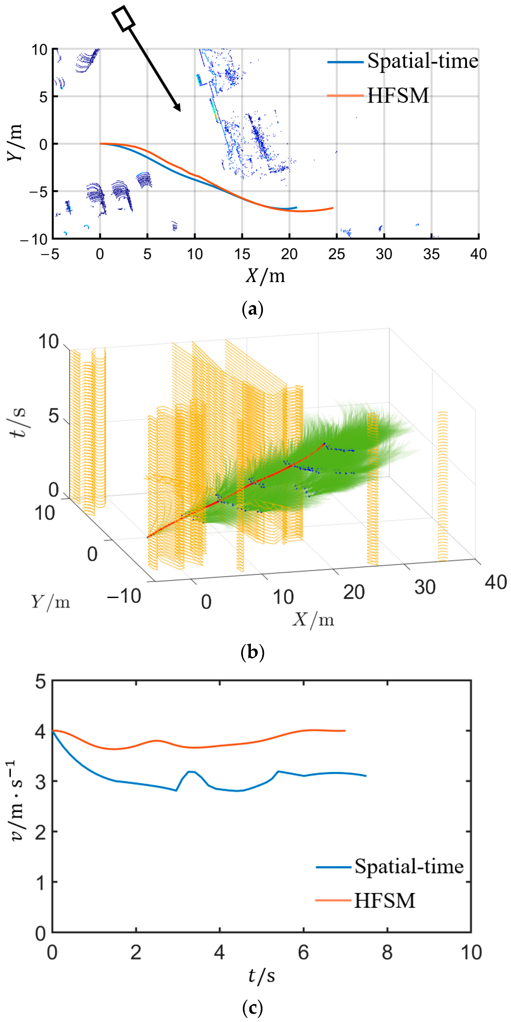
Figure 17 shows the trajectory planning results of a right turn scenario with a dynamic obstacle cut-in, which allows the approach to be tested for its dynamic avoidance and planning capabilities in half-structured road scenarios. The ego vehicle runs at an initial speed of 4 m/s, and there is a dynamic cut-in vehicle at a constant speed of 3.5 m/s. The planning result is shown in Figure 17a, the planning process using a spatial–time approach is shown Figure 17b, and the speed profile is shown in Figure 17c. The trajectory planned by the spatial–time approach guides the vehicle past the junction after a slight deceleration from 4 m/s to 3 m/s. The HFSM approach guides the vehicle past the junction at a speed of around 4 m/s. In both approaches, the dynamic obstacle is judged to pose no hazard to the vehicle. The trajectories of the vehicle exhibit only a slight additional offset to the right to avoid the incoming dynamic obstacle.

5.3. Scenario 3

Figure 18 shows the trajectory planning results of a vehicle follow scenario. The adaptability of the approach to vehicle following scenarios can be tested. The ego vehicle runs at an initial speed of 6 m/s, and there are dynamic obstacles moving at a constant speed of 4 m/s. The planning result is shown in Figure 18a, the planning process using a spatial–time approach is shown Figure 18b, and the speed profile is shown in Figure 18c. The planned trajectories exhibit the “vehicle follow” driving behavior, in which scenario the ego vehicle follows the vehicle in front of it after slowing down to 4 m/s. The spatial–time approach has a smoother trajectory and less lateral fluctuations then the HFSM approach.

5.4. Scenario 4

Figure 19 shows the trajectory planning results of a cut-in scenario, which can test the dynamic hazard assessment and dynamic obstacle avoidance capabilities. The ego vehicle runs at an initial speed of 12 m/s, and there are two vehicle cut-ins to the trajectory of ego vehicle. The planning result is shown in Figure 19a, the planning process using a spatial–time approach is shown Figure 19b, and the speed profile is shown in Figure 19c. Both the spatial–time approach and the HFSM approach identify that the two dynamic obstacles cutting ahead pose a hazard to the ego vehicle, and then guide the vehicle to the left to avoid the two dynamic obstacles. The spatial–time approach has a smoother trajectory, showing a sequence of driving behaviors of changing lanes to the left, driving along the lane and changing lanes to the right. The HFSM approach shows the same driving behavior as the spatial–time approach, but the trajectory is less flexible as the planning process is more regular and rule-based than the spatial–time approach.

5.5. Scenario 5

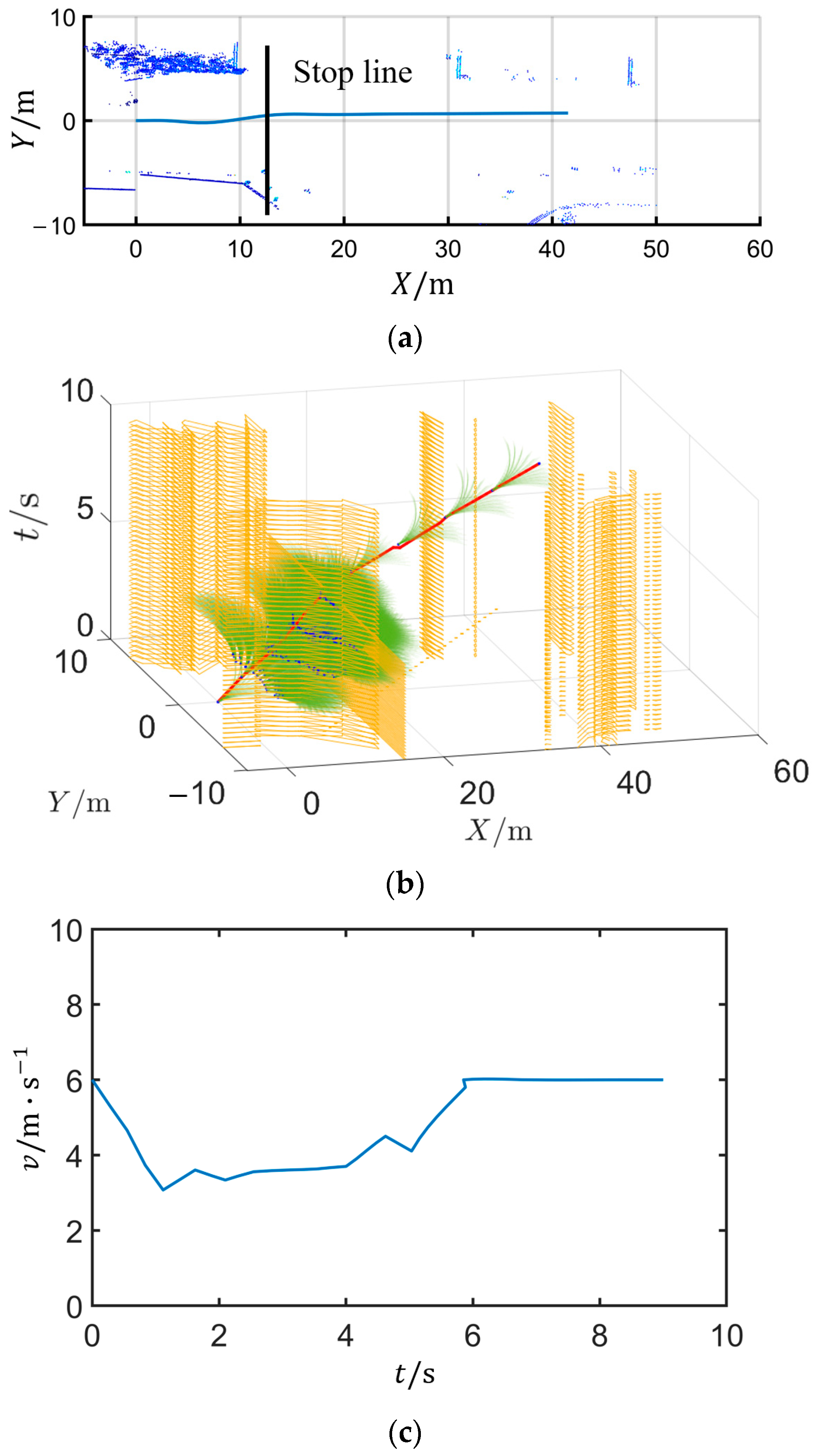
Figure 20 shows the trajectory planning results of a traffic light control scenario. The initial speed of the vehicle is 6 m/s and the stop line is 12 m ahead of the vehicle. The movement of the vehicle passing through the junction is controlled by a traffic signal which is red (no passing) from the 0 s moment to the 4 s moment. The signal then switches to green (passing allowed). This scenario is a typical traffic-signal-controlled junction scenario. The planning result is shown in Figure 20a, the planning process using a spatial–time approach is shown Figure 20b, and the speed profile is shown in Figure 20c. The trajectory planned by the spatial–time approach guides the vehicle from an initial speed of 6 m/s to a gradual deceleration to 4 m/s at the 1 s moment, and maintains a speed of 4 m/s until the 5th second. Then, the vehicle accelerates to 6 m/s. The process is similar to the behavior of a human driver who chooses to slow down slightly and wait for the signal to change, rather than stopping at the stop line and waiting for the signal to change.

6. Conclusions

This paper introduced a cognitive spatial–time environment model for autonomous vehicles. The underlying highlights are summarized as follows: (1) A spatial–time environment model was defined and established, where common features between scenarios were analyzed, and static and dynamic objects were converted into spatial–time occupancy and projected into the model. (2) The trajectory planning problem in multiple scenarios was analyzed, as well as the scenario adaptation of the spatial–time environment model. It was shown that the spatial–time environment model can be adapted to multiple scenarios, providing the possibility of multi-scenario adaptation of trajectory planning approaches. (3) The integrated trajectory planning capabilities using the spatial–time environment model were evaluated using a hybrid A* algorithm. The simulation results showed that the proposal could solve planning problems in multiple scenarios without changes in the planning algorithm, obtain integrated trajectories in the path and speed domains, and bring higher scenario adaptability to trajectory planning for autonomous vehicles.
Our future work will comprise the following goals: (1) Novel planning approaches will be applied to the cognitive spatial–time environment model to explore trajectory planning performances in complex dynamic corner case scenarios. SOTIF (Safety of the Intended Functionality)-related issues and more road scenarios from around the world will be introduced. (2) The combination of artificial potential fields and the spatial–time environment model will be studied to solve the local minimum problem, which is the problem of not being able to obtain feasible trajectories in some scenarios.

Author Contributions

Conceptualization, R.C., J.H. and M.Z.; methodology, R.C. and L.Z.; software, R.C., X.Z. and M.Z.; resources, J.H.; data curation, L.Z.; writing R.C.; funding acquisition R.C. and J.H. All authors have read and agreed to the published version of the manuscript.

Funding

All the authors would like to express our gratitude to all those who helped us improve this work. The authors are grateful for the support provided by “Hubei Provincial Department of Science and Technology (2020AAA001)”, “Hubei Provincial Department of Science and Technology (2022AAA001)”, and “The Fundamental Research Funds for the Central Universities (2020-YB-020)”.

Institutional Review Board Statement

Not applicable.

Informed Consent Statement

Not applicable.

Data Availability Statement

The data used to support the findings of this study are available from the corresponding author upon request.

Acknowledgments

The authors wish to thank Kai Cao from Dongfeng Usharing Technology Co., Ltd., for valuable discussion and the constructive comments on the experiments.

Conflicts of Interest

The authors declare that they have no known competing financial interest or personal relationships that could have appeared to influence the work reported in this paper.

References

  1. Gonzalez, D.; Perez, J.; Milanes, V.; Nashashibi, F. A Review of Motion Planning Techniques for Automated Vehicles. IEEE Trans. Intell. Transp. Syst. 2016, 17, 1135–1145. [Google Scholar] [CrossRef]
  2. Yurtsever, E.; Lambert, J.; Carballo, A.; Takeda, K. A Survey of Autonomous Driving: Common Practices and Emerging Technologies. IEEE Access 2020, 8, 58443–58469. [Google Scholar] [CrossRef]
  3. Chu, Y.; Wu, Z.; Yue, Y.; Zhu, X.; Lim, E.G.; Paoletti, P. PK-APF: Path-Keeping Algorithm for USVs Based on Artificial Potential Field. Appl. Sci. 2022, 12, 8201. [Google Scholar] [CrossRef]
  4. Li, B.; Zhang, Y.; Shao, Z.; Jia, N. Simultaneous versus Joint Computing: A Case Study of Multi-Vehicle Parking Motion Planning. J. Comput. Sci. 2017, 20, 30–40. [Google Scholar] [CrossRef]
  5. Kim, D.J.; Lee, S.-H.; Chung, C.C. Object Vehicle Motion Prediction Based on Dynamic Occupancy Grid Map Utilizing Cascaded Support Vector Machine. In Proceedings of the 2019 19th International Conference on Control, Automation and Systems (ICCAS), Jeju, Korea, 15–18 October 2019; Volume 2019-Octob, pp. 496–500. [Google Scholar]
  6. Wang, J.; Wu, J.; Zheng, X.; Ni, D.; Li, K. Driving Safety Field Theory Modeling and Its Application in Pre-Collision Warning System. Transp. Res. Part C Emerg. Technol. 2016, 72, 306–324. [Google Scholar] [CrossRef]
  7. Jurecki, R.S.; Stańczyk, T.L. Modeling Driver’s Behaviour While Avoiding Obstacles. Appl. Sci. 2023, 13, 616. [Google Scholar] [CrossRef]
  8. Wahab, M.N.A.; Nefti-Meziani, S.; Atyabi, A. A Comparative Review On Mobile Robot Path Planning: Classical or Meta-Heuristic Methods? Annu. Rev. Control 2020, 50, 233–252. [Google Scholar] [CrossRef]
  9. Xin, Y.; Liang, H.; Mei, T.; Huang, R.; Du, M.; Sun, C.; Wang, Z.; Jiang, R. A New Occupancy Grid of the Dynamic Environment for Autonomous Vehicles. In Proceedings of the 2014 IEEE Intelligent Vehicles Symposium Proceedings, Dearborn, MI, USA, 8–11 June 2014; pp. 787–792. [Google Scholar]
  10. Sedighi, S.; Nguyen, D.-V.; Kapsalas, P.; Kuhnert, K.-D. Implementing Voronoi-Based Guided Hybrid A* in Global Path Planning for Autonomous Vehicles. In Proceedings of the 2019 IEEE Intelligent Transportation Systems Conference (ITSC), Auckland, New Zealand, 27–30 October 2019; pp. 3845–3852. [Google Scholar]
  11. Ammar, A.; Bennaceur, H.; Châari, I.; Koubâa, A.; Alajlan, M. Relaxed Dijkstra and A* with Linear Complexity for Robot Path Planning Problems in Large-Scale Grid Environments. Soft Comput. 2016, 20, 4149–4171. [Google Scholar] [CrossRef]
  12. Li, B.; Ouyang, Y.; Li, L.; Zhang, Y. Autonomous Driving on Curvy Roads Without Reliance on Frenet Frame: A Cartesian-Based Trajectory Planning Method. IEEE Trans. Intell. Transp. Syst. 2022, 23, 15729–15741. [Google Scholar] [CrossRef]
  13. Hamid, U.Z.A.; Ariff, M.H.M.; Zamzuri, H.; Saito, Y.; Zakaria, M.A.; Rahman, M.A.A.; Raksincharoensak, P. Piecewise Trajectory Replanner for Highway Collision Avoidance Systems with Safe-Distance Based Threat Assessment Strategy and Nonlinear Model Predictive Control. J. Intell. Robot. Syst. 2018, 90, 363–385. [Google Scholar] [CrossRef]
  14. Jiang, Y.; Jin, X.; Xiong, Y.; Liu, Z. A Dynamic Motion Planning Framework for Autonomous Driving in Urban Environments. In Proceedings of the 2020 39th Chinese Control Conference (CCC), Shenyang, China, 27–29 July 2020; Volume 2020-July, pp. 5429–5435. [Google Scholar]
  15. Hu, J.; Chen, R.; Xu, W.; Lu, R. An Event-Triggered Real-Time Motion Planning Strategy for Autonomous Vehicles. Proc. Inst. Mech. Eng. Part C J. Mech. Eng. Sci. 2022, 236, 10332–10348. [Google Scholar] [CrossRef]
  16. Hafeez, F.; Ullah Sheikh, U.; Mas’ud, A.A.; Al-Shammari, S.; Hamid, M.; Azhar, A. Application of the Theory of Planned Behavior in Autonomous Vehicle-Pedestrian Interaction. Appl. Sci. 2022, 12, 2574. [Google Scholar] [CrossRef]
  17. Zou, S.; Luan, Z.; Zhao, W.; Wang, C. Personalized Design Strategy of Vehicle Steer-by-Wire Characteristics Considering Driving Style. Proc. Inst. Mech. Eng. Part C J. Mech. Eng. Sci. 2023, 237, 253–266. [Google Scholar] [CrossRef]
  18. Bergman, K.; Ljungqvist, O.; Axehill, D. Improved Path Planning by Tightly Combining Lattice-Based Path Planning and Optimal Control. IEEE Trans. Intell. Veh. 2021, 6, 57–66. [Google Scholar] [CrossRef]
  19. Li, B.; Kong, Q.; Zhang, Y.; Shao, Z.; Wang, Y.; Peng, X.; Yan, D. On-Road Trajectory Planning with Spatio-Temporal RRT* and Always-Feasible Quadratic Program. In Proceedings of the 2020 IEEE 16th International Conference on Automation Science and Engineering (CASE), Hong Kong, China, 20–21 August 2020; Volume 2020-Augus, pp. 942–947. [Google Scholar]
  20. Zong, C.; Han, X.; Zhang, D.; Liu, Y.; Zhao, W.; Sun, M. Research on Local Path Planning Based on Improved RRT Algorithm. Proc. Inst. Mech. Eng. Part D J. Automob. Eng. 2021, 235, 2086–2100. [Google Scholar] [CrossRef]
  21. Luo, J.; Li, S.; Li, H.; Xia, F. Intelligent Network Vehicle Driving Risk Field Modeling and Path Planning for Autonomous Obstacle Avoidance. Proc. Inst. Mech. Eng. Part C J. Mech. Eng. Sci. 2022, 236, 8621–8634. [Google Scholar] [CrossRef]
  22. Fan, H.; Zhu, F.; Liu, C.; Zhang, L.; Zhuang, L.; Li, D.; Zhu, W.; Hu, J.; Li, H.; Kong, Q. Baidu Apollo EM Motion Planner. arXiv 2018, arXiv:1807.08048. [Google Scholar]
  23. Hidalgo, C.; Lattarulo, R.; Perez, J.; Asua, E. Hybrid Trajectory Planning Approach for Roundabout Merging Scenarios. In Proceedings of the 2019 IEEE International Conference on Connected Vehicles and Expo (ICCVE), Graz, Austria, 4–8 November 2019; pp. 1–6. [Google Scholar]
  24. García Cuenca, L.; Puertas, E.; Fernandez Andrés, J.; Aliane, N. Autonomous Driving in Roundabout Maneuvers Using Reinforcement Learning with Q-Learning. Electronics 2019, 8, 1536. [Google Scholar] [CrossRef] [Green Version]
  25. Zhu, H.; Han, T.; Alhajyaseen, W.K.M.; Iryo-Asano, M.; Nakamura, H. Can Automated Driving Prevent Crashes with Distracted Pedestrians? An Exploration of Motion Planning at Unsignalized Mid-Block Crosswalks. Accid. Anal. Prev. 2022, 173, 106711. [Google Scholar] [CrossRef]
  26. Rahmati, Y.; Talebpour, A. Towards a Collaborative Connected, Automated Driving Environment: A Game Theory Based Decision Framework for Unprotected Left Turn Maneuvers. IEEE Intell. Veh. Symp. Proc. 2017, 1316–1321. [Google Scholar] [CrossRef]
  27. Mazare, M.; Asharioun, H.; Davoudi, E.; Mokhtari, M. Distributed Finite-Time Neural Network Observer-Based Consensus Tracking Control of Heterogeneous Underwater Vehicles. Ocean Eng. 2023, 272, 113882. [Google Scholar] [CrossRef]
  28. Chen, R.; Hu, J.; Xu, W. An RRT-Dijkstra-Based Path Planning Strategy for Autonomous Vehicles. Appl. Sci. 2022, 12, 11982. [Google Scholar] [CrossRef]
  29. Sheng, W.; Li, B.; Zhong, X. Autonomous Parking Trajectory Planning with Tiny Passages: A Combination of Multistage Hybrid A-Star Algorithm and Numerical Optimal Control. IEEE Access 2021, 9, 102801–102810. [Google Scholar] [CrossRef]
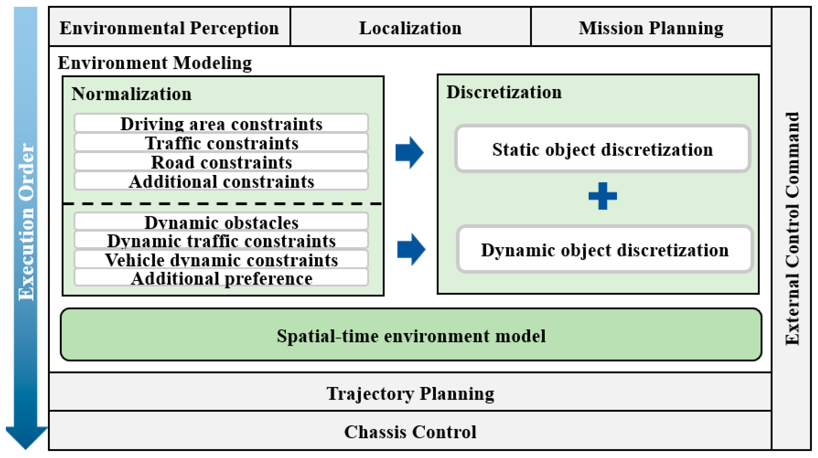
Figure 1. Strategy architecture.
Applsci 13 03984 g001
Figure 2. Spatial–time environment model.
Applsci 13 03984 g002
Figure 3. Example M s t with dynamic objects. (a) Speed calculation approach; (b) Speed profile.
Applsci 13 03984 g003
Figure 4. Example M s t with static objects.
Applsci 13 03984 g004
Figure 5. Example M s t with static objects.
Applsci 13 03984 g005
Figure 6. Example M s t with static objects.
Applsci 13 03984 g006
Figure 7. Example scenario with collision checking.
Applsci 13 03984 g007
Figure 8. Road cost map at time t .
Applsci 13 03984 g008
Figure 9. Static obstacle avoidance scenario. (a) Scenario diagram; (b) Spatial–time model of the scenario.
Applsci 13 03984 g009aApplsci 13 03984 g009b
Figure 10. Dynamic overtaking scenario. (a) Scenario diagram; (b) Spatial–time model of the scenario.
Applsci 13 03984 g010
Figure 11. Dynamic Cut-in Scenario. (a) Scenario diagram; (b) Spatial–time model of the scenario.
Applsci 13 03984 g011
Figure 12. Lane merging scenario. (a) Scenario diagram; (b) Spatial–time model of the scenario.
Applsci 13 03984 g012
Figure 13. Unprotected left turns with traffic. (a) Scenario diagram; (b) Spatial–time model of the scenario.
Applsci 13 03984 g013aApplsci 13 03984 g013b
Figure 14. Roundabout entry and exit scenario. (a) Scenario diagram; (b) Spatial–time model of the scenario.
Applsci 13 03984 g014
Figure 15. Traffic light scenario. (a) Scenario diagram; (b) Spatial–time model of the scenario.
Applsci 13 03984 g015
Figure 16. Scenario 1. (a) Environmental point cloud and planned path; (b) Spatial–time environment model with hybrid A* planned trajectory; (c) Speed profile.
Applsci 13 03984 g016
Figure 17. Scenario 2. (a) Environmental point cloud and planned path; (b) Spatial–time environment model with hybrid A* planned trajectory; (c) Speed profile.
Applsci 13 03984 g017
Figure 18. Scenario 3. (a) Environmental point cloud and planned path; (b) Spatial–time environment model with hybrid A* planned trajectory; (c) Speed profile.
Applsci 13 03984 g018
Figure 19. Scenario 4. (a) Environmental point cloud and planned path; (b) Spatial–time environment model with hybrid A* planned trajectory; (c) Speed profile.
Applsci 13 03984 g019
Figure 20. Scenario 5. (a) Environmental point cloud and planned path; (b) Spatial–time environment model with hybrid A* planned trajectory; (c) Speed profile.
Applsci 13 03984 g020
Disclaimer/Publisher’s Note: The statements, opinions and data contained in all publications are solely those of the individual author(s) and contributor(s) and not of MDPI and/or the editor(s). MDPI and/or the editor(s) disclaim responsibility for any injury to people or property resulting from any ideas, methods, instructions or products referred to in the content.