Open-Set Specific Emitter Identification Based on Prototypical Networks and Extreme Value Theory

Abstract

Much research has focused on classification within a closed set of emitters, while emitters outside this closed set are misclassified. This paper proposes an open-set recognition model based on prototypical networks and extreme value theory to solve the problem of specific emitter identification in open-set scenes and further improve the recognition accuracy and robustness. Firstly, a one-dimensional convolutional neural network was designed for recognizing I/Q signals, and a squeeze-and-excitation block with an attention mechanism was added to the network to increase the weights of the feature channels with high efficiency. Meanwhile, the recognition was improved by group convolution and channel shuffle. Then, the network was trained with the joint loss function based on prototype learning to complete the separation of intra-class signals and the aggregation of inter-class signals in the feature space. After the training, the Weibull model was fitted for pre-defined classes by incorporating the extreme value theory. Finally, the classification results were obtained according to the known classes and the Weibull model, effectively completing the open-set recognition. The simulation results showed that the proposed model had a higher recognition performance and robustness compared with other classical models for signals collected from five ZigBee and ten USRP 310 devices.

1. Introduction

The large-scale application of wireless communication technology and the advent of the Internet of Things era have prompted the rapid development of a large number of communication devices, along with serious challenges in the fields of communication security and signal reconnaissance. Traditional MAC address and secret key authentication methods are easy to forge and crack, and relying on signal analysis methods to track and identify signals can no longer meet the needs of reconnaissance in complex electromagnetic environments. Specific emitter identification (SEI) can accomplish the authentication and identification of individual emitters by extracting the inherent fingerprint features in signals of different emitters due to hardware manufacturing and other effects [1]. In the field of electronic reconnaissance, the identification of individual features can effectively provide information on non-cooperative targets, track the spatial location of signals, analyze the electromagnetic situation on battlefields, and generate valuable intelligence. In addition, SEI combined with traditional authentication methods, such as secret key and MAC address, can strengthen the recognition and identity authentication of illegal wireless communication devices [1,2] and improve the security performance of communication systems.

According to the working state of the communication emitters, the signal fingerprint features can be divided into transient features and steady-state features. The differences in transient features are obvious and easy to distinguish, but the extraction of transient features requires high-precision equipment and acquisition conditions, since it is susceptible to noise [3,4,5,6]. In view of the difficulty of detecting the transient starting point of the signal, Ref. [7] several methods for detecting transient starting points have been developed. Among them, the energy criterion method based on the instantaneous amplitude characteristics was recently shown to be superior.

Compared with transient features, steady-state features are easy to obtain; therefore, the method of extracting RF fingerprints based on steady-state features has been widely researched and applied. For example, the high-order cumulant detection function was constructed to extract the boot signal envelope, and the envelope fractal feature was used to cluster the signal extraction results, which could identify the fingerprinting characteristics of FH radio stations [8]. The fractal features of the FH signal extracted by this method could effectively suppress the noise impact. Ref. [9] proposed square integral bispectra (SIB) to extract the unique stray features of an individual transmitted signal, and the principal component analysis (PCA) method was utilized to extract a low-dimensional classification vector. Then, a support vector machine (SVM) based on the Gaussian kernel function was implemented to complete the classification. The proposed model was highly accurate and robust even in the presence of excessive noise. Ref. [10] proposed an emitter identification based on variational mode decomposition and spectral features (VMD-SF). This method had a lower computational cost than the VMD-EM² method and the existing EMD-EM² method. However, these feature extraction and classification methods have high complexity. The extracted features are not comprehensive enough, the generalization is not strong, and the recognition accuracy is generally low.

With the rapid development of deep learning technology [11], many researchers have applied it to SEI or signal recognition. For example, Ref. [12] applied the Hilbert–Huang transform to the received signal and converted the Hilbert spectrum into a grayscale image. Then, residual networks were used to learn the visual differences reflected in the Hilbert spectrum images. The simulation results validated that the Hilbert spectrum image was a successful signal representation and demonstrated that the fingerprints extracted from raw images using deep learning were more effective and robust than the expert ones. Similarly, the differential constellation trace figure (DCTF) [13], bispectrum [14] and nonlinear features of the power amplifier, and modulator distortion features [15] of the signal are recognized by different convolutional neural networks (CNNs) for SEI, and all of these methods present substantial performance improvements over traditional methods. However, converting signals into two-dimensional forms such as images increases the model complexity and may cause the loss of some original information related to the signals. Therefore, many researchers have used neural networks to recognize the original sequence signals directly; for example, using one-dimensional CNNs to accomplish the feature extraction and classification of I/Q sequence signals [16,17,18]. Further, recognition methods based on hybrid networks and complex neural networks have also been proposed [19,20], such as the fusion of CNNs and LSTM. In [19], deep bidirectional long short-term memory (DBi-LSTM) and a one-dimensional residual convolution network with dilated convolution and a squeeze-and-excitation block (Conv-OrdsNet) were devised to extract temporal structure features directly from baseband I/Q samples. Moreover, a data augmentation method was used to overcome the interference of unreliable features. The proposed model could effectively extract reliable RF fingerprinting features from I/Q samples, and the classification results were better than those of most existing methods. Meanwhile, ensemble neural networks were proposed for the recognition of the fusion features of graphs and the sequence features of signals [21]. These methods made use of powerful feature extraction techniques, the self-learning of deep learning, and corresponding data processing methods, which greatly improved their classification performance. In addition, a multi-channel model was established to reduce the effect of channel changes on individual recognition, which effectively improved the recognition accuracy and robustness of the models under the conditions of channel changes and noise [22]. Based on the communication of the physical layer and the support vector data description (SVDD) algorithm, Ref. [23] established a radio frequency fingerprint authentication model for communication devices. Ref. [24] proposed a light-weight radio frequency fingerprinting identification (RFFID) scheme combined with a two-layer model to realize authentication for a large number of resource-constrained terminals under a mobile edge computing (MEC) scenario. The results showed that the novel method could achieve a higher recognition rate than that of the traditional RFFID method by using the wavelet feature effectively, which demonstrated the efficiency of the proposed method. Ref. [25] defined a device-specific unique fingerprint by analyzing solely the inter-arrival time of packets as a feature to identify a device. Thus, they obtained a superior identification model compared with ResNet 50-layer and basic CNN 5-layer architectures.

Most previous research on SEI was based on closed-set scenes, i.e., the same classes of samples were used for both validation and training. However, recognition algorithms for closed-set scenes are difficult to apply to actual electromagnetic environments with open-set properties. In open-set scenes, the samples to be tested may contain new classes that do not appear in the training set, and models trained in a closed set will recognize the new samples as known classes, thus seriously affecting the recognition accuracy. Several researchers have started to research SEI in open-set scenes. Refs. [26,27] used OpenMax [28] based on the extreme value theory (EVT) to recognize the communication emitters and high-resolution range profiles of radar, achieving performance advantages compared with the traditional open-set recognition model. In order to enhance the discriminative power of deeply learned features, Ref. [29] proposed center loss for face recognition tasks. The center loss simultaneously learned a center for deep features of each class and penalized the distances between the deep features and their corresponding class centers. It significantly improved upon previous results and is expected to be used for open-set recognition. Ref. [30] proposed an unsupervised class-distance learning method, which used an auxiliary dataset containing only open classes to learn the decision boundary between closed and open sets and achieved improved results.

In recent years, prototypical networks combining prototype learning ideas and deep neural networks have been used for image recognition under few-shot conditions [31], class-incremental learning [32], and open-set recognition [33]. These methods have achieved better recognition performance compared with traditional CNNs. Prototypical networks have obvious advantages in solving few-shot problems and improving generalization performance. Additionally, the classification principle of prototypical networks is more favorable for open-set recognition.

Based on this, we propose an open-set SEI model for one-dimensional sequence signals by combining prototypical networks and EVT. We creatively introduced an attention mechanism and ShuffleNet into a one-dimensional neural network and combined this prototype network and extreme value theory for the first time to obtain a higher recognition performance and robustness. The results of the experiments on the dataset collected by 5 ZigBee devices and 10 USRP 310 devices showed that the proposed model had a higher recognition accuracy than other models such as OpenMax. The recognition accuracy of the five ZigBee devices reached 95% at 0 dB, and it reached over 90% at a mixed SNR of −4–10 dB for the 10 USRP 310 devices. The contributions of the proposed model are as follows:

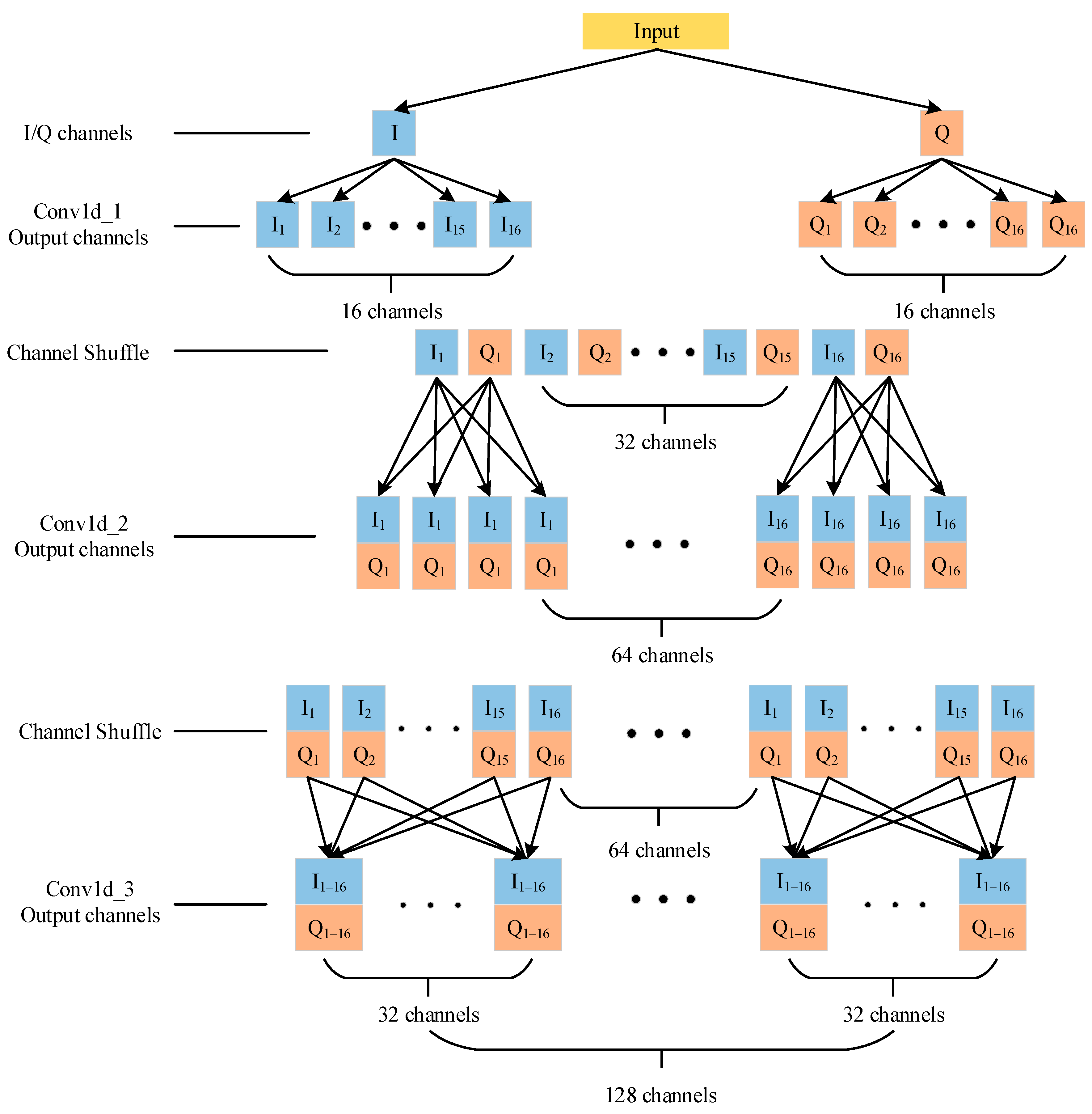
• A one-dimensional CNN integrating an attention mechanism was designed. Meanwhile, group convolution and channel shuffle were introduced into the network, which reduced the complexity and overfitting and effectively improved the recognition performance.
• Prototype learning was combined with the one-dimensional CNN. Distance-based cross-entropy loss and prototype loss were used to train the network to complete the separation of inter-class signals and the aggregation of intra-class signals in the feature space.
• Combining EVT, Weibull models were fitted for each known class based on the distance from the sample features to the mean features. The open-set recognition was completed based on the Weibull models and the distance between the features of the test samples and the mean features of known classes.

The rest of the paper is organized as follows. Section 2 introduces the classification principle of the prototypical networks and the basic theory for applying EVT to open-set recognition. Section 3 presents the design of the open-set recognition model, including the network structure, classification algorithm, and loss function. Simulation experiments on five ZigBee devices and an analysis of the simulation results are provided in Section 4. Finally, a brief conclusion is presented in Section 5.

2. Prototypical Networks and Extreme Value Theory

2.1. Prototypical Networks

Prototypical networks, combining neural networks and prototype learning, use the distance between the sample features and the prototypes to measure the attribution of samples, leading to a wide range of applications in fields such as few-shot learning [26]. Prototype learning is a classical algorithm in pattern recognition [34]. With the development of neural networks, prototype learning methods have been integrated into the CNN framework for better performance. Previous CNN models used SoftMax to normalize the output of the fully connected layer and classify the input sample $x$ with the highest probability. The classification is based on:

$$\left\{\begin{array}{l}x\in class\arg \underset{y=1}{\overset{N}{\max }}p(y|x)\\ p(y|x)=\frac{\exp ({\xi }_y)}{{\displaystyle \sum _{i=1}^N\exp ({\xi }_i)}}\end{array}\right.$$

(1)

where $p(y|x)$ represents the probability that sample $x$ belongs to the class $y$; ${\xi }_i$ represents the network output of class $i$, where $i\in \left\{1,2,\cdots ,N\right\}$; and N represents the number of known classes. When using prototypical networks for classification, the networks can learn a prototype $a_i$ for each class. Then, the samples can be classified into the class with the closest prototype. The process can be expressed as:

$$x\in class \arg \underset{i=1}{\overset{N}{\max }}{g}_i(x)$$

(2)

where $g_i(x)$ is the classification function of class $i$ [33]. It can also be expressed as:

$$g_i(x)=-{‖f(x;\theta )-a_i‖}_2^2$$

(3)

where $f(x;\theta )$ represents the neural network feature extractor, and $\theta$ represents the network parameters. $f(x;\theta )$ and the prototype $a_i$ can be learned jointly [33]. During the learning process, the prototype of a certain class is continuously pushed towards the sample features of that class, while the prototypes of other classes are kept away from the sample features of that class.

Prototype learning transforms the classification into the nearest neighbor problem in the feature vector space. The addition of the feature extraction advantages of neural networks can effectively improve the generalization performance and alleviate overfitting. We can also see that the classification principle of prototypical networks and the metrics method based on distance are more conducive to recognizing unknow classes.

2.2. Extreme Value Theory

EVT is a theory dealing with the maximum and minimum values of a probability distribution and is mainly used to predict the probability of extreme events. In 1928, R.A. Fisher and L.H.C. Tipper published their famous paper on EVT [35], which showed that low-probability events obeyed another probability distribution. By analyzing the occurrence of past extreme events and finding their distribution patterns, it is possible to calculate the probability that an extreme event may occur in the future, including the possibility of new events. For example, using historical data of the lowest temperature in a particular location, it is possible to predict the future lowest temperature, including the probability of the record lowest temperatures occurring.

EVT is related to many widely used distributions such as the Weibull distribution. The authors of [36] indicated that within multiple independent distributions, the set of extreme values necessarily converges to an extreme value distribution. Usually, the extreme values in a set of data can be represented by the Weibull distribution. The probability density of the Weibull distribution is expressed as:

$$f_1(x;\alpha ,\beta )=\left\{\begin{array}{ll}\frac{\beta }{\alpha }{\left(\frac{x}{\alpha }\right)}^{\beta -1}{e}^{-{\left(\frac{x}{\alpha }\right)}^{\beta }}& x\ge 0\\ 0& x<0\end{array}\right.$$

(4)

where $x$ is the random variable, $\alpha >0$ is the scale parameter, and $\beta >0$ is the shape parameter. The cumulative distribution function of the Weibull distribution is expressed as:

$$f_2(x;\alpha ,\beta )=\left\{\begin{array}{ll}1-e^{-{\left(\frac{x}{\alpha }\right)}^{\beta }}& x\ge 0\\ 0& x<0\end{array}\right.$$

(5)

According to the properties of the Weibull cumulative distribution function, the Weibull model can be fitted using several maximum values of each class. When the input is far from the distribution of a class, it is probably judged as an extreme value or an outlier by the Weibull model. Thus, the network output of the test samples can be weighted according to the probability, and the score of the samples belonging to the unknown classes can be obtained, which effectively enhances the robustness of open-set recognition.

3. Recognition Model

3.1. Model Framework

The proposed open-set SEI model uses the prototypical networks as the basic structure and incorporates EVT to achieve open-set recognition for I/Q sequence data. The model framework is shown in Figure 1 and is divided into three main modules.

The data-processing module preprocesses the data and then forms the training set and test set according to the preset ratio. In the following training process, classification is performed by the distance from the sample features to the prototypes, and a tight feature space is learned for each class using the joint loss function. After the training, the Weibull model is fitted for each class separately. Thirdly, the testing module obtains the network output of the test samples. Then, the distance of the test samples to the mean features of all known classes is calculated, and the Weibull cumulative distribution probability of the test samples is obtained based on this distance. Finally, the network output is revised by this probability, and the scores of the test samples belonging to the known and unknown classes are obtained.

3.2. Network Structure

The structure of the open-set recognition network is shown in Figure 2. In this study, we directly processed the sequence data with low complexity, so the designed network structure was based on a relatively simple one-dimensional CNN. Four convolution layers exist in the network, and the number of convolutional kernels in each layer is 32, 64, 128, and 256, respectively. A maximum pooling layer with a kernel of two was added after each convolutional layer to reduce the complexity and overfitting of the model, and the final output dimension was reduced by the four-layer network to fully extract the deep features of the data.

The convolution kernel size of each convolution layer is $1\times 9$. Using larger convolutional kernels allows one to fully extract the temporal information from sequence data. The SE [37] module was added after each pooling operation to further improve the recognition accuracy by adjusting the weights of each channel. The edges of each sample datapoint were complemented by 0 in the convolution operation to ensure that the features were fully extracted and the length of the sample remains unchanged after convolution.

After the convolution layer, the PReLU activation function is used. Its slope is learnable between 0 and 1 at negative values. In neural networks, the weights may be negative when initializing and updating. Using the PReLU activation function ensures that not every output is 0 when the input of the activation function is negative, which can retain the features extracted by the network more comprehensively. After all the convolution operations are completed, the features of the previous layer are dimensionally transformed by the fully connected layer. The fixed-dimension features are outputted, and the updated prototypes are also obtained. Finally, the classification results are provided based on the Weibull model.

3.2.1. Group Convolution and Channel Shuffle

In order to reduce the parameters, complexity, and overfitting, and further improve the recognition accuracy, we introduced the ideas of group convolution and channel shuffle derived from ShuffleNet [38], as shown in Figure 3.

Given that there are two channels of I/Q signals, two convolutional groups extract features for I and Q signals, respectively, in the first convolutional layer. This means that the input and output channels are divided into two groups. Then, the two sets of convolutional kernels are used to perform convolutional operations on the two input channels, respectively, after which their outputs are inputted into the next convolutional layer. The output channels of the first convolutional layer number 32, so there are 16 channels to recognize the I and Q signals, respectively. However, if the next convolutional layer continues to use group convolution, it separates the feature information of the I and Q signals, and the output channels only contain part of the information of the input channels, which subsequently affects the recognition accuracy.

Therefore, we introduced the method of channel shuffle. In the first convolution layer, the output channels with I and Q information are combined in turn to ensure that they are arranged at intervals. In the second convolution layer, group convolution is also used. It is ensured that each group contains I and Q information, leading to 16 groups in this layer. Because the output channels number 64, each group has four output channels. After the convolution operation, the same method of channel recombination is used on the output channels, thus forming four new groups containing information about each previous group. In the third convolution layer, the number of convolution groups is set to four, and the four groups are convolved separately.

3.2.2. Attention Mechanism

The SE module incorporated in the network adopts an attention mechanism, whose main purpose is to automatically obtain the importance of each feature channel in the convolution process through continuous learning. Then, the weights of each channel are learned based on the importance level, which can increase the influence of the effective channel and suppress the channel features with a lesser effect. The one-dimensional SE model is shown in Figure 4, where the input data are $\mathit{X}=({\mathit{u}}_1,{\mathit{u}}_2,\cdot \cdot \cdot ,{\mathit{u}}_{C^{\prime }})$, and the features extracted after the convolution operation are $\mathit{U}=({\mathit{u}}_1,{\mathit{u}}_2,\cdot \cdot \cdot ,{\mathit{u}}_C)$. $C$ and $C^{\prime }$ represent the channel dimensions. L and $L^{\prime }$ represent the feature dimensions of each channel. The module is divided into three steps. Firstly, a squeeze operation $F_{sq}(\mathbf{·})$ is performed to compress the feature dimension of each channel to 1. Then, an excitation operation $F_{ex}(\mathbf{·},\mathit{W})$ is performed, leading to a normalized weight between 0 and 1. Finally, the normalized weight is use to weight the features of each channel by the $F_{scale}(\mathbf{·},\mathbf{·})$ operation.

3.3. Loss Functions

3.3.1. Distance-Based Cross-Entropy Loss (DCEL)

In prototypical networks, distance is used to measure the similarity between samples and prototypes [30]. Therefore, the distance between the sample $(x,y)$ and the prototype $a_i$ can measure the probability of the sample belonging to the prototype, where $x$ is the sample and $y$ is the label corresponding to $x$. Based on the analysis in [31], the DCEL can be defined as:

$$l((x,y);\theta ,A)=-\frac{1}{K}{\displaystyle \sum _{k=1}^K{\displaystyle \sum _{n=1}^{N}q(y)\log p(y|x)}}$$

(6)

where $A=\left\{a_i|i=1,2,\cdots ,N\right\}$ represents the set of prototypes, $q(y)$ represents the distribution of sample labels, $p(y|x)$ represents the probability that sample $x$ belongs to class $y$, and $K$ represents the number of samples in a batch.

3.3.2. Prototype Loss (PL)

To further improve the recognition performance of the network while completing open-set recognition, the distance between the intra-class sample features can be reduced by PL [32] during the training period, which expands the inter-class distance by compacting the intra-class signals. Meanwhile, the spatial distribution of the unknown class is expanded based on reducing the feature space of known classes through the constraint of the loss function, which is more favorable to the detection and rejection of unknown classes. PL is defined as:

$$\mathrm{pl}((x,y);\theta ,A)={‖f(x)-a_y‖}_2^2$$

(7)

where $a_y$ is the prototype of the class $y$. Minimizing $\mathrm{pl}((x,y);\theta ,A)$ reduces the distance between the sample features and the prototypes to which they belong.

3.3.3. Joint Loss

Based on the analysis above, DCEL and PL are combined to train the model. The joint loss [32] can be defined as:

$$L((x,y);\theta ,A)=l((x,y);\theta ,A)+\lambda \mathrm{pl}((x,y);\theta ,A)$$

(8)

where $\lambda$ is the hyperparameter controlling the weight of PL.

By combining DCEL and PL, the recognition accuracy and robustness of the network are further improved. In addition, PL, as a regularization term and a constraint function on the sample space of known classes, alleviates the overfitting of the model. According to the analysis of Equation (8), the intra-class distribution is not tight enough to achieve better recognition performance when $\lambda$ is too small. However, too large a $\lambda$ value also excessively increases the tightness of the feature space, aggravates overfitting, and reduces the recognition performance.

3.4. Classification Algorithm

In prototypical networks, a distance threshold determines whether a test sample belongs to an unknown class. However, the robustness of the method is not high enough when a single distance threshold is considered. In addition, the uncertainty of the neural network causes substantial fluctuations in the results of each training and testing procedure. To address this problem, we combined prototypical networks and EVT to obtain the probability of test samples belonging to known and unknown classes through the Weibull model, which further increased the credibility of the classification.

In [28], the Weibull model was fitted using the distance between the activation vector and the mean vector in the penultimate layer of the network. In contrast, our model uses the distance between the feature and the mean feature to fit the Weibull model, which makes each Weibull model more independent under the joint loss function. For a sample outside the class, the probability that it belongs to that class is smaller, which is more robust compared to the OpenMax model. The algorithm in this paper is divided into two main stages: (1) training the network and fitting Weibull model and (2) testing and classification.

3.4.1. Training the Network and Fitting the Weibull Model

The entire process is shown in Algorithm 1. Firstly, parameter r is set to fit the Weibull model, which represents the number of top distances. Then, the network is optimized by the joint loss function, and the prototypical networks are trained using the Euclidean distance. The prototypes are first constructed and initialized for each class according to the feature dimension and the number of classes. After the training samples undergo feature extraction by the network, the distances between the features and each prototype are calculated, along with DCEL and PL. Finally, the network is trained and optimized by DCEL and PL, while updating the network parameters and prototypes $a_i$. After the training is completed, each class of signals is intra-class tight and inter-class separable in the feature space. The features $f(x_{ij};\theta )$ of correctly classified samples in each class are also obtained, where $j\in \left\{1,2,\cdots ,J\right\}$, with J representing the number of correctly classified samples in each class.

Afterwards, the mean features ${\mu }_i$ of the correctly classified samples in each class are calculated, and the distances $d_{ij}=‖f(x_{ij};\theta )-{\mu }_i‖$ between the mean features and the features of the correctly classified samples in each class are measured. Then, the set of distances in each class is sorted, and the r largest distances are selected to fit Weibull model, which includes the Weibull shape and scale parameters ${\alpha }_i$ and ${\beta }_i$.

Algorithm 1 Training the network and fitting the Weibull model

step 1:  Set the value of r to fit the Weibull model.

step 2:  Initialize prototype $a_i$ and network parameters.

step 3:  Train the network by minimizing DCEL and PL.

step 4:  Update the network parameters and prototypes $a_i$.

step 5:  Extract the features $f(x_{ij};\theta )$ of sample $x_{ij}$, with correct classification for each class.

step 6:  for $i=1\cdot \cdot \cdot N$ do

Compute mean features ${\mu }_i=mea{n}_i\left(f(x_{ij};\theta )\right)$

Fit Weibull model ${\rho }_i({\alpha }_i;{\beta }_i)=g\left(‖f(x_{ij};\theta )-{\mu }_i‖,r\right)$

end for

Return mean features ${\mu }_i$ and Weibull model ${\rho }_i$

In Algorithm 1, $g\left(‖f(x_{ij};\theta )-{\mu }_i‖,r\right)$ is the fitting function [28]. In the fitting process of a class, the samples corresponding to the r largest distances are taken as extreme samples, and the fitted model is used to generate the probability that the test samples belong to this class. The parameter r has an impact on the recognition performance of the model. When the number of samples used gradually increases, the model’s ability to reject unknown samples is enhanced, but it also increases the risk of recognizing samples of known classes as unknown ones. Therefore, an appropriate value of r needs to be selected according to the distribution of the data.

3.4.2. Testing and Recognition

The entire process is shown in Algorithm 2. Firstly, the features $f(x;\theta )$ are obtained, and the $v_i(x)$ values of the test sample x are output using the trained prototypical networks. The output values $v_i(x)$ are the probability that the sample belongs to the known classes after the distance measurement by the sample and prototypes, as shown in Equations (2) and (3). Then, the parameter $\kappa$ is set, where the value of $\kappa$ suggests the total number of “top” classes to revise. The distances $d_i$ from the test samples to the mean feature of each known class are calculated.

Furthermore, $w_i=1$ is predetermined, and the network outputs are ranked in descending order. The revision of the Weibull CDF probability is only required for the top $\kappa$ classes, because the other classes are far from the test samples and have a lesser impact on the classification. Then, the probability $p_{h(t)}$ that the samples belong to outliers of the top $\kappa$ classes is obtained from the distance calculated in the previous step and the Weibull model of each class. The probability can be expressed as:

$$p_{h(t)}=\rho (d_{h(t)};{\alpha }_{h(t)};{\beta }_{h(t)})$$

(9)

where $p_{h(t)}$ is the probability that the test sample does not belong to a known class [28]. Then, decreasing weights are needed to scale $p_{h(t)}$, and the revised probability is $p_{h(t)}^{\prime }=\frac{\kappa -t+1}{\kappa }{p}_{h(t)}$. The probability of classes far away from the test sample is reduced, because these categories have less impact on the final output score. The revised probability of the test sample belonging to a known class is:

$$\begin{array}{ll}{w}_{h(t)}(x)& =1-p_{h(t)}^{\prime }\\ & =1-\frac{\kappa -t+1}{\kappa }{p}_{h(t)}\end{array}$$

(10)

The prototypical network outputs of the test samples are weighted with $\mathit{w}(x)$ to obtain the final outputs of the test samples belonging to the known classes, which represent the attribution of the test samples for each known class. In this step, the robustness of recognition is further enhanced by weighting the network output with revised probability. When the distance between a test sample and the prototype to which the sample belongs is greater than the distance from other prototypes, the sample is incorrectly identified. Adding probability weighting changes the attribution of the test sample, increasing the likelihood that the test sample is recognized as the correct class.

In the following step, the network outputs of the test samples are weighted with $1-w_i(x)$, which represents the probability that the test samples do not belong to a class, and then the weighted outputs are summed to obtain the final outputs of the test samples belonging to the unknown class. The probability of the classes with a large distance from the test samples is reduced, because those classes have a lesser impact on the classification results.

Lastly, the final probability scores of the test samples belonging to the known and unknown class are obtained by the SoftMax function, and the test samples are classified as the class with the highest probability. In this paper, label 0 was set as the unknown class.

Algorithm 2 Testing and Recognition

step 1:  Calculate the features $f(x;\theta )$ and outputs $v_i(x)$ of the test samples through the prototypical networks.

step 2:  Set the parameter $\kappa$ to revise “top” classes.

step 3:  Calculate the distance $d_i$ between $f(x;\theta )$ and ${\mu }_i$.

step 4:  Let $h(t)=\mathrm{argsort}(v_i(x))[::-1]$, $w_i=1$

for $t=1\cdot \cdot \cdot \kappa$ do

$w_{h(t)}(x)=1-\frac{\kappa -t+1}{\kappa }\rho (d_{h(t)};{\alpha }_{h(t)};{\beta }_{h(t)})$

end for

step 5:  Revise network outputs $\widehat{\mathit{v}}(x)=\mathit{v}(x)\mathit{w}(x)$.

step 6:  Unknown class scores ${\widehat{v}}_o(x)={\displaystyle \sum _{i=1}^N{v}_i(x)(1-w_i(x))}$.

step 7:  Compute the final probability $p(y=i|x)=\frac{e^{{\widehat{\mathit{v}}}_i(x)}}{{\displaystyle \sum _{n=0}^N{e}^{{\widehat{\mathit{v}}}_n(x)}}}$.

step 8:  Let $y^{*}=\arg {\max }_{i}p(y=i|x)$; x is classified as an unknown class if $y^{*}=0$.

4. Experimental Results Analysis

4.1. Experimental Platform and Data Preprocessing

In this section, the performance of the open-set model is evaluated. The dataset used in the experiments came from the signals of five ZigBee devices [13], with a sampling rate of 10 M samples/s, representing ten times the oversampling of the ZigBee 1M chip rate. The carrier frequency of the ZigBee device was set as 2505 MHz with offset quadrature phase-shift keying (OQPSK) modulation, following the IEEE 802.15.4 standard, and the Ettus Research N210 USRP device was used to capture RF waveforms from different ZigBee devices at 2505 MHz. Five segments of signals were available for each device, and each segment was divided into nine small sub-segments, each with about 40,000 sampling points. In the laboratory environment, affected by channel noise, the received signal contained the RF fingerprint characteristics of the devices and the transmission channel characteristics in the indoor environment. In the experiment, three of the five devices were selected as known classes. Four segments of signals from each known class were used as the training set, and the fifth segment of signals from all five devices was selected for the test set.

Meanwhile, in order to verify the generalization of the model, we also used an open-source dataset from the literature [17]. The transmitter used was a USRP 310. The transmitted signal was processed by the MATLAB WLAN toolbox to generate a standard frame, which conformed to the IEEE 802.11a standard. The RF frequency was 2.45 GHz. The signal was received by the B210 radio receiver with a sampling rate of 5 M sample/s. Finally, the RF signal was converted into baseband I/Q data. The experiment used 10 types of signals in the dataset, of which seven were known for training, and the other three were unknown. There were 15,000 samples for each known class and 3750 samples for each unknown class. In order to simulate a more realistic electromagnetic environment, data of mixed SNRs were used for training and testing, and the SNR was evenly distributed between −4 and 10 dB.

All the signals were processed by matlabR2019a. Firstly, the signal power was normalized to eliminate the effect caused by different signal powers. Then, the signals were sliced and supplemented with Gaussian noise. Finally, the signals were processed into fixed-length sequence samples, and the data format of each I/Q sample was 2 × 800. The performance comparison of the different parameters in the following experiments was conducted on the ZigBee dataset.

The experimental platform contained an NVDIA GeForce RTX3070 GPU, AMD Ryzen 7 5800H CPU. The deep learning framework was PyTorch 1.9.1, with the programming language Python.

Network training parameters: training times N_epoch = 40, batch size N_batch = 64. The optimizer was Adam [39], and the optimization objective was to minimize the joint loss $L((x,y);\theta ,A)$. Adam is an algorithm for the first-order gradient-based optimization of stochastic objective functions, based on adaptive estimates of lower-order moments. The initial learning rate was 0.0005, which was reduced by 50% after each 10 iterations. In Adam, beta1 = 0.9 and beta2 = 0.999, which are the exponential decay rates for the moment estimates, and Epsilon = 1 × 10⁻⁸, which is a term added to the denominator to increase the stability of a numerical calculation. Finally, the weight decay = 1 × 10⁻⁵ is a penalty item added to the parameter when it is updated.

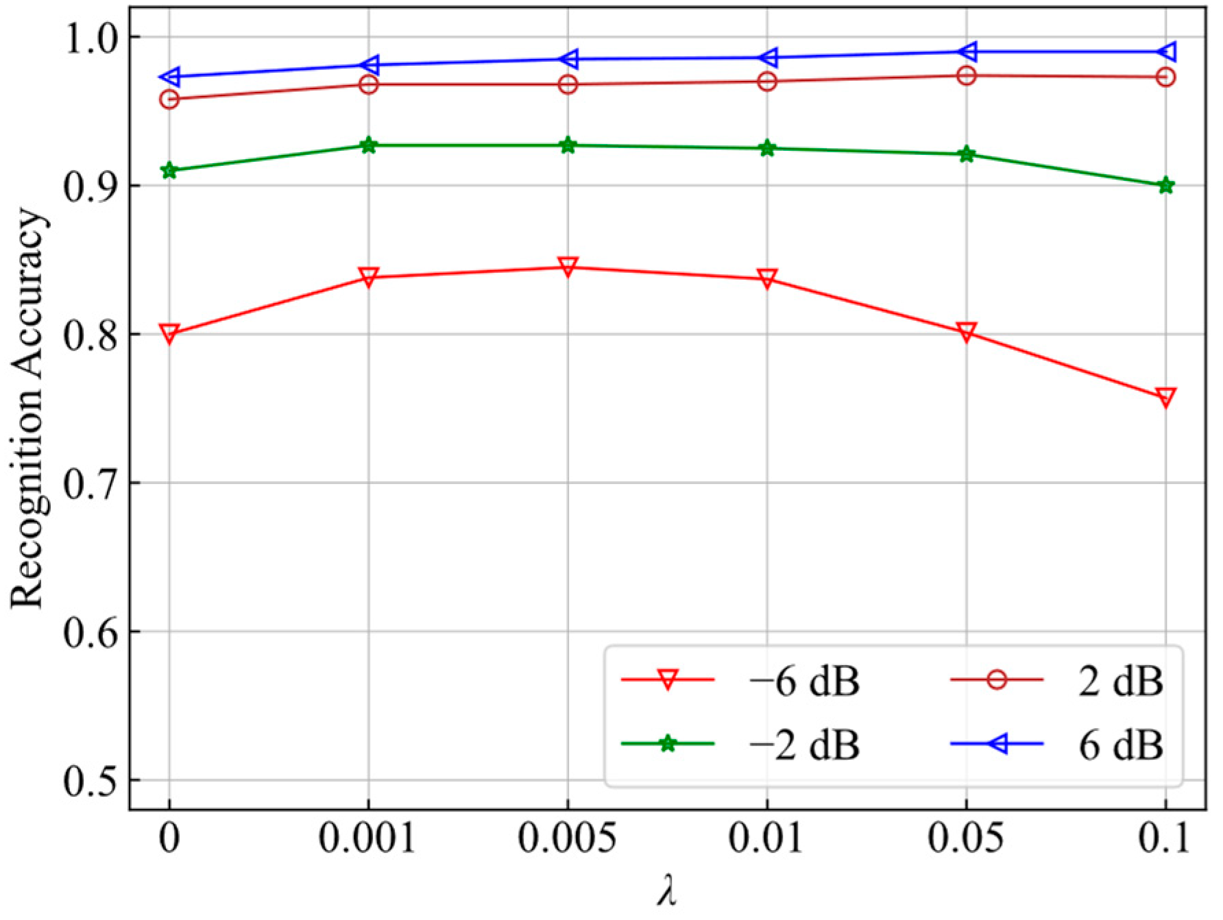
4.2. Comparison of Recognition Performance under Different Parameters

4.2.1. Comparison of Recognition Accuracy under Different Loss Functions

In this paper, for ZigBee devices and USRP 310 devices, we set $\kappa =3$ and $\kappa =5$, respectively. Meanwhile, the recognition performance was better when $r=10$ after preliminary experiments. The recognition accuracy is shown in Figure 5, corresponding to different $\lambda$ values when the SNR varied between −6 and 6 dB. It can be seen that the experimental results verified the theoretical analysis of the PL. The $\lambda$ value determined the degree of aggregation of each class, which in turn affected the distribution of the distance within and between classes, making the recognition performance vary under different $\lambda$ values. It was concluded that the recognition accuracy was the highest when $\lambda$ was about 0.005.

When $\lambda$ increased from 0, the intra-class tightness of each class gradually increased, which then expanded the inter-class distances, improving both the classification ability for known classes and the rejection ability for unknown classes. With the further increase in $\lambda$, the recognition performance tended to be stable. When $\lambda$ was too large, the feature space was excessively tightened in the training period, which resulted in overfitting. Similarly, the influence was more pronounced at a low SNR, so choosing the appropriate $\lambda$ is critical.

As shown in Figure 6, we extracted the output features of the full connection layer and drew the feature distribution maps under different $\lambda$ values. According to the analysis of feature distribution, it was concluded that DCEL could complete classification and recognition. When PL was added, the inter-class distances and the distribution of unknown space were amplified by improving the intra-class compactness, which also further separated the known and unknown classes in the feature space and improved the classification performance.

4.2.2. Comparison of Recognition Accuracy for Different r Values

Before fitting the Weibull model for each class, the distances between the correctly classified samples and the corresponding mean features during the training process needed to be sorted, and the Weibull model was fitted using the r largest distances of the samples after sorting. The $\lambda$ value was set to 0.005, and the comparison of the effect of r on the recognition performance is shown in Figure 7.

The experimental results showed that the recognition accuracy was optimal when r was 10–20, and gradually decreased when r was too large. This also verified the previous analysis of r. Fitting the Weibull model with a large number of samples of known classes increased the probability that the known classes were recognized as unknown ones.

4.2.3. Comparison of Recognition Accuracy with Different Feature Dimensions

In the training and testing process, we used the distances between the sample features and the prototypes to measure the attribution, and the dimensionality change of the features also had an impact on the recognition performance. The experiments were conducted when the other parameters were optimal. Figure 8 shows the recognition performance of the network when the feature dimensions were 2, 3, 4, and 5 and the SNR was −4 dB and 0 dB, respectively. It can be seen that using a lower feature dimension could achieve a higher recognition accuracy, and a higher feature dimension improved only the computational complexity of the network rather than the recognition performance.

As shown in Figure 8, the feature dimension had a certain impact on the recognition performance at a low SNR, and the impact became smaller at a high SNR. At the same time, according to the results of several experiments, the recognition accuracy of three-dimensional features was slightly improved compared with that of two-dimensional features. When the dimensions continued to increase, the recognition accuracy did not change significantly, but this increased the network complexity. Therefore, three-dimensional features were finally chosen for the model.

4.3. Comparison of Recognition Performance of Different Models

4.3.1. Comparison of Recognition Accuracy

The comparison of the results from the ZigBee devices is shown in Figure 9. The model in this paper is called EVT-Shuffle-SE. To verify the recognition performance of EVT-Shuffle-SE, the model was first compared with EVT-Shuffle without the SE module and EVT-SE without group convolution and channel shuffle. Then, EVT-Shuffle-SE was also compared with OpenMax [26,27], Center_Loss [29], and CPN [33]. We used the same network structure as CPN, OpenMax, and Center_Loss. It can be seen that the recognition accuracy of the model was effectively improved by introducing the attention mechanism after adding the SE module. EVT-Shuffle-SE with group convolution and channel shuffle also showed a slight improvement over EVT-SE with fewer network parameters. Meanwhile, the model proposed in this paper had an advantage over the other models at a lower SNR. When the SNR was greater than 0 dB, the recognition accuracy of our model reached more than 95%.

In Figure 10, the confusion matrix for open-set recognition is plotted at −6 dB, −2 dB, 2 dB, and 6 dB, respectively. It can be seen that device 1 and device 2 were easily confused, and device 3 was more independent. Even at a lower SNR, the signals from device 4 and device 5 were successfully rejected as an unknown class.

We also conducted experiments on the USRP 310 device. As shown in

Table 1. Comparison of recognition accuracy of different models.

Models	EVT_PN_Shuffle	OpenMax	CPN	Center_Loss
Recognition Accuracy	90.3%	85.8%	78%	81.5%

, the experimental results demonstrated that the recognition accuracy of the model still reached more than 90% for the 10 types of devices under mixed SNRs. The model also had better recognition performance.

Figure 11 shows the confusion matrix for 10 types of devices. It can be seen that the rejection rate for the three unknown devices reached 84%.

4.3.2. Comparison of Robustness

During the training process, the initialization of the networks has a severe impact on the results, and it is difficult to ensure that the network achieves optimal recognition by fixing the initial network parameters and weights.

In the CPN model, a fixed distance threshold was used to detect the unknown samples, but the distribution of the sample features changed significantly during each training process. Therefore, the test results after each training fluctuated. In this paper, we incorporated EVT to improve the classification rules. Firstly, prototypical networks and joint loss were used to make the feature space of each class more independent and separate. Meanwhile, the distance was also more suitable for measuring the attribution. Finally, the classification results were weighted and revised by the probability from the Weibull model. Thus, our algorithm effectively increased the robustness and alleviated the influence of the model using the initial parameters, SNR, and instability of the network.

As shown in Figure 12, the test results of the three models were compared after multiple experiments at −4 dB and 0 dB using the ZigBee dataset. The comparison showed that the test results of EVT-Shuffle-SE were more robust, while the CPN and OpenMax models fluctuated more. The fluctuation increased as the SNR decreased. Therefore, the recognition performance of our model was more stable.

5. Conclusions

In this paper, we combined prototypical networks and EVT to achieve open-set SEI. The SE module was added to the one-dimensional CNN to strengthen the classification ability by adjusting the channel weights. Group convolution and channel shuffle strengthened the recognition of I and Q channels, reducing the network complexity and overfitting. In addition to prototype learning, the network was trained by joint loss to complete the separation of inter-class signals and the aggregation of intra-class signals in the feature space. The Weibull models were fitted for each class with the assistance of EVT, and the joint loss function also ensured the independence of each Weibull model. Finally, the weights and Weibull CDF probability were used to revise the network outputs of the test samples, which effectively realized the open-set recognition and improved the stability. Follow-up work should further classify the unknown signals, and the modeling and analysis of these unknown signals should be enhanced.

References

1. Talbot, K.I.; Duley, P.R.; Hyatt, M.H. Specific emitter identification and verification. Technol. Rev. 2003, 113, 113–130. [Google Scholar]
2. Nouichi, D.; Abdelsalam, M.; Nasir, Q.; Abbas, S. IoT Devices security using RF fingerprinting. In Proceedings of the 2019 Advances in Science and Engineering Technology International Conferences (ASET), Dubai, United Arab Emirates, 26 March–10 April 2019; pp. 1–7. [Google Scholar]
3. Bihl, T.J.; Bauer, K.W.; Temple, M.A. Feature selection for RF fingerprinting with multiple discriminant analysis and using ZigBee device emissions. IEEE Trans. Inf. Secur. 2016, 11, 1862–1874. [Google Scholar] [CrossRef]
4. Patel, H.J.; Temple, M.A.; Baldwin, R.O. Improving ZigBee device network authentication using ensemble decision tree classifiers with radio frequency distinct native attribute fingerprinting. IEEE Trans. Rel. 2015, 64, 221–233. [Google Scholar] [CrossRef]
5. Ramsey, B.W.; Temple, M.A.; Mullins, B.E. PHY foundation for multi-factor ZigBee node authentication. In Proceedings of the 2012 IEEE Global Communications Conference (GLOBECOM), Anaheim, CA, USA, 3–7 December 2012; pp. 795–800. [Google Scholar]
6. Danev, B.; Capkun, S. Transient-based identification of wireless sensor nodes. In Proceedings of the 2009 International Conference on Information Processing in Sensor Networks, San Francisco, CA, USA, 13–16 April 2009; pp. 25–36. [Google Scholar]
7. Mohamed, I.; Dalveren, Y.; Catak, F.O.; Kara, A. On the Performance of Energy Criterion Method in Wi-Fi Transient Signal Detection. Electronics 2022, 11, 269. [Google Scholar] [CrossRef]
8. Yang, Y.S.; Guo, Y.; Li, H.G.; Sui, P. Fingerprint feature recognition of frequency hopping based on high order cumulant estimation. In Proceedings of the 2018 IEEE 3rd Advanced Information Technology, Electronic and Automation Control Conference (IAEAC), Chongqing, China, 12–14 October 2018; pp. 2175–2179. [Google Scholar]
9. Xu, S.H.; Huang, B.X.; Xu, L.N.; Xu, Z.G. Radio transmitter classification using a new method of stray features analysis combined with PCA. In Proceedings of the MILCOM 2007-IEEE Military Communications Conference, Orlando, FL, USA, 29–31 October 2007; pp. 1–5. [Google Scholar]
10. Udit, S.; Nikita, T.; Gagarin, B. Specific emitter identification based on variational mode decomposition and spectral features in single hop and relaying scenarios. IEEE Trans. Inf. Secur. 2018, 14, 581–591. [Google Scholar]
11. Lecun, Y.; Bottou, L. Gradient-Based Learning Applied to Document Recognition; IEEE: New York, NY, USA, 1998; Volume 86, pp. 2278–2324. [Google Scholar]
12. Pan, Y.W.; Yang, S.H.; Peng, H.; Li, T.Y.; Wang, W.Y. Specific emitter identification based on deep residual networks. IEEE Access 2019, 7, 54425–54434. [Google Scholar] [CrossRef]
13. Peng, L.N.; Zhang, J.Q.; Liu, M.; Hu, A.Q. Deep learning based RF fingerprint identification using Differential Constellation Trace Figure. IEEE Trans. Veh. Technol. 2019, 69, 1091–1095. [Google Scholar] [CrossRef]
14. Ding, L.D.; Wang, S.L.; Wang, F.G.; Zhang, W. Specific emitter identification via convolutional neural networks. IEEE Commun. Lett. 2018, 22, 2591–2594. [Google Scholar] [CrossRef]
15. Chen, Y.; Chen, X.; Lei, Y. Emitter Identification of Digital Modulation Transmitter Based on Nonlinearity and Modulation Distortion of Power Amplifier. Sensors 2021, 21, 4362. [Google Scholar] [CrossRef]
16. Merchant, K.; Revay, S.; Stantchev, G.; Nousain, B. Deep learning for RF device fingerprinting in cognitive communication networks. IEEE J. Sel. Top. Signal Process. 2018, 12, 160–167. [Google Scholar] [CrossRef]
17. Sankhe, K.; Belgiovine, M.; Zhou, F.; Angioloni, L.; Restuccia, F.; D’Oro, S.; Melodia, T.; Ioannidis, S.; Chowdhury, K. No Radio Left Behind: Radio fingerprinting through deep learning of Physical-Layer hardware impairments. IEEE Trans. Cogn. Commun. Netw. 2019, 6, 165–178. [Google Scholar] [CrossRef]
18. Qing, G.W.; Wang, H.F.; Zhang, T.P. Radio frequency fingerprinting identification for Zigbee via lightweight CNN. Phys. Commun. 2021, 44, 101250. [Google Scholar] [CrossRef]
19. Liu, Y.H.; Xu, H.; Qi, Z.S.; Shi, Y.H. Specific emitter identification against unreliable features interference based on Time-Series classification network structure. IEEE Access 2020, 8, 200194–200208. [Google Scholar] [CrossRef]
20. Wang, Y.; Gui, G.; Gacanin, H.; Ohtsuki, T.; Dobre, O.A.; Poor, H.V. An efficient specific emitter identification method based on Complex-Valued neural networks and network compression. IEEE J. Sel. Areas Commun. 2021, 39, 2305–2317. [Google Scholar] [CrossRef]
21. Xing, C.; Zhou, Y.; Peng, Y.; Hao, J.; Li, S. Specific Emitter Identification Based on Ensemble Neural Network and Signal Graph. Appl. Sci. 2022, 12, 5496. [Google Scholar] [CrossRef]
22. Gutierrez del Arroyo, J.A.; Borghetti, B.J.; Temple, M.A. Considerations for Radio Frequency Fingerprinting across Multiple Frequency Channels. Sensors 2022, 22, 2111. [Google Scholar] [CrossRef] [PubMed]
23. Tian, Q.; Lin, Y.; Guo, X.; Wang, J.; AlFarraj, O.; Tolba, A. An Identity Authentication Method of a MIoT Device Based on Radio Frequency (RF) Fingerprint Technology. Sensors 2020, 20, 1213. [Google Scholar] [CrossRef] [PubMed] [Green Version]
24. Chen, S.; Wen, H.; Wu, J.; Xu, A.; Jiang, Y.; Song, H.; Chen, Y. Radio Frequency Fingerprint-Based Intelligent Mobile Edge Computing for Internet of Things Authentication. Sensors 2019, 19, 3610. [Google Scholar] [CrossRef] [PubMed] [Green Version]
25. Aneja, S.; Aneja, N.; Bhargava, B.; Chowdhury, R.R. Device fingerprinting using deep convolutional neural networks. Int. J. Comm. Netw. Distr. Syst. 2022, 28, 171–198. [Google Scholar] [CrossRef]
26. Hanna, S.; Karunaratne, S.; Cabric, D. Open set wireless transmitter authorization: Deep learning approaches and dataset considerations. IEEE Trans. Cogn. Commun. Netw. 2021, 7, 59–72. [Google Scholar] [CrossRef]
27. Chen, W.; Wang, Y.H.; Song, J.; Li, Y. Open set HRRP recognition based on convolutional neural network. J. Eng. 2019, 2019, 7701–7704. [Google Scholar] [CrossRef]
28. Bendale, A.; Boult, T. Towards open set deep networks. In Proceedings of the IEEE Conference on Computer Vision and Pattern Recognition (CVPR), Las Vegas, NV, USA, 26 June–1 July 2016; pp. 1563–1572. [Google Scholar]
29. Wen, Y.; Zhang, K.; Li, Z.; Qiao, Y. A Discriminative Feature Learning Approach for Deep Face Recognition. In European Conference on Computer Vision; Springer: Berlin/Heidelberg, Germany, 2016; pp. 499–515. [Google Scholar]
30. Draganov, A.; Brown, C.; Mattei, E.; Dalton, C.; Ranjit, J. Open set recognition through unsupervised and class-distance learning. In 2nd ACM Workshop on Wireless Security and Machine Learning; ACM: New York, NY, USA, 2020; pp. 7–12. [Google Scholar]
31. Snell, J.; Swersky, K.; Zemel, R.S. Prototypical networks for few-shot learning. arXiv 2017, arXiv:1703.05175. [Google Scholar]
32. Yang, H.M.; Zhang, X.Y.; Yin, F.; Liu, C.L. Robust classification with convolutional prototype learning. In Proceedings of the IEEE Conference on Computer Vision and Pattern Recognition, Salt Lake City, UT, USA, 18–23 June 2018; pp. 3474–3482. [Google Scholar]
33. Yang, H.M.; Zhang, X.Y.; Yin, F.; Yang, Q.; Liu, C.L. Convolutional prototype network for open set recognition. IEEE Trans. Pattern Anal. Mach. Intell. 2020, 44, 2358–2370. [Google Scholar] [CrossRef] [PubMed]
34. Liu, C.L.; Nakagawa, M. Evaluation of prototype learning algorithms for nearest-neighbor classifier in application to handwritten character recognition. Pattern Recognit. 2001, 34, 601–615. [Google Scholar] [CrossRef]
35. Fisher, R.A.; Tippett, L.H.C. Limiting forms of the frequency distribution of the largest or smallest member of a sample. In Mathematical Proceedings of the Cambridge Philosophical Society; Cambridge University Press: Cambridge, UK, 1928; Volume 24, pp. 180–190. [Google Scholar]
36. Scheirer, W.J.; Rocha, A.R.; Micheals, R.J.; Boult, T.E. Meta-recognition: The theory and practice of recognition score analysis. IEEE Trans. Pattern Anal. Mach. Intell. 2011, 33, 1689–1695. [Google Scholar] [CrossRef]
37. Hu, J.; Shen, L.; Albanie, S.; Albanie, S.; Wu, E.H. Squeeze-and-excitation networks. IEEE Trans. Pattern Anal. Mach. Intell. 2020, 42, 2011–2023. [Google Scholar] [CrossRef] [Green Version]
38. Zhang, X.Y.; Zhou, X.Y.; Lin, M.X.; Sun, J. ShuffleNet: An extremely efficient convolutional neural network for mobile devices. In Proceedings of the IEEE Conference on Computer Vision and Pattern Recognition, Salt Lake City, UT, USA, 18–23 June 2018; pp. 6848–6856. [Google Scholar]
39. Kingma, D.P.; Ba, J. Adam: A Method for Stochastic Optimization. In Proceedings of the International Conference on Learning Representations, San Diego, CA, USA, 7–9 May 2015. [Google Scholar]
Figure 1. Open-set recognition model based on prototypical networks and EVT.
Applsci 13 03878 g001
Figure 2. The network structure for open-set recognition.
Applsci 13 03878 g002
Figure 3. Schematic of group convolution and channel shuffle.
Applsci 13 03878 g003
Figure 4. One-dimensional SE model.
Applsci 13 03878 g004
Figure 5. Comparison of recognition accuracy for different values of λ .
Applsci 13 03878 g005
Figure 6. Feature distribution under different values of λ : (a) training features when λ was 0; (b) testing features when λ was 0; (c) training features when λ was 0.005; (d) testing features when λ was 0.005.
Applsci 13 03878 g006
Figure 7. Comparison of recognition accuracy for different r values.
Applsci 13 03878 g007
Figure 8. Comparison of recognition accuracy with different feature dimensions.
Applsci 13 03878 g008
Figure 9. Comparison of recognition accuracy of different models: (a) comparison under different modules; (b) comparison with other models.
Applsci 13 03878 g009
Figure 10. Confusion matrix under different SNRs: (a) confusion matrix at −6 dB; (b) confusion matrix at −2 dB; (c) confusion matrix at 2 dB; (d) confusion matrix at 6 dB.
Applsci 13 03878 g010
Figure 11. Confusion matrix under mixed SNRs of −4–10 dB.
Applsci 13 03878 g011
Figure 12. Robustness comparison of different models: (a) ours model; (b) CPN; (c) OpenMax.
Applsci 13 03878 g012