Armature Electromagnetic Force Extrapolation Prediction Method for Electromagnetic Railgun at High Speed

Abstract

The analysis and calculation of the armature electromagnetic force is the premise of studying the dynamic characteristics of the electromagnetic railgun. Aiming at the problem of the numerical solution “pseudo-oscillation” at high speed, an extrapolation prediction method of armature electromagnetic force based on the Deep Belief Network-Deep Neural Network (DBN-DNN) is proposed. Firstly, the electromagnetic field control equation and armature dynamics equation, considering the influence of armature movement, are given, and the finite element simulation model of the electromagnetic railgun is established to analyze the dynamic characteristics and numerical solution stability of the armature electromagnetic force. Then, based on the stable numerical simulation data under different armature conductivities, a DBN-DNN method is proposed to realize the extrapolation prediction of the armature electromagnetic force under the standard conductance. Finally, the extrapolation prediction performance of the proposed method is tested by two electromagnetic railgun cases. Additionally, we further propose the training strategy of DBN-DNN parameters from solving armature electromagnetic force at low conductivity to standard conductivity. The armature electromagnetic force extrapolation prediction method for the whole launch process from low speed to high speed provides a new idea for the dynamic characteristic analysis of the high-speed electromagnetic railgun.

1. Introduction

As a subversive launcher, the electromagnetic railgun is an important support for the country’s major strategic needs. The armature electromagnetic force is one of the basic parameters in the launching process of the electromagnetic railgun. The systematic analysis of armature electromagnetic force is of great significance to the research on the dynamic characteristics and reliability design of electromagnetic railgun.

The numerical simulation method is an indispensable tool in the characteristic analysis, and domestic and foreign research teams have used different methods to carry out numerical simulation research on the electromagnetic railgun. References [1,2] used Maxwell and ANSYS software to simulate and analyze the electromagnetic railgun, and the research conclusions obtained had a certain guiding significance, but the influence of the armature movement was not considered. References [3,4,5,6] used MEGA and COMSOL software to study the electromagnetic field distribution characteristics considering the influence of armature movement in a 2D model, but they did not analyze the 3D model, which leads to inequality with the actual model. References [7,8,9,10,11] used different numerical simulation methods to establish a 3D model of the electromagnetic railgun considering the influence of armature movement, and they simulated the field distribution, emission characteristics, frictional wear, and armature movement characteristics. Among them, the reference [7] used the controlled diffusion equation method, which considered the effects of armature movement by adding a velocity term to the electromagnetic field control equation. The velocity was reflected in the convection term of the equation, and the Peclet number (P_e) would increase as the velocity increased, and when P_e > 1, the numerical solution “pseudo-oscillation” may occur. Additionally, this restricted stable numerical simulation at high speeds. References [8,9,10] used the moving mesh method, which caused the convection term to not appear explicitly in the equation, but the velocity was reflected in the discrete mesh of the moving body at each time step. However, due to the linkage relationship between the armature position and grid change, the inversion and quality degradation of the grid at a high speed made the calculation difficult to converge, and there was a grid mismatch problem on the interface of the relative motion area. Reference [11] used the arbitrary Lagrangian–Euler method, and although the numerical simulation of electromagnetic railguns at high speed could be realized, due to the problems of angles, points, and edges in the coupling method, the calculation error was large.

The numerical simulation at high speed still has the problems of poor accuracy, difficult calculation, or even impossible calculation, and it is difficult or even impossible to achieve the accurate calculation solution of a high-speed electromagnetic railgun through the numerical simulation method alone. In recent years, AI technology has developed rapidly. Deep learning is an important method of data processing in AI. It can use flexible network structures and efficient optimization algorithms to obtain a strong representation and generalization ability for high-dimensional and nonlinear problems. Deep learning can learn the historical characteristics of numerical simulation results to predict and directly generate numerical simulation results, which has a great development potential. Reference [12] used Deep Belief Networks (DBN) to establish a cogging torque prediction and analysis model for permanent magnet synchronous motors, and the feasibility of the deep learning prediction model is verified by computational examples. Reference [13] proposed a deep neural network method aiming at the problem that traditional numerical simulation methods are computationally intensive and difficult to achieve a balance between accuracy and efficiency, which realized the rapid prediction of aerodynamic noise under the premise of maintaining accuracy. Reference [14] established a rapid calculation method of force based on Deep Neural Networks (DNN) that aimed at the difficult problem of modeling ironless permanent magnet synchronous linear motors and provided a high-precision and high-efficiency model for global optimization of motor parameters. The combination of numerical simulation and deep learning technology has attracted the attention of scholars in recent years and has led to some achievements in electromagnetics. Reference [15] used numerical simulation data and Convolutional Neural Networks (CNN) to predict two-dimensional potential distributions, and the prediction error was less than 1%. Reference [16] trained CNN in a supervised manner and learned the mapping of coils to motor magnetic field distributions, and the result showed good accuracy in magnetic field prediction. Reference [17] proposed a sequence-based modular network and an end-to-end network to predict the motor drive efficiency maps, which showed good accuracy in prediction. However, in the field of electromagnetic rail launch, there is a lack of application research combining numerical simulation and deep learning technology.

This paper combines the numerical simulation data of the electromagnetic railgun with depth learning and proposes an extrapolation prediction method of the armature electromagnetic force using the DBN-DNN model. This paper is organized as follows: Section 2 presents the governing equation, which considering the influence of armature movement, then establishes the finite element simulation model to analyze the dynamic characteristics and numerical solution stability of the armature electromagnetic force under different conductivity. Section 3 aims at the “pseudo-oscillation” problem of the numerical solution at high speed affected by P_e, proposes an extrapolation prediction method of armature electromagnetic force with standard armature conductivity, and then describes the network architecture and working principle of DBN-DNN. Section 4 uses two electromagnetic railgun cases to test the extrapolation prediction performance of the model and further proposes the acceleration effect of DBN-DNN model parameters when solving low conductivity transfer to standard conductivity, which improves the training efficiency of the model.

2. Numerical Simulation of Armature Electromagnetic Force

In the governing equation of the electromagnetic railgun and the finite element numerical simulation, the following assumptions are made:

• The rail is in good contact with the armature, ignoring the unevenness of the contact interface and material wear.
• The generation of molten aluminum at the interface during the launch will sharply reduce the sliding friction coefficient and tend to stabilize in order to simplify the calculation; it is assumed that it remains at a constant value of 0.11 throughout the launch process [18].
• The performance parameters of armature and rail materials (such as conductivity and relative permeability) are constant values during numerical simulation, and they do not change with time and temperature.

2.1. Governing Equation

The Maxwell equations, the constitutive equation, and the A-φ potential function are combined while considering the influence of the armature movement, and then the Coulomb specification is introduced. The electromagnetic field governing equation [19,20] described in stationary reference frame is obtained

$$\left\{\begin{array}{l}\nabla \times \left(\frac{1}{\mu }\nabla \times \mathit{A}\right)+\sigma \nabla \varphi +\sigma \frac{\partial \mathit{A}}{\partial t}-\sigma \mathit{v}\times \nabla \times \mathit{A}=0\\ \nabla \times \left(\sigma \nabla \varphi +\sigma \frac{\partial \mathit{A}}{\partial t}-\sigma \mathit{v}\times \nabla \times \mathit{A}\right)=0\end{array}\right.$$

(1)

In the formula, A is the magnetic vector potential, φ is the electrical scalar potential, μ, σ, and v denote a partition function, namely, μ is the permeability, σ is the electrical conductivity, and v is the velocity, respectively. In the armature area: μ = μ_a, σ = σ_a, and v ≠ 0; in the rail area: μ = μ_r, σ = σ_r, and v = 0; in the air area: μ = μ₀ = 4π × 10⁻⁷ H/m, σ = σ₀, and v = 0.

Then, the armature electromagnetic force F_em is

$${\mathit{F}}_{\mathrm{em}}={\displaystyle {\mathrm{\iiint }}_{\mathrm{\Omega }}\mathit{J}\times \mathit{B}\mathrm{d}V}$$

(2)

In the formula, J is the current density; B is the magnetic flux density. Under the combined action of the armature electromagnetic force F_em, the armature rail friction F_f, and the air resistance F_air, the kinetic equation [21] are

$$\begin{array}{l}{m}_{\mathit{a}}\mathit{a}=F_{\mathrm{em}}-F_f-F_{\mathrm{air}}\\ \hspace{1em}\hspace{0.33em}\hspace{0.33em}\hspace{0.17em}={\displaystyle {\mathrm{\iiint }}_{\mathrm{\Omega }}\mathit{J}\times \mathit{B}\mathrm{d}V}-{\mu }_f\left(F_{\mathrm{N},\mathrm{em}}+F_{\mathrm{N},\mathrm{p}}\right)-\frac{\mathit{\gamma }+1}{2}{\rho }_0\left(S{v}^2+Sx\mathit{a}+\frac{C_{f}L{v}^{2}x}{2}\right)\end{array}$$

(3)

In the formula, m_a, a, and x are the mass, acceleration, and displacement of armature, respectively; μ_f is the friction coefficient; F_N,em is the electromagnetic contact pressure; F_N,p is the mechanical preloading pressure; γ is the specific heat ratio of the air; ρ₀ is the initial air density; S is the armature cross-sectional area; L is the perimeter of armature section; and C_f is the viscous friction coefficient.

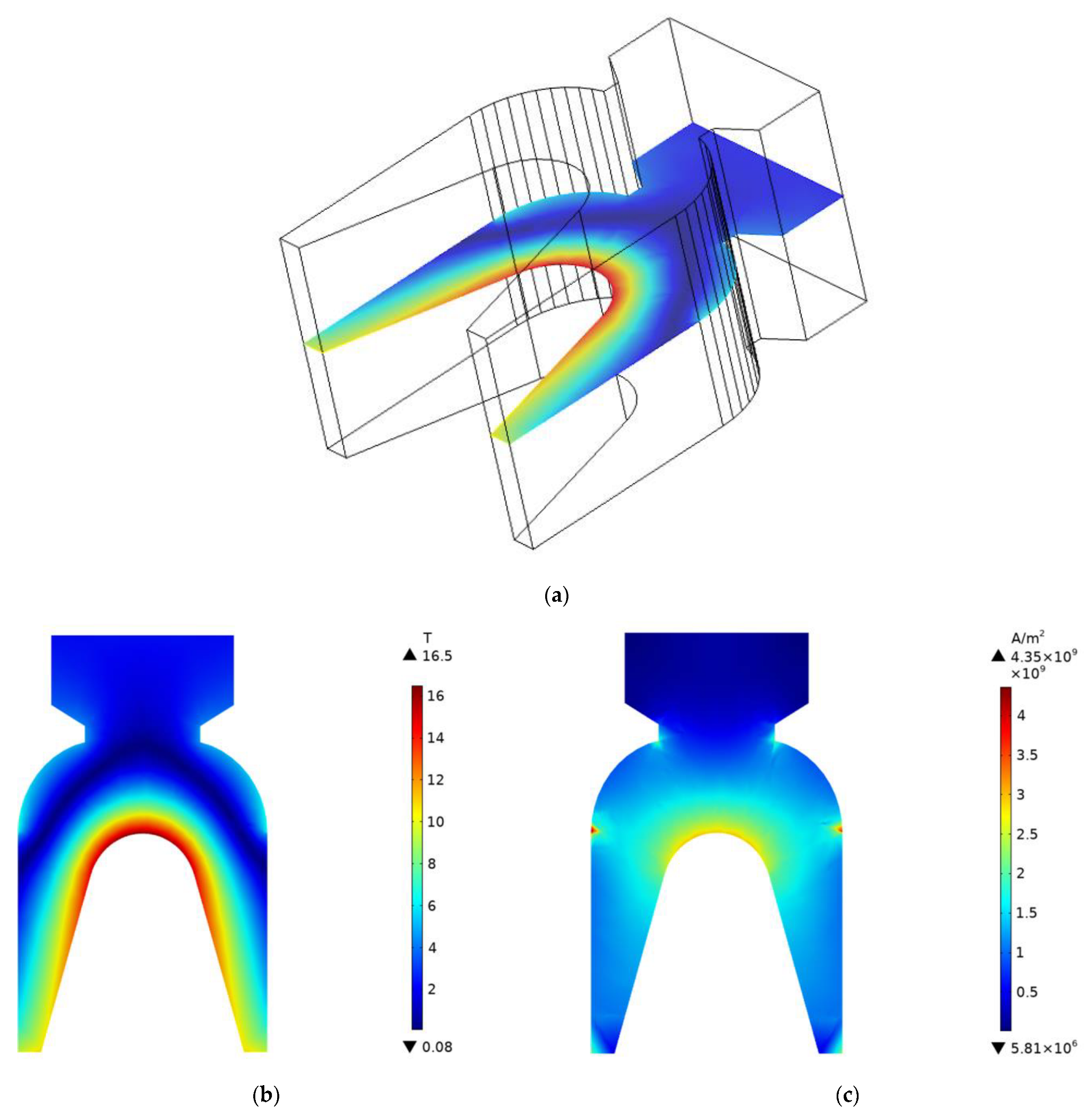
2.2. Finite Element Model

The typical C-shaped armature and the 30 mm × 30 mm rectangular caliber electromagnetic railgun are taken as the research objects. Based on the COMSOL finite element simulation software, the armature electromagnetic force is simulated and analyzed. The armature and rail model parameters are shown in

Table 1. Parameters of armature and rail model.

Model Parameters	Symbol	Values
Rail length/mm	lr	3500.00
Rail height/mm	hr	40.00
Rail width/mm	wr	20.00
Rail conductivity/(S/m)	σr	3.45 × 107
Rail permeability/(H/m)	μr	4π × 10−7
Armature length/mm	la	50.00
Armature height/mm	ha	28.00
Armature width/mm	wa	30.00
Armature conductivity/(S/m)	σa	2.20 × 107
Armature permeability/(H/m)	μa	4π × 10−7

.

The electromagnetic railgun geometric model and the mesh segmentation result are shown in Figure 1. Among them, the air region and some rail regions are not drawn. Considering the distribution characteristics of the electromagnetic field, the mesh of the rail is divided into cuboid shapes that gradually thicken from the inside to the outside and the mesh of the C-shaped armature is divided into hexahedral shapes with relatively regular regularities through the operations of “mapping”, “distribution”, “sweeping”, “free quadrilateral grid”, and “size”. The air area is divided using a “free tetrahedral” grid. Through the above meshing operation, the average element mass of the armature and rail areas is 0.9171, and the average element mass of the entire model area is 0.9119. The closer this value is to 1, the better the mesh quality.

In order to observe the change in electromagnetic force more clearly with the excitation current, the trapezoidal excitation current is used closely to the project (constant current at the maximum current), as shown in Figure 2. The excitation current flows from the lower face of rail A in Figure 1, flows through the armature, and then flows out of the lower face of rail B.

The material properties of the electromagnetic railgun are defined in the finite element simulation software based on Table 1. In this paper, the controlled diffusion equation method is used to numerically simulate the electromagnetic railgun, and the specific setting method is as follows: Setting the conditions for the physics fields of the “current” and “magnetic field”, and then adding velocity terms by modifying the electromagnetic field control equation. The armature velocity is calculated using the physics field of “global ordinary differential and differential algebraic equations”, and then so are the values of the relevant parameters in the kinetic equation, as shown in

Table 2. Parameters of armature kinetic equation.

Parameters	Symbol	Values
Armature mass/g	ma	125.00
Friction coefficient	μ	0.11
Mechanical preloading pressure/N	FN,p	5600
Specific heat ratio of the air	γ	1.4
Initial air density/(kg/m3)	ρ0	1.29
Armature cross-sectional area/m2	S	0.00084
Perimeter of armature section/m	L	0.116
Viscous friction coefficient	Cf	0.003

. During transient solving, we use the backward difference scheme in time. In the backward difference scheme, the equations are evaluated at the current time; therefore, it is an implicit scheme.

2.3. Dynamic Characteristics and Numerical Solution Stability of Armature Electromagnetic Force

The armature electromagnetic force and movement velocity obtained by numerical simulation are shown in Figure 3. Before the armature velocity reaches 500 m/s, the stable calculation of the armature electromagnetic force and velocity can be realized; when the armature velocity increases to 500 m/s, the calculated values of the armature electromagnetic force and velocity begin to become unstable, that is, the “pseudo-oscillation” problem of the numerical solution occurs.

The numerical simulation results of the electromagnetic field on the rail section at 1.2 ms are shown in Figure 4. The rail section at 10 mm from the tail of the armature is selected as the observation angle. Under the joint action of the skin effect, proximity effect, and velocity skin effect, the magnetic flux density tends to be concentrated on the inner surface of the rail with a maximum value of 8.61 T, and the current density tends to be concentrated at two sharp corners of the inner surface of the rail, and the maximum current density is 8.84 × 10⁸ A/m².

The numerical simulation results of the electromagnetic field on the armature horizontal cross-section at 1.2 ms are shown in Figure 5. The horizontal cross-section in the middle of the armature is selected as the observation angle. The magnetic flux density tends to be concentrated at the throat position inside the armature with a maximum value of 16.5 T; the current density tends to be concentrated in the inner throat and outer fillet position of the armature, and the maximum current density occurs at the armature outer fillet position of 4.35 × 10⁹ A/m².

The electromagnetic field governing Equation (1) of the 3D electromagnetic railgun is the convection–diffusion equation, and the velocity is reflected in the convection term of the equation. P_e is the dimensionless number that reflects the stability of the numerical solution of this equation. Additionally, the P_e is calculated as

$$P_e=\frac{convection rate}{diffusion rate}=h_c\times \frac{\sigma v}{\raisebox{1ex}{$1$}\!\left/ \!\raisebox{-1ex}{$\mu $}\right.}=h_c\sigma v\mu$$

(4)

In the formula, h_c is the cell grid size. From Equation (3), we can know that P_e is proportional to the cell grid size, velocity, conductivity, and relative permeability. When v = 500 m/s, for h_c = 7 × 10⁻⁵ in the armature region, P_e = 0.97 is calculated based on the material properties of the armature in Table 1. With the increase in velocity, the effect of the convection term is enhanced, and the P_e number increases gradually. When v > 500 m/s and P_e begins to be greater than 1, the characteristics of the “principal component dominance” of the matrix of discrete equations will be weakened [22], which leads to the morbid state of the matrix and the “pseudo-oscillation” of the numerical solution, which does not exist in physics. To avoid the problem of “pseudo-oscillation” in the numerical solution, very fine meshing must be used. Under many conditions of high speed, high relative permeability, and high conductivity, the mesh component with P_e less than 1 makes the calculation too large, and the consumption of the computer resources is too high, so it is not desirable in practice.

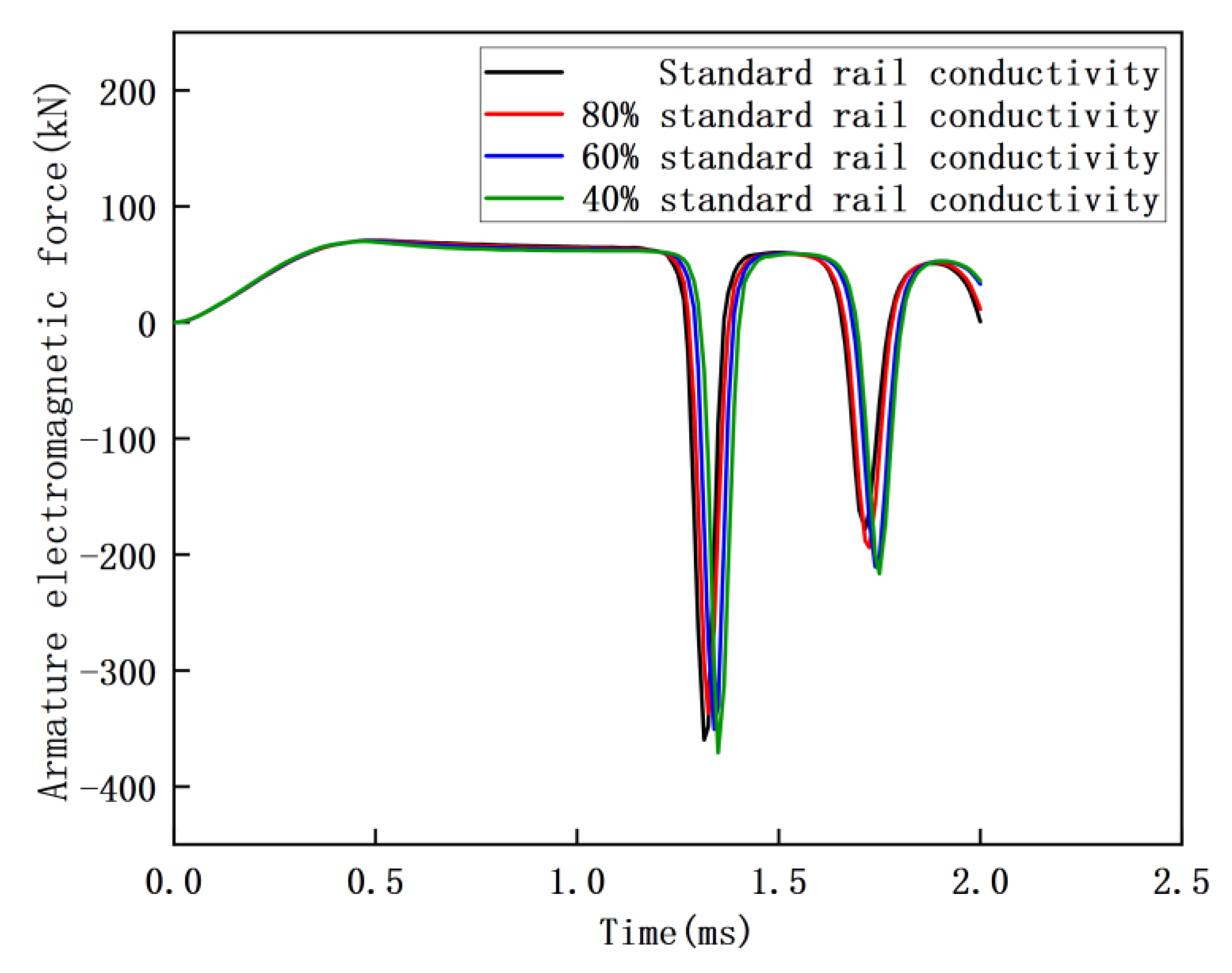
2.4. Electromagnetic Force with Different Conductivity

Electrical conductivity is one of the factors that affect P_e, and it also affects the stability of the numerical solution. Additionally, deep learning requires the armature electromagnetic force sample data under different conductivities; under a low conductivity, the electromagnetic railgun model has low computational costs and high computational efficiencies, and we find that the armature electromagnetic force at room temperature conductivity is closer to reality by comparing the calculation results under different conductivities. Therefore, taking the rail conductivity (3.45 × 10⁷ S/m) and armature conductivity (2.20 × 10⁷ S/m) at room temperature as the standards for numerical simulation, the dynamic characteristics of the armature electromagnetic force at 100%, 80%, 60%, and 40% standard conductivity are analyzed.

When the armature conductivity is always the standard conductivity and only the rail conductivity changes, the armature electromagnetic force is calculated, as shown in Figure 6. The “pseudo-oscillation” of the numerical solution appears under a different rail conductivity, and the occurrence time is basically the same. The reason for this is that the rail region is stationary, and its governing equation is the diffusion equation without convection term. P_e exists in the convection–diffusion equation, so the change in the rail conductivity will not affect the stability of the numerical solution.

When the rail conductivity is always the standard conductivity and only the armature conductivity changes, the armature electromagnetic force is calculated, as shown in Figure 7. The governing equation of the moving armature region is the convection–diffusion equation. In the process of increasing the velocity, the lower the armature conductivity, the slower P_e of the element increases, and the later the “pseudo-oscillation” of the numerical solution appears. In the case of a 40% standard armature conductivity, the stable numerical simulation of the whole launch process can be realized.

The critical velocity of the numerical simulation can be stabilized under a different armature conductivity, as shown in

Table 3. Critical velocity for stable numerical simulation at different armature conductivities.

Armature Conductivities	Critical Velocity/(m/s)
Standard armature conductivity	503.86
80% standard armature conductivity	637.01
60% standard armature conductivity	823.30
40% standard armature conductivity	956.49

. Under the standard armature conductivity, the critical velocity that can stabilize the numerical simulation is 503.86 m/s. The lower the conductivity, the greater the critical velocity of the stable numerical simulation. At a 40% standard armature conductivity, the critical velocity of the stable numerical simulation increases to 956.49 m/s.

3. The Extrapolation Prediction Method

3.1. The Extrapolation Prediction Method Flow

Aiming at the problem of “pseudo-oscillation” of the numerical solution at high speed, the numerical simulation data under a different conductivity and DBN-DNN are used to realize the extrapolation prediction of the armature electromagnetic force in the stage of “pseudo-oscillation” under a standard conductivity. The extrapolation prediction method flow is shown in Figure 8.

• The armature electromagnetic force under a different conductivity is numerically simulated. According to the stability of the numerical solution, the numerical solution is divided into the stable stage and the “pseudo-oscillation” stage.
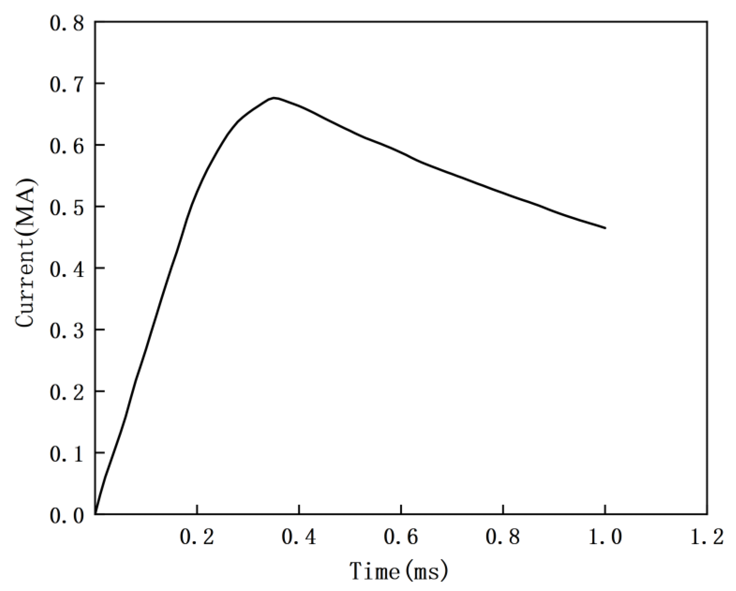
• For the stable stage, the simulation value of the armature electromagnetic force is extracted, and the sample data including the excitation current, time, velocity, armature conductivity, and electromagnetic force are obtained.
• For the “pseudo-oscillation” stage, the sample data obtained from the stability calculation stage under a different armature conductivity are used to train the DBN-DNN model with a good effect of the feature extraction and data prediction, and then the model prediction is used to obtain the extrapolation prediction value of the armature electromagnetic force of the “pseudo-oscillation” stage under the standard armature conductivity.
• For the comprehensive armature electromagnetic force of the whole launch process, the standard armature conductivity is obtained by superimposing the simulation value of the stability stage and the extrapolation prediction value of the “pseudo-oscillation” stage.

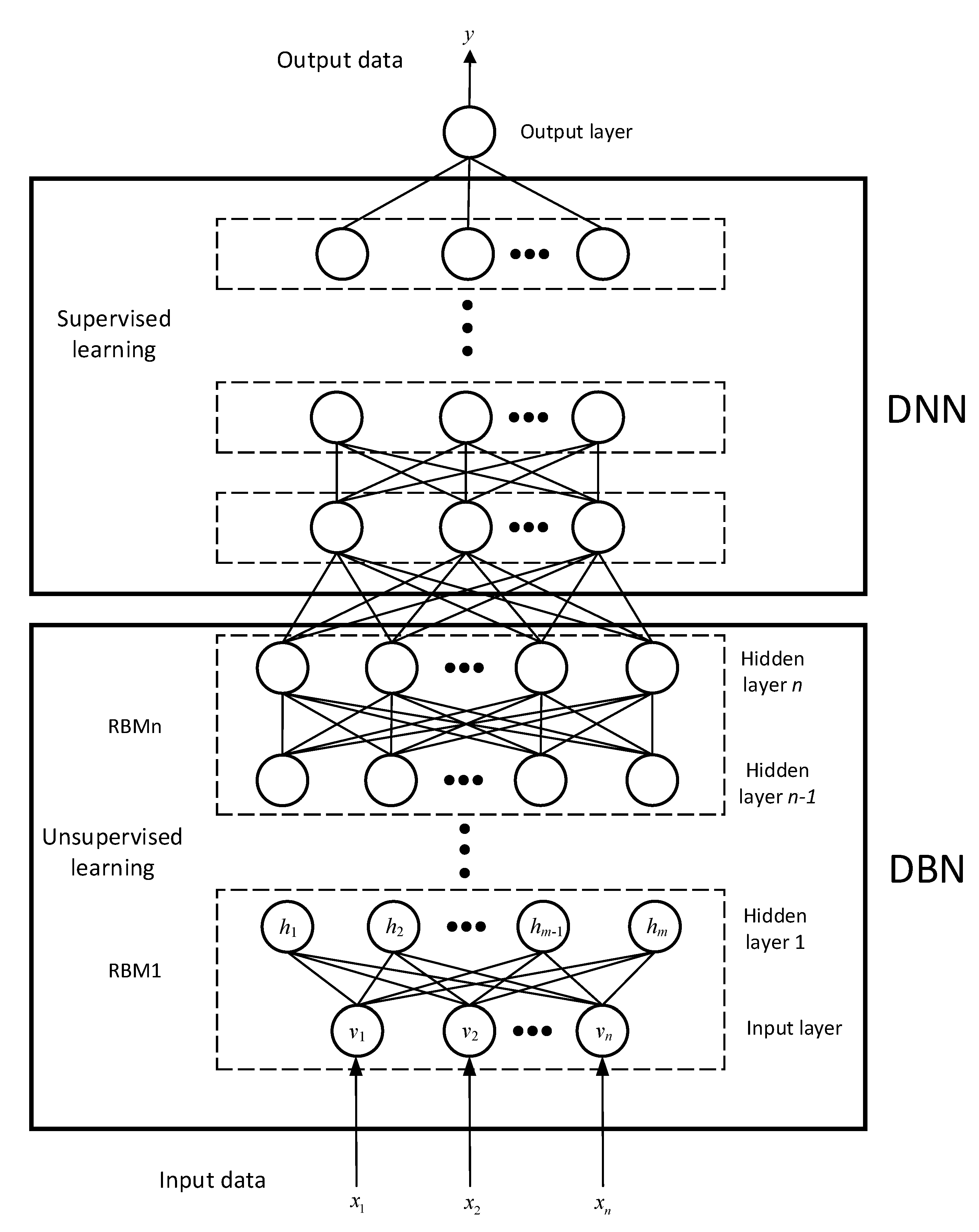
3.2. DBN-DNN

DBN-DNN does not need to establish the exact expression of the relationship between input and output. It can obtain the complex nonlinear mapping relationship between input and output through a lot of learning. It has the ability to express the data characteristics layer by layer and then deeply mine the data value. The DBN-DNN structure is shown in Figure 9. DBN-DNN is composed of DBN and DNN. Firstly, the whole DBN is initialized by a greedy unsupervised learning algorithm. After layer-by-layer training, the abstract feature vector learned by DBN is used as the input of DNN, which enables the network to be trained quickly, efficiently, stably, and reliably. Finally, the BP algorithm is used to train a DNN supervised to fit the label data.

DBN consists of multiple stacked Restricted Boltzmann Machine (RBM) units; each RBM consists of a visible layer and a hidden layer, and the neurons of the visible layer and the hidden layer are fully connected in both directions. The RBM is an energy model where the energy function is defined as E_θ(v,h) for a set of state quantities (v,h), and the joint probability distribution of the hidden layer and the visible layer is defined as P(v,h).

$$\left\{\begin{array}{l}{E}_{\theta }(v,h)=-{\displaystyle {\displaystyle \sum }_{i=1}^n}{\mathit{a}}_i{v}_i-{\displaystyle {\displaystyle \sum }_{\mathit{j}=1}^m}{\mathit{b}}_{\mathit{j}}{h}_{\mathit{j}}-{\displaystyle {\displaystyle \sum }_{i=1}^n}{\displaystyle {\displaystyle \sum }_{\mathit{j}=1}^m}{v}_i{w}_{i\mathit{j}}{h}_{\mathit{j}}\hfill \\ P(v,h)=\frac{1}{Z_{\theta }}{e}^{-E_{\theta }(v,h)}\hfill \end{array}\right.$$

(5)

In the formula, v_i and h_j are the state vectors of the visible layer and the hidden layer, respectively; a_i and b_j are the bias vectors of the visible layer and the hidden layer, respectively; n and m are the units number of the visible layer and the hidden layer, respectively; w_ij is the weight between v_i and h_j; θ = (a_i, w_ij, b_j) is the parameters of the model; and Z_θ is the normalization coefficient.

The states of the visible and hidden layer neurons of the RBM are conditionally independent, and the probability of each neuron taking the value condition is calculated as

$$\left\{\begin{array}{l}P(h_{\mathit{j}}=1|v)=\sigma ({\mathit{b}}_{\mathit{j}}+{\displaystyle {\displaystyle \sum }_{i=1}^n}{v}_i{w}_{i\mathit{j}})\hfill \\ P(v_i=1|h)=\sigma ({\mathit{a}}_i+{\displaystyle {\displaystyle \sum }_{\mathit{j}=1}^m}{w}_{i\mathit{j}}{h}_{\mathit{j}})\hfill \end{array}\right.$$

(6)

In the formula, σ(·) is the activation function. In this paper, ReLU is used as the activation function, which can overcome the gradient disappearance and retain data information very well. On the other hand, it makes the network sparse, alleviating the overfitting problem.

In this paper, the network parameters are adjusted by the maximum likelihood estimation method, so the goal of training the RBM is to maximize the likelihood function L(θ) of the network to obtain the parameter θ, that is

$$L(\theta ,v)={\displaystyle \prod _{i=1}^{n}p(v^i)}$$

(7)

To simplify the calculation, it can be written in the logarithmic form shown in Equation (8). Additionally, the Contrasting Divergence (CD) algorithm [23] is used to train the RBM.

$$\left\{\begin{array}{l}\mathrm{l}\mathrm{n}L(\theta ,v)={\displaystyle \sum _{i=1}^n\ln p(v^i)}\\ \theta =\arg \max L(\theta )=\arg \max {\displaystyle \sum _{i=1}^{n}p(v^i)}\end{array}\right.$$

(8)

In this paper, in the study of the electromagnetic railgun, the armature electromagnetic force is the output variable, and the excitation current, time, velocity, and armature conductivity, which affect the armature electromagnetic force, are the input variables. The armature electromagnetic force and its influence parameters obtained by numerical simulation are used to train the DBN-DNN, so that the DBN-DNN can learn the complex nonlinear mapping relationship to realize the extrapolation prediction of the armature electromagnetic force in the stage of “pseudo-oscillation”. When setting the network structure, the number of hidden layers is selected as four. The number of neurons in each layer is 24, 18, 14, and 10, and the training process uses the Adaptive Moment Estimation (Adam) optimizer. To reduce the complexity of the neural networks, a dropout layer has been added. On the one hand, it can simplify the structure of the neural network and reduce the training time; on the other hand, each neuron appears with a certain probability, and a weight update no longer depends on the joint action of fixed relationship neurons, thereby improving the overfitting phenomenon of the network.

4. Case Analysis

Two cases of electromagnetic railguns with different exit velocities are used to test the extrapolation prediction performance of the model. The extrapolation prediction is realized by PyTorch [24].

4.1. Case 1

The Okaloosa Armature Tester (OAT) and MCA 103 armature published by the Florida laboratory were taken as the research objects [25,26]. The geometric dimensions and material property parameters of the model are shown in

Table 4. Parameters of armature and rail model.

Model Parameters	Symbol	Values
Rail length/mm	lr	220.00
Rail height/mm	hr	31.75
Rail width/mm	wr	6.35
Rail conductivity/(S/m)	σr	5.80 × 10
Rail permeability/(H/m)	μr	4π × 10−7
Armature length/mm	la	28.59
Armature height/mm	ha	25.00
Armature width/mm	wa	25.00
Armature conductivity/(S/m)	σa	1.86 × 107
Armature permeability/(H/m)	μa	4π × 10−7

.

The extrapolation prediction performance of the model was tested using the launch data of SLK 018. The armature has a mass of 249.72 g and flies out after accelerating in the bore for 1.0 ms. The waveform diagram of excitation current is shown in Figure 10.

Establishing the finite element simulation model of the electromagnetic railgun. Based on the armature conductivity (1.86 × 10⁷ S/m) in Table 3, the numerical simulation results of the armature electromagnetic force under different armature conductivities are obtained, as shown in Figure 11. Because of the short acceleration time and low flight velocity of the armature in this case, there is no “pseudo-oscillation” in the numerical solution of the armature electromagnetic force under each conductivity. Under the condition of low armature conductivity, the current distribution of the conductor is more uniform, and the armature electromagnetic force is larger.

Through the above numerical simulation, 4000 groups of required sample data are obtained. In order to eliminate the influence of the magnitude and dimension of data on the prediction accuracy and convergence speed, the sample data are normalized and divided into a training set and a test set. Among them, the training set is divided into two kinds: the sample data obtained under the standard armature conductivity and the sample data obtained under different armature conductivity. The test set is the sample data in 0.87–1 ms time under the standard armature conductivity.

The above two training sets are used to train four extrapolated prediction models: Support Vector Regression (SVR), Random Forest (RF), DNN, and DBN-DNN. Then, the test set is used to test the extrapolated prediction model after training. The Mean Absolute Percentage Error (MAPE) is selected as the standard to measure the evaluation performance of the extrapolated prediction model. The value range of MAPE is [0, +∞). The smaller the value is, the higher the accuracy of the prediction model is. The calculation method is

$$M\mathit{A}PE=\frac{1}{N}{\displaystyle \sum _{i=1}^N\frac{\left|y_i-{\widehat{y}}_i\right|}{y_i}\times 100\%}$$

(9)

In the formula, N is the number of samples, and ${\widehat{y}}_i$ and yi are the predicted and simulated value of armature electromagnetic force of the sample, respectively. Considering the randomness of the performance evaluation of each extrapolation prediction model, the four extrapolation prediction models are trained and tested five times, and then the average value of MAPE is taken, as shown in

Table 5. Average MAPE of four extrapolated prediction models.

Name	SVR	RF	DNN	DBN-DNN
When using sample data under standard armature conductivity to train the model.	6.07%	5.84%	2.38%	2.02%
When using sample data under different armature conductivity to train the model.	2.23%	2.16%	0.75%	0.52%

.

Compared with the training set under the standard armature conductivity, the sample data in the training set under a different armature conductivity are more sufficient, which enables the extrapolated prediction model to better grasp the overall characteristics of the data. It is more helpful to learn the mapping relationship between the excitation current, time, velocity, armature conductivity variables, and armature electromagnetic force, and the prediction effect is better.

As traditional machine learning models, SVR and RF have a limited ability to deal with input features, a restricted generalization ability, and a low prediction accuracy when solving complex problems. As a deep learning model, DNN can use deep networks and a large number of sample data to learn the multi-level abstract features and the hidden structural representations of data, and it has a high prediction accuracy. In the DBN-DNN model, DBN completes feature extraction by pre-training the coupling relationship of input features, and it provides reasonable initial parameters for DNN training, so DBN-DNN has a greater nonlinear fitting ability and generalization ability than DNN model, and it has the highest prediction accuracy.

Through the comparison of the MAPE average of the four extrapolated prediction models under the two training sets, we know that the training set under different armature conductivities is used to train the DBN-DNN model, and then the test set is used to test the highest accuracy, and the average MAPE is the smallest, which is 0.52%. Thirty-five groups of samples are selected from its test set at equal intervals, and the calculated values of armature electromagnetic force are compared with the predicted values, as shown in Figure 12.

In Figure 11, the numerical simulation results of the armature electromagnetic force of 0–0.87 ms under the standard armature conductivity are obtained. The DBN-DNN model is trained with the sample data obtained under different armature conductivity, and then the extrapolated prediction of the armature electromagnetic force of 0.87–1 ms under the standard armature conductivity is obtained by using the test set sample extrapolation prediction. The calculated value is superimposed with the predicted values to obtain the comprehensive armature electromagnetic force of the whole launch process (0–1 ms), as shown in Figure 13.

According to the armature electromagnetic force under the standard armature conductivity in Figure 11, the calculated value of the armature velocity is obtained; according to the integrated armature electromagnetic force under the standard armature conductivity in Figure 13, the combined value of calculation and prediction of the armature velocity is obtained. The two values are similar, and they are compared with the experimental measurement value of the armature movement velocity, as shown in Figure 14. The experimental measurement value of the armature exit velocity is 247.0 m/s; the calculated value is 245.7 m/s, which is 0.53% smaller than the experimental measurement value; and the combined value of calculation and prediction is 244.9 m/s, which is 0.85% smaller than the experimental measurement value.

4.2. Case 2

In case 1, the armature velocity is low. In order to verify the applicability of the extrapolation prediction method under high-speed armature movement, the 40 mm × 50 mm medium-caliber railgun developed by the Agency for Defense Development (ADD) is taken as the research object [27]. Using the launch data of test number #26, where the armature mass is 300 g and it flies out after accelerating in the bore for 4.0 ms. The waveform diagram of the excitation current is shown in Figure 15.

Establishing the finite element simulation model of the electromagnetic railgun. The numerical simulation results of the armature electromagnetic force under different armature conductivities are obtained when 2.50 × 10⁷ S/m is used as the standard armature conductivity in this case model, as shown in Figure 16. Under the standard conductivity, the numerical solution of the armature electromagnetic force appears as “pseudo-oscillation” after 1.41 ms, and the lower the armature conductivity, the later the “pseudo-oscillation” occurs, and the stable numerical simulation of the whole launch process can be realized under 40% standard armature conductivity.

Through the above numerical simulation, 9500 groups of sample data under different armature conductivities of the stable stage are obtained. These sample data are normalized and divided into a training set and a test set. The training set contains the 0–1.13 ms sample data under the standard armature conductivity and all the sample data under low conductivity; the test set is the 1.13–1.41 ms sample data under the standard armature conductivity. Using the training set to train the DBN-DNN model, and then using the test set to test the DBN-DNN model after training. The average MAPE of five training tests is 0.56%.

The DBN-DNN model, which is closest to the average value of MAPE in five training tests, is used to predict the armature electromagnetic force of the pseudo-oscillation stage (1.41–4.0 ms) under the standard conductivity, and the extrapolated prediction value of the armature electromagnetic force is obtained. Then, superimposed with the calculated value of the stable stage under the standard conductivity (0–1.41 ms) in Figure 16, the integrated armature electromagnetic force of the whole launch process (0–4.0 ms) is obtained, as shown in Figure 17.

According to the armature kinetic equation and the integrated armature electromagnetic force under the standard armature conductivity obtained in Figure 17, the armature exit velocity is calculated as 2029.2 m/s. It is 1.03% smaller than the experimental measurement value 2050.3 m/s, which can meet the needs of practical engineering calculation and tests the performance of the armature electromagnetic force extrapolation prediction of the DBN-DNN model.

4.3. Training Strategy

The above two cases use the original training strategy: based on the stable numerical simulation sample data under different conductivities, they train the model together, and then they extrapolate the armature electromagnetic force under the standard conductivity. In order to improve the convergence speed and prediction performance of the model, this paper further proposes an improved training strategy for the transfer of DBN-DNN parameters from the armature electromagnetic force to the standard conductivity under a low conductivity. The details are as follows: First, the DBN-DNN is trained based on the numerical simulation data of 40% standard conductivity, and the current network parameters are saved after the training is completed. They are then used as the initial value of the network parameters under 60% standard conductivity. Similarly, the network parameters after training under 60% standard conductivity are taken as the initial values of network parameters under 80% standard armature conductivity. Based on this strategy, the extrapolation prediction of the armature electromagnetic force under standard armature conductivity is realized.

Using the two cases in this paper, the results of the DBN-DNN model under the two training strategies are compared, as shown in

Table 6. The results of DBN-DNN model under different training strategies.

Case	Training Strategy	MAPE	Training Time/s
Case 1	Original training strategy.	0.52%	76
	Improved training strategy.	0.42%	41
Case 2	Original training strategy.	0.56%	202
	Improved training strategy.	0.45%	73

. Compared with the original training strategy, the improved training strategy reduces the MAPE value by about 20%, and the prediction effect is better; the improved training strategy improved the training speed of the model by 46.05% and 63.86%, respectively. As a whole, the training speed can be greatly accelerated by improving the training strategy, while the accuracy of the prediction model is guaranteed.

In the DBN-DNN model with an improved training strategy, the solution under different conductivities can be regarded as multiple tasks with similar control equations. Although the initial training error of the network is higher at 40% armature conductivity, the initial training error of the network at 60%, 80%, and a standard armature conductivity will gradually decrease. Additionally, the number of iterations decreases with the training process, and the training speed can become faster and faster so that the solution of the network can converge quickly under the standard armature conductivity, thus accelerating the optimization process of network parameters.

5. Conclusions

In this paper, the armature electromagnetic force of the electromagnetic railgun at high speed is analyzed and studied, and the following conclusions are drawn:

• Due to the influence of P_e, there exists the problem of “pseudo-oscillation” in solving the convection–diffusion equation of the electromagnetic railgun at high speed, and P_e is proportional to the armature velocity and armature conductivity.
• An extrapolation prediction method of the armature electromagnetic force at high speed is proposed, and the prediction accuracy of different models is compared to verify the advanced nature of the DBN-DNN extrapolation prediction model established in this paper.
• In the two cases, the difference between the calculated value of the armature exit velocity and the experimental measurement value is 0.85% and 1.03%, respectively, which can meet the needs of practical engineering calculation and verify the feasibility and correctness of extrapolation prediction.
• The training strategy of the DBN-DNN parameters is proposed when the armature electromagnetic force is transferred from a low conductivity to a standard conductivity, which ensures the prediction accuracy of the model and accelerates the training speed.

The extrapolation prediction method proposed in this paper can extrapolate the numerical results to the field of electromagnetic comprehensive performance, which is difficult or even impossible to calculate. In the next step, we will apply this method to the field, wear, vibration, and other aspects and carry out a field guidance optimization and an uncertainty optimization to achieve the performance optimization and reliability estimation of the electromagnetic railgun under extreme conditions.

References

1. Zhang, H.; Li, S.; Gao, X.; Lu, T.; Liu, F. Distribution characteristics of electromagnetic field and temperature field of different caliber electromagnetic railguns. IEEE Trans. Plasma Sci. 2020, 48, 4342–4349. [Google Scholar] [CrossRef]
2. Liu, Y.; Guo, W.; Zhang, T.; Su, Z.; Fan, W.; Zhang, H. Influence of contacting schemes on electromagnetic force and current density distribution in armature. IEEE Trans. Plasma Sci. 2019, 47, 2726–2735. [Google Scholar] [CrossRef]
3. Rodger, D.; Leonard, P.; Eastham, J. Modelling electromagnetic rail launchers at speed using 3D finite elements. IEEE Trans. Magn. 1991, 27, 314–317. [Google Scholar] [CrossRef]
4. Rodger, D.; Leonard, P. Modelling the electromagnetic performance of moving rail gun launchers using finite elements. IEEE Trans. Magn. 1993, 29, 496–498. [Google Scholar] [CrossRef]
5. Yang, Y.; Dai, K.; Yin, Q.; Liu, P.; Yu, D.; Li, H.; Zhang, H. In-bore dynamic measurement and mechanism analysis of multi-physics environment for electromagnetic railguns. IEEE Access 2021, 9, 16999–17010. [Google Scholar] [CrossRef]
6. Li, C.; Chen, L.; Wang, Z.; Ruan, J.; Wu, P.; He, J.; Xia, S. Influence of armature movement velocity on the magnetic field distribution and current density distribution in railgun. IEEE Trans. Plasma Sci. 2020, 48, 2308–2315. [Google Scholar] [CrossRef]
7. Jin, L.; Gong, D.; Yang, Q.; Zhang, C. Characteristic analysis and verification of electromagnetic force for armature of the electromagnetic rail launcher. In Proceedings of the 2022 IEEE 20th Biennial Conference on Electromagnetic Field Computation (CEFC), Denver, CO, USA, 24–26 October 2022; pp. 1–2. [Google Scholar]
8. Hsieh, K. A lagrangian formulation for mechanically, thermally coupled electromagnetic diffusive processes with moving conductors. IEEE Trans. Magn. 1995, 31, 604–609. [Google Scholar] [CrossRef]
9. Hsieh, K. Hybrid FE/BE implementation on electromechanical systems with moving conductors. IEEE Trans. Magn. 2007, 43, 1131–1133. [Google Scholar] [CrossRef]
10. Yang, F.; Zhai, X.; Zhang, X.; Liu, H. Dynamic multiphasic coupling analysis of electromagnetic orbit launcher. J. Proj. Rocket. Missiles Guid. 2021, 41, 20–24. [Google Scholar]
11. Jin, L.; Lei, B.; Zhang, Q.; Zhu, R. Electromechanical performance of rails with different cross-section shapes in railgun. In Proceedings of the 2014 17th International Symposium on Electromagnetic Launch Technology, La Jolla, CA, USA, 7–11 July 2014; pp. 1–5. [Google Scholar]
12. Jin, L.; Wang, F.; Yang, Q.; Wang, D.; Kou, X. Typical deep learning model and training method for performance analysis of permanent magnet synchronous motor. Trans. China Electrotech. Soc. 2018, 33, 41–48. [Google Scholar]
13. Meng, H.; Xu, Z.; Yang, J.; Liang, B.; Cheng, J. Fast prediction of aerodynamic noise induced by the flow around a cylinder based on deep neural network. Chin. Phys. B 2022, 31, 545–550. [Google Scholar] [CrossRef]
14. Yang, Y.; Zhao, J.; Song, J.; Dong, F.; He, Z.; Zong, K. Structural optimization of air-core permanent magnet synchronous linear motors based on deep neural network models. Proc. CSEE 2019, 39, 6085–6094. [Google Scholar]
15. Tang, W.; Shan, T.; Dang, X.; Li, M.; Yang, F.; Xu, S.; Wu, J. Study on a Poisson’s equation solver based on deep learning technique. In Proceedings of the 2017 IEEE Electrical Design of Advanced Packaging and Systems Symposium (EDAPS), Haining, China, 14–16 September 2017; pp. 1–3. [Google Scholar]
16. Khan, A.; Ghorbanian, V.; Lowther, D. Deep learning for magnetic field estimation. IEEE Trans. Magn. 2019, 55, 7202304. [Google Scholar] [CrossRef]
17. Khan, A.; Mohammadi, M.; Ghorbanian, V.; Lowther, D. Efficiency map prediction of motor drives using deep learning. IEEE Trans. Magn. 2020, 56, 7511504. [Google Scholar] [CrossRef]
18. Yang, K.; Kim, S.; Lee, B.; An, S. Electromagnetic launch experiments using a 4.8-MJ pulsed power supply. IEEE Trans. Plasma Sci. 2015, 43, 1358–1361. [Google Scholar] [CrossRef]
19. Zhang, Y.; Lu, J.; Tan, S.; Li, B.; Wu, H.; Jiang, Y. Heat generation and thermal management of a rapid-fire electromagnetic rail launcher. IEEE Trans. Plasma Sci. 2019, 47, 2143–2150. [Google Scholar] [CrossRef]
20. Fan, W.; Jiang, Y.; Wang, Y.; Liu, W.; Su, Z. Thermal measurement experiments and transient temperature distribution of rapid-fire augmented electromagnetic railgun. IEEE Trans. Plasma Sci. 2022, 50, 1351–1359. [Google Scholar]
21. Wen, Y.; Dai, L.; Lin, F. Effect of geometric parameters on equivalent load and efficiency in rectangular bore railgun. IEEE Trans. Plasma Sci. 2021, 49, 1428–1433. [Google Scholar] [CrossRef]
22. Ruan, J.; Zhang, Y.; Wang, D.; Shu, S.; Qiu, Z. Numerical simulation research and applications of electromagnetic multiphysical field for electrical equipment. High Volt. Eng. 2020, 46, 739–756. [Google Scholar]
23. Hinton, G. Training products of experts by minimizing contrastive divergence. Neural Comput. 2002, 14, 1771–1800. [Google Scholar] [CrossRef]
24. Jiang, L.; Zhang, Z. Research on image classification algorithm based on Pytorch. J. Phys. Conf. Ser. 2021, 2010, 012009. [Google Scholar] [CrossRef]
25. Price, J.; Yun, H. Design and testing of integrated metal armature sabots for launch of armour penetrating projectiles from electric guns. IEEE Trans. Magn. 1995, 31, 219–224. [Google Scholar] [CrossRef]
26. Hsieh, K.; Kim, B. International railgun modelling effort. IEEE Trans. Magn. 1997, 33, 245–248. [Google Scholar] [CrossRef]
27. Kim, S.; An, S.; Lee, B.; Lee, Y.; Yang, K. Modeling and circuit analysis of an electromagnetic launcher system for transient current waveforms. In Proceedings of the 2014 17th International Symposium on Electromagnetic Launch Technology, La Jolla, CA, USA, 7–11 July 2014; pp. 1–5. [Google Scholar]
Figure 1. Electromagnetic railgun geometric model and the mesh segmentation result.
Applsci 13 03819 g001
Figure 2. Waveform diagram of trapezoidal excitation current.
Applsci 13 03819 g002
Figure 3. Calculated values of armature electromagnetic force and armature movement velocity.
Applsci 13 03819 g003
Figure 4. The numerical simulation results of the electromagnetic field on rail section at 1.2 ms. (a) Observation angle. (b) Magnetic flux density on rail section. (c) Current density on rail section.
Applsci 13 03819 g004
Figure 5. The numerical simulation results of the electromagnetic field on armature horizontal cross-section at 1.2 ms. (a) Observation angle. (b) Magnetic flux density on armature horizontal cross-section. (c) Current density distribution on armature horizontal cross-section.
Applsci 13 03819 g005
Figure 6. Armature electromagnetic force calculations when only the rail conductivity changes.
Applsci 13 03819 g006
Figure 7. Armature electromagnetic force calculations when only the armature conductivity changes.
Applsci 13 03819 g007
Figure 8. Flow chart of extrapolation prediction method.
Applsci 13 03819 g008
Figure 9. The structure of DBN-DNN.
Applsci 13 03819 g009
Figure 10. Waveform diagram of excitation current in case 1.
Applsci 13 03819 g010
Figure 11. Simulation calculation value of armature electromagnetic force under different armature conductivities in case 1.
Applsci 13 03819 g011
Figure 12. Comparison between the calculated value and the predicted value of armature electromagnetic force.
Applsci 13 03819 g012
Figure 13. Integrated armature electromagnetic force under standard armature conductivity in case 1.
Applsci 13 03819 g013
Figure 14. Comparison of armature movement velocity.
Applsci 13 03819 g014
Figure 15. Waveform diagram of excitation current in case 2.
Applsci 13 03819 g015
Figure 16. Simulation calculation value of armature electromagnetic force under different armature conductivities in case 2.
Applsci 13 03819 g016
Figure 17. Integrated armature electromagnetic force under standard armature conductivity in case 2.
Applsci 13 03819 g017