Abstract
This paper provides a simulation and optimisation-based system to combine public transport (PT) with ride-pooling services (RP). According to the International Transport Forum (ITF), the RP could be established as a feeder of PT and included as the first or last leg of the journey with the option of transferring to/from PT in between. The system contains a dispatching core that uses an optimisation model with heuristic parameters to quickly analyse the potential permutations for each request. This topic is frequently based on simplistic modelling in the literature, and it has not been extensively tested in major urban regions. The whole metropolitan region of Barcelona is employed in this study, with a large realistic simulation model encompassing a 20 × 15 km area with a PT network of about 3000 stations and 300 route lines and nearly 114,000 traffic links. This enables for a more accurate evaluation of system performance and trip quality computation.
1. Introduction
A significant share of commuter trips in large cities is undertaken either by public transport (PT) or private transport. Both transport systems are mostly used in a unimodal way and have their own advantages and disadvantages. Public transport systems need good coverage and implementation in order to be attractive and advantageously provide economic, energy, and environmental economies of scale, but they require high public investment, which in many cases cannot match the urban sprawl trends, leaving the surrounding areas with a poor offer of services. On the other hand, the comfort provided by private transportation decreases drastically due to poor parking offers and congestion in urban central areas. The concentration of population in cities has made these questions crucial for the sustainability of urban economies and livability.
In the last years the Mobility as a Service (MaaS) concept (see, for instance, [1]) has emerged for tackling some of these challenges raised by the urban mobility needs that are expected to increase in the near future. This has led to the consideration of new urban transportation modes and, what is more relevant for the purposes of this paper, the possible interrelationships between them and the public transportation network.
Since public transport is one of the unquestionable pillars of urban mobility, soon the role of complementing instead of substituting the public transportation system has been deemed a more reasonable and likely option. This has led the research community and international associations of transport to propose and study some alternatives to improve the current situation. Among them, [1,2] analyse how the integration of on-demand mobility services could both support and benefit from the public transport network. According to their estimations, it could reduce the use of private vehicles and make them switch to new combined options that used the shared services as feeders of the public transport stops. Other studies, such as [3], analyse in particular how the inclusion of a ride-pooling (RP) service, a more flexible transport mode for the user’s needs, could encourage people to switch from their private car to this new mode of transportation.
This is known as intermodal transportation, which is characterised by the use of several transport modes in a single journey, requiring users to transfer from one mode to another to reach their destination. This is distinct from multimodal transportation, which is defined as the use of a single transport mode for the entire journey from a variety of alternatives.
This paper proposes a simulation- and optimisation-based system that allows studying the integration of a ride-pooling (RP) service system with a public transportation (PT) network. The simulation model is based on a microscopic representation of the ride-pooling system running in the urban traffic flow plus a sketched representation of the public transportation network. The simulation model assumes that users make requests to some centralised system of dispatching specially tailored to solve this specific intermodal scenario, being one of the contributions of this paper the development of an optimisation model for solving the dispatching process and a heuristic method for determining its parameters. This optimisation model considers that users may have preferences (or indifference) expressed at the request time regarding which modes of transport must be included and the number of legs required for its journey as well as the mode used in each leg. The simulation model also assumes that requests can be made to be served on the spot or booked for a later departure. A set of tests is presented to illustrate, as a proof of concept, the characteristics of this simulation model on a subset of specific scenarios in the metropolitan area of Barcelona.
The structure of the paper is the following: after a review of the literature on intermodal approaches which include forms of shared mobility in Section 2, Section 3 describes the architecture of the simulation-based system proposed in this paper for evaluating an intermodal transport scenario between public transport and a fleet of ride-pooling vehicles on an urban area under a centralised dispatching system for easing/resolving the connections between both subsystems, this aspect being described in detail in Section 4 along with the dispatching method assumed by the simulation model. Section 5 describes the case-study scenario and its characteristics as well as a set of tests and their corresponding simulation results, showing the viability of the system. The main conclusions and future work are outlined in Section 6.
2. Review on Existing Intermodal Approaches Accounting for Public Transport and Ride-Pooling Services
The combination of various types of shared mobility with urban public transport systems has been the object of attention of various authors, although it can be considered that given the degree of innovation of these systems, there are still limited references.
The ride-pooling service has specific constraints and requirements, such as the waiting times for the vehicle arrival, the detours for serving new requests and the shareability of the route with other passengers, always satisfying the time-windows of every passenger already en-route. This contrasts with the characteristics of other shared mobility systems, such as car-sharing services, which must address the vehicle availability at stations without sharing.
As a result, separate research needs to be conducted for the special case of a ride-pooling intermodal scenario. As a summary of the identified approaches, Table 1 highlights the major characteristics of the test area (network size), the proposed methodology of the entities involved (RP vehicles and PT stops) and the modelling approach (analytics or agent-based).

Table 1.
Summary and classification of intermodal approaches.
As can be observed, the entities considered for the trip computation are oversimplified in all cases. Most of them merely evaluate the trip resulting from the nearest vehicle to the nearest stop. More than one stop is considered only in [4]. Other studies, such as [5,6], experiment on artificial or very tiny PT networks and test the performance of the approach with a very reduced set of requests. In contrast, Ref. [7] use a large test area comprising the city of Evanston (a northern suburb in the Chicago area) in connection with the Chicago transit network, thus being a minor portion of the whole intermodal scenario. They solely consider ride-pooling exclusive trips, public transport exclusive trips and a combination of both, including a first ride-pooling leg and a later transfer to the public transport network. The objective of their work is not the evaluation of the intermodal system but to solve the associated frequency setting problem in the large Chicago area when one of its suburbs substitutes entirely or partially its transit public system with ride-sharing services. The research of [8] covers a similar wide scenario, although their approach also determines the optimal design of the PT network (locations of stops, frequency of routes, etc.).
Unlike these previous works, in this article, a simulation tool capable of covering all the different intermodal combinations between public transport and ride pooling is presented. Additionally, this tool is able to evaluate a very large urban area, where both the public transport network and the traffic network have been modelled in detail. The purpose of this tool is focused on the evaluation of the intermodal system and not in the design of its facilities or possible configurations, in particular taking the public transport network in its current state. During a simulation, the intermodal trips generated are not the result of a point-wise evaluation of the vehicle closest to a request but also taking into account the state of the system and the requests present during short intervals of time. This article is the result of different development stages, started in [9], where a basic version of the simulator core was established in order to check the correctness of customer journeys. It was later updated in [10] with a preliminary version of the dispatcher kernel to partially cover the possibilities of the intermodal scenario, focusing on RP-only or combined trips, initially in RP and later with a PT trip. In this state of development, in [11], this initial kernel is shown over a complete urban area in order to test the performance of the system. Thus, in contrast to the previous authors’ works [9,10,11], in this article, all the possible RP-PT combinations on a large metropolitan network are already considered under a broader dispatching policy than the one already considered in [10], since it allows taking into account the intermodal connections that can take place ahead in time with an innovative technique for dispatching trips with a last leg of ride-pooling.
Research Objectives of the Paper and Contributions
Based on the reviewed literature on intermodal approaches and the unique characteristics of a ride-pooling service, solutions for other shared mobility services, such as car-sharing services, are insufficient for the problem tackled in this research. This is mainly because for a ride-pooling service, such as the one addressed in this paper, apart from the availability of vehicles, the shareability of the route with other passengers and the satisfaction of all their time-window requirements are crucial and, additionally, the coordination with the public transport schedules must be guaranteed. This implies that current solutions for other kinds of shared services can hardly be applied to an intermodal scenario comprising a ride-pooling service. For the time being, the existing solutions for this specific service comprise only a small picture of the entire intermodal scenario where not all the possible combinations of RP and PT are included. Some of them only test their methods in oversimplified small areas, which do not really help to test the overall performance of such systems in large urban areas where this kind of solution would really make sense.
Furthermore, they significantly simplify the entities involved in the trip computation. All of the studies examined consider only the nearest vehicle and, with the exception of one, the nearest stop, severely limiting the range of potential trips. It may be the case that another vehicle a little further away may be a better alternative because its tour is more similar to the new request, and so the new customer and the already en-route passengers may benefit from sharing part of the journey. In addition, for the stops, it should be considered that with alternative stops, one may cut the waiting time or the number of transfers, hence reducing travel time.
Therefore, it is clear that there is a need to continue to study the intermodal problem regarding public transport and ride-pooling services. The efficient interaction of an MaaS system with the public transport network cannot be conceived without the existence of an efficient dispatching system that can deal with a demand of requests of service, which are necessarily spread throughout a (possibly extensive) urban or metropolitan area. In order to be able to evaluate the behaviour of the intermodal ride-pooling system with public transport under such a dispatching system, in this article, its basic parameters have been established (types of requests, preferences, policies, etc.), and a simulator has been developed (an extended version of an ad hoc ride-pooling simulator, to account for the new intermodal use case accounting for public transport and ride-pooling services) that, under these dispatching parameters, has made use as basic tools, on the one hand, of an ad hoc ride-pooling dispatcher, and on the other, of a journey planner for public transport.
The main components of the proposed system, the simulation model and the dispatching system, are generic and therefore suited to the specific transportation networks of large cities, or metropolitan areas, with a high degree of public transportation coverage, and peripheries or suburban areas poorly served. Thus, the ride-pooling service would be used as a feeder for the stops or exchange hubs providing access to intermodal routes, with the ride-pooling service being used as the first and/or last leg of the trip.
3. Simulation-Based System Architecture
From the perspective of a customer who would like to make a journey within a certain time window, the operator should determine, using presumably a centralised system, the intervening modes in each part of the journey, reporting which will be the transport modes, their interchange locations and also the time instants on which these interchanges would take place. The possibility of a high demand of requests should be considered, and it should be decided, through this centralised system, which vehicles attend to which requests quickly enough to make the system attractive while keeping its operability through well-established action policies.
3.1. Characteristics Marked by the Scenario and the Demand
Requests issued by the system users will be assumed to contain the following basic information: origin and destination locations of the journey and also the latest possible arrival time at the destination. Then, according to the characteristics of a given journey request within an urban area, the dispatching system may consider dividing the journey into up to 3 legs and will provide answers to the trip requests in the form of:
- 1-Leg Trips (Unimodal) of the form RP, when using exclusively the ride-pooling service, or PT when using exclusively the public transport.
- 2-Leg Trips (Intermodal) of the form RP + PT. The journey’s first leg uses the ride-pooling service, taking the passenger to a proper transfer point or hub of the public transportation network (referred to as PT-AN in the following) to further continue the route by public transport and reach its final and near destination by foot. In the inverse case, of the form PT + RP, the journey begins by walking to a PT-AN and then continuing the route by public transport until a final destination stop, switching there to the ride-pooling service to get its final destination.
- 3-Leg Trips (Intermodal) of the form RP + PT + RP. The journey uses ride-pooling as both the first and last leg. First, a vehicle would pick up the customer at its origin to take him to a PT-AN, where a leg in public transport will start until the proper alighting point. There, another RP vehicle would take him to its final destination.A representation of this option is shown in Figure 1 below.
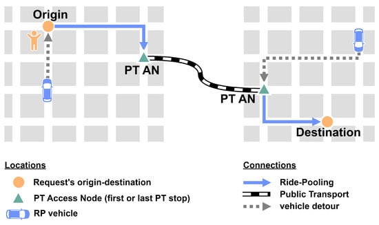 Figure 1. Intermodal 3-leg trip combining ride-pooling (black lines) with public transport (black–white striped line).
Additionally, trip requests have been divided into two types depending on how long in advance they arrive to the system:
- Type HN, for ‘Here and Now’. Requests are placed at that instant and dispatched immediately.
- Type B, for ‘Booking’. Requests are placed well in advance.
A customer’s trip preference has also been taken into account. This may determine the intermodality type in some cases. The following categories have been considered:
- –
- a. Pure-RP. Clients want an RP-exclusive trip. Their trips must be composed of a single leg (RP-only).
- –
- b. Including PT. Clients want a trip with PT included. Their trips must be composed of either one leg (PT-only), two legs (RP + PT or PT + RP) or three legs (RP + PT + RP).
- –
- =. Indifferent. Clients have no preference. Their trips can be made up of one, two or three legs of any type.
3.2. Main Components of the Simulation-Based System
The architecture of the simulation-based system developed in this paper is presented in Figure 2. It consists of two main components: an intermodal dispatcher which, amongst other functions, computes the combined routes, and an intermodal simulator that evaluates the new use case based on simulation. The intermodal dispatcher in turn, is constituted by the Outer Dispatcher, the MaaS Dispatcher (an operational ride-pooling dispatcher developed by the PTV Group and available for internal developments) and the Public Transport Journey Planner (referred to as the PT Journey Planner, which is implemented specifically for this research to cope with the public transport network). The former is the core component that determines the new intermodal routes based on the latter components. The information required to construct the journey legs is obtained through a simulation model with the full definition of the private transport network for the ride-pooling system and the operating timetables for public transport. The intermodal simulator has been developed based on the MaaS Simulator, an exclusive ride-pooling simulator, and adapted to the new intermodal scenario researched here. The same system idea is employed in [12] where the MaaS Simulator is adapted to an electric ride-pooling scenario.
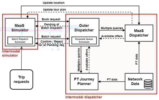
Figure 2.
Architecture of the intermodal system with the batch dispatching approach.
The overall methodology follows an event-scheduling and batch-processing approach that can be described as follows:
Trip requests are defined by the origin–destination locations of the trip and the corresponding booking time requirements. As long as the system evolves, they are queued and grouped in batches by the Requests Queue Scheduler (inside the Outer Dispatcher) with previous requests still pending for a journey dispatch. As it will be shown, a batch of requests may consist of newly issued requests, booked requests whose processing time has come, and requests generated by the system itself, corresponding to the pick-up time of a client in the case of a three-leg journey. The task of the Batch Dispatching Scheduler is to control when the batch dispatching requests should be triggered so that the simulator sends a request to the Outer Dispatcher to compute a journey for all the trip requests in the batch. For the trips with a last leg of RP in their intermodal composition, the adopted approach is to “break” them, leaving the last leg as an RP request to be included on the events list for future processing with a simple anticipatory strategy. Further details are explained in the next Section 3.4. After that, the simulator updates the new tour plans and a new cycle begins. Regularly, vehicle location updates are sent to the MaaS Dispatcher by the MaaS Simulator according to the vehicle tour plans for the upcoming system cycles.
3.3. Intermodal Simulator
The Intermodal Simulator evaluates the use case based on simulation. This component has been developed based on the MaaS Simulator, an exclusive ride-pooling service simulator implemented by PTV Group and available for internal developments, which has been adapted to the characteristics of the intermodal scenario researched here.
This simulator performs an event-scheduling and agent-based simulation with two types of agents: vehicles and customers. The vehicle agent represents a vehicle moving between pick-up and drop-off (PUDO) locations, whereas the customer agent represents a customer booking and performing a trip. In the original implementation of the MaaS Simulator, customers could only experience Pure-RP trips in an immediate dispatch approach (requests were answered immediately with a Pure-RP journey or rejected if no feasibility was found). Thus, it has been extended to the new intermodal scenario so that it could simulate these combined trips that consist of a set of different legs of RP and PT modes. A representation of the resulting customer’s agent states is illustrated in Figure 3 with the areas in black (original) and pink (intermodal extension with the integration of public transport). The blue and green extensions are discussed in the later sections of this document.
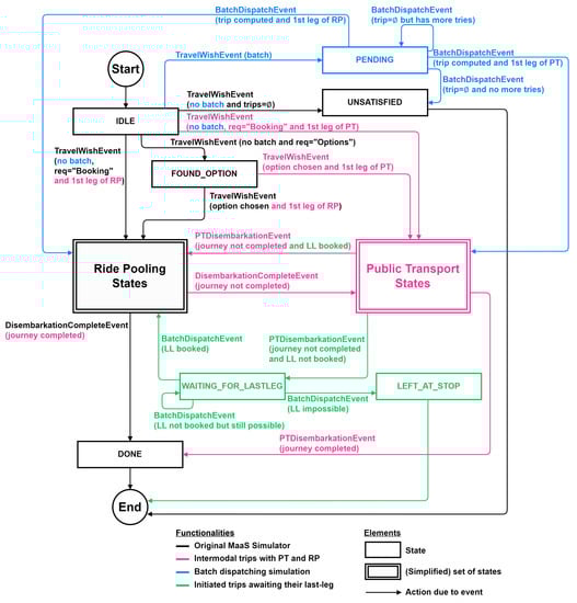
Figure 3.
States in the customer agent’s model and related functionalities.
Batch Dispatching Scheduler
Instead of processing the requests individually, one at a time, as soon as they come, gathering them in small groups (batch) has been shown to be computationally more efficient while giving the opportunity to obtain better quality solutions for the system. On the other hand, the system’s response is delayed by the time required to form a batch. Taking this into account, the batch dispatching approach adopted can be considered a hybrid, since it limits the batch size up to a maximum number of requests or closes the batch after a given time period (i.e., 30 s) is elapsed. The requests in the so-formed batch are passed to the Outer Dispatcher for processing them using a dispatching algorithm (described next in Section 4). In case the dispatching algorithm provides a journey to the request, the simulation of it will proceed. Otherwise, if no feasible journey is found, the request can either be discarded or it can wait until the next batch request is received (details on the actions after a failed dispatch are described in Section 3.4.4). This batch dispatching approach appears reflected in the customer agent states, as shown in blue in Figure 3.
For the configuration of the batch dispatching strategy, a period of 30 s is assumed, which is frequently used in cases of exclusive ride-sharing scenarios, as it appears in [13,14,15]. This value is related to the quality of the service, since on the one hand, it prevents clients from waiting long for a response, and on the other hand, it allows the system to group requests optimising system resources. The batch size, on the other hand, is more related to the performance of our system and the number of requests it can handle in a reasonable amount of time. In this case, a maximum request limit of 30 is set merely to protect the system during peaks of demand.
3.4. Requests Queue Scheduler
This component manages the queue of pending requests in the Outer Dispatcher and decides when a request is dispatched, discarded, left for a future dispatch or requires an additional task.
3.4.1. Requests Scheduling of Trips including a Last Leg of RP
When requests can be resolved with a trip that considers exclusively the public transport or the ride-pooling service on the first leg (with the possibility of transferring later to PT), their assignment can be accurately completed with the current state of the system and can be resolved in a single batch period or postponed to a later one if no feasible solution was found. However, when 2-leg trips (PT + RP) or 3-leg trips (RP + PT + RP) appear, it may be complex to resolve the last leg of RP that will take place ahead in time. Thus, these trips are divided into two separate periods: in a first period, the first part of the trip until the PT leg is dispatched, an estimation of the last leg of RP is made, and a new, artificial RP request is placed ahead in the list of scheduled events, being processed when the time of that last leg of RP approaches. This makes it necessary to consider the so-called requests (referring to last-leg requests) in the list of events. A time-representation example of this approach is shown in Figure 4. Considering a batch period or cycle c, it may contain: (a) requests from the current period (request ), (b) from a previous one if it was not yet dispatched (request ) and (c) with LL-type requests (request from ) which was arranged to be processed with some anticipation so that the client could be picked up readily by a vehicle very close to the time that the public transportation leg is finished.
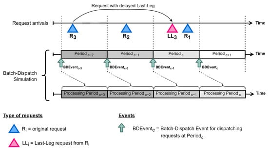
Figure 4.
Time-representation of requests scheduling with delayed last-leg requests.
3.4.2. Relocation of RP Vehicles for Serving LL Requests
As explained previously in Section 3.4.1, requests are placed ahead in the list of events to be processed later. Ideally, an RP vehicle should arrive at the very same moment the client is leaving the PT system to pick him up and take him to his final drop-off point (its original destination). If this does not happen, the client may have to wait for a vehicle, raising the possibility that this LL request cannot be served in time due to the non-availability of an RP vehicle close enough to the final PT-AN where the client must be picked up. In order to prevent as much as possible such undesired situations, a vehicle relocation strategy has been adopted, and within a certain amount of time in advance, an event for triggering the relocation of RP vehicles is placed in the simulator events list. This event will make that an RP vehicle will start moving to the LL pickup location, keeping its capability of performing new PUDOs in between, as long as it arrives at the stop in the desired instant to pick up the client. To determine which vehicle should be relocated, a heuristic is developed taking into account (a) the client’s arrival time at the destination, (b) the travel time to reach the PT-AN (nearest vehicle) and (c) the possible waiting time of the relocated vehicle.
3.4.3. Implications of Delayed Last Legs of RP on Agents’ Behaviour Models
While the vehicle agent behaviour model serves each RP leg as an independent request, the customer agent behaviour model has the possibility of dealing with several legs of RP and PT, consistently with the batch dispatching approach and with the processing of intermodal trips with delayed last legs of RP (PT + RP or RP + PT + RP). The states corresponding to the customer agent behaviour model appear in the previous Figure 3 as well as the related functionalities. The batch dispatching approach requires the requests to be queued as they arrive and leaves them unanswered for some time, entering them in a “PENDING” state, until a batch dispatch serves them. The possibility of delayed last legs forces the customer agent to be able to take into account the eventualities of the transfers between both modes of transport (although possible, the system’s parameters make them very unusual). Thus, it may happen that after ending its PT leg, a client has to wait to be picked up by an RP vehicle and then the customer agent enters into a “WAITING AT STOP FOR LAST LEG” state. The client may stay in this state for an undetermined number of cycles, being almost always picked-up by an RP vehicle. However, if a cycle comes in which the time window requirements of the client can no longer be satisfied, then the client will enter into a “LEFT AT STOP” state, making that no RP vehicle may be considered for performing that infeasible last leg of RP. These two states appear previously highlighted in green in Figure 3.
3.4.4. Prioritised Classification of Requests and Their Dispatching Policies
So far, the request types that have been considered are HN and B (because of promptness) as well as the users’ modal preferences (a, b and =) described in Section 3.1. Considering also the presence of trips with delayed last legs of RP, four sets of requests gathered during a cycle will have to be considered for being resolved by the Outer Dispatcher accordingly to a system of priorities as well as a set of actions on them. The four sets are:
- –
- = set of “Here and Now” requests, i.e., made in the same period. They have the lowest priority and are given two attempts for dispatching.
- –
- = set of Booking requests, i.e., made in advance to the simulation horizon. They have higher priority than HN requests and are given as many dispatch attempts as possible until their time window is overcome.
- –
- = requests that come from trips that have already been dispatched in a previous period as two-leg trips (PT + RP) or as three-leg trips (RP + PT + RP) that in the first cycle estimated their last leg of RP. They are waiting for the system to finally dispatch the last leg. They have the maximum priority and are given as many attempts as possible until their request’s time window can no longer be met. These requests are present in the events list and are included in the current cycle with some anticipation as stated below in Equation (1).
- –
- = set of waiting requests that have entered the system at least in the previous period (batch dispatching period) but have not yet obtained a dispatched trip. These requests were initially included into one of the , or request sets at an earlier cycle, but they have not been yet resolved.
To finally outline the actions adopted by the dispatching policy, there follows a description of (a) the instants where a booking or a last-leg request should be either considered to be dispatched in the current cycle or finally rejected if no feasibility is detected, and (b) the time instant where the vehicle relocations for LL availability should be fired. Notice that these policies actually provide a sharper definition of the previous sets , , and :
- –
- LL requests to dispatch in the current period. Let be the set of requests i, previous to cycle , that result in an LL request and let be the time, counted from cycle c, remaining for the customer of request i to leave the final PT-AN, thus completing the journey until its PT leg. Then, the subset of LL requests, , that will finally be dispatched in the current cycle will be those with an anticipation of at most min, i.e.:
- –
- Booking requests to dispatch in the current period. Let be the time remaining, counted from cycle c, for picking up the customer and let B be the set of Booking requests (negative values for imply that a delay is incurred). Therefore, bookings are taken into account by the scheduler when the time remaining is smaller than a given threshold , which has been estimated to be 30 min. This makes that the set of Booking requests considered for dispatch in the current cycle will be:
- –
- LL requests requiring a vehicle relocation in the current period. An LL request can still wait to trigger a vehicle relocation when it still has some margin until it leaves the PT and has several vehicles that could serve its LL with a small waiting time for the vehicle. Let be the estimated travel time necessary for the RP vehicle j to reach PT-AN of client i (the originator of the LL request). Then, the set of LL requests, , that will need a relocation request to be triggered will be given bywhere the parameters have been adopted as min, min.
- –
- LL requests to reject. LL requests are maintained in the system until its time window is no longer feasible. As they are the longest trips and their time windows are also very long, this will imply that they will be in the system for a very long time. To avoid keeping them in the system for an unnecessary amount of time, it would be convenient to identify the instant at which it is no longer viable to serve them. The set of LL requests to reject in a cycle will be:where is the current time and the latest arrival time at its destination for a request i. is the minimum estimated travel time of the trip that the nearest vehicle would need to go to pick up the client at its current location (the stop) and drop him off at its destination (vehicle’s tour or future detours are not taken into account).
- –
- Booking requests to reject. Given that each B request starts to be considered some time in advance, the total time window that these types of requests are maintained in the system is very large, and the system identifies the time instants when a B request is impossible to be satisfied. Those that will be rejected define the following set:where is the current time, the desired departure time at the origin of the client and is the maximum arrival time at its destination. refers to the minimum estimated travel time of the trip that the nearest vehicle would need to go to pick up the client at its origin and drop him off at its destination (vehicle’s tour or future detours are not taken into account).
A summary of the actions taken on each of the previously defined sets in a given cycle is given in Table 2 below. The table also shows, for each of the sets, the previous priority of their requests (for waiting requests only), their priority and the action to be applied after a failed attempt has occurred for resolving them. The last column specifies the subsets considering the intermodal preference of the requests (a, b and =).
Table 2.
Summary table for the various subsets of requests that are considered by the scheduler and the Outer Dispatcher.
The configuration of the proposed dispatching methodology is related to the quality of service provided by the system. A value of min has been set so that the last-leg dispatchings are delayed in order not to overload the system with too early requests and, on the other hand, the complete tour plan is elaborated around 25 min before leaving the PT system. min enforces Booking requests received in advance, prioritising them above regular requests, and at the same time, it makes it easier for the system to anticipate the vehicle’s availability. The vehicle relocation strategy should be triggered before the last-leg dispatch, so min and of min have been assumed to avoid client requests being left without an available vehicle (e.g., during high-demand peaks). In addition, the system prioritises them over new requests.
3.5. Public Transport Journey Planner
The PT Journey Planner is a schedule-based route planner that computes the PT routes. The procedure is to pre-compute them using rRAPTOR (an extension of RAPTOR in [13]), which computes bi-criteria range queries containing all Pareto sets of journeys for all departures within a time range considering two criteria: the arrival time and the number of transfers. For our intermodal scenario, the maximum number of segments, K, in a PT route will be . i.e., one internal transfer at most in the PT leg. This is because the combination with RP adds more transfers, and this would probably make the intermodal system less appealing and comfortable. This procedure calls RAPTOR multiple times for every origin stop and departure, sorting every departure in decreasing order so that previous calculations can be reused as an upper-bound. Furthermore, for the requirements of this work, the standard version of RAPTOR has been modified in two ways. First, the target pruning is removed so that each RAPTOR execution computes all the PT routes from one origin stop to any other stop (for every single departure). Second, this algorithm permits the last segments to be of walking mode, which is not of interest in the intermodal scenario because the stops are used as the access nodes for transferring between RP and PT. Thus, the K rounds are divided into rounds so it keeps every route and transfer segment individually. Then, only the resulting PT routes ending with a route segment are valid.
When the PT journey planner receives a request for a trip between a given pair of stops, it searches for the earliest one in the pre-computed data which departs right after the specified time. This approach minimises the most time-consuming part of the PT leg calculation because they are already pre-calculated in advance. However, total memory requirements are increased, since all paths comprised within a wide time window must be stored.
4. Outer Dispatcher Methodology and Modelling
The Outer Dispatcher applies a methodology structured in three steps. Initially, there is a heuristic selection of candidate vehicles and stops that can be potentially combined to form intermodal trips. This action is carried out by the so-called ‘Candidates search method’ block, which is described in Section 4.1 below. Next, in a second step, the options for the intermodal combinations are determined as described in Section 4.2. Finally, the decision on the intermodal assignment is determined by means of the so-called “optimal modal trip composition” (OMTC) module that solves an optimisation problem described in Section 4.3, taking into account the stated user preferences and the system of priorities, both ruling the requests in the current cycle.
4.1. Step 1—Candidates Search Method
This method identifies the proper transfer points where customers can switch between modes which are derived from the entire PT network stops. It applies a three-step filtering considering the distances between requests, origin–destination to vehicles and stop locations. First, it restricts the candidates within a search area. Second, it estimates the stations with a proper connection between the origin and destination. Third, it estimates which of these could be served by the vehicles. As a result, non-existent or excessively long travel time connections are filtered out.
This procedure also considers which requests can be scheduled in the form of trips with a last leg of ride-pooling type (PT + RP or RP + PT + RP trips) taking into account the current state of the system.
4.2. Step 2—Computation of Potential Intermodal Trips
This step computes the potential intermodal trips determining the most suitable combination of RP and PT legs using the MaaS Dispatcher and PT Journey Planner. Firstly, the RP vehicles and expected PUDO times are determined, considering the congestion of the RP fleet at that precise time window. Secondly, the departure choices at an origin stop to a set of destination stops are determined, taking into account the concrete departures and arrivals in the timetable. The Outer Dispatcher then aggregates these intermediate results to estimate the feasible assignments for each pending request with its subset of candidate stops. The approach is then as follows:
- –
- For Pure-RP. These trips are resolved with a unique request to MaaS Dispatcher with the original time-windows constraints.
- –
- For Pure-PT. These trips are resolved with a unique request to PT Journey Planner with the original time-windows constraints.
- –
- For RP + PT or RP + PT + RP. First, an initial arrival time at the stop is estimated, considering an estimation of the first RP leg and the congestion of the RP fleet. Afterwards, an appropriate PT departure leaving after the arrival at the stop is computed. This step assumes that the candidate stops that are close to the original destination will be accessed by foot (RP + PT trips). However, for those that are farther away, an appropriate arrival time will be estimated using a last leg of RP. Finally, the first RP leg using the restricted time windows to access the origin stop is determined.
- –
- For PT + RP. Similar to RP + PT + RP case, it assumes that the initial access to the PT stop is performed by foot.
4.2.1. Estimation of a Last Leg of RP
The last legs in RP will take place ahead of the current time instant at which the originating request is being processed, and this makes it challenging to identify the best RP vehicle to serve that LL. Thus, at the request processing time, only a first estimation is made, choosing the RP vehicle with some anticipation to the time instant of the client’s pick up.
The procedure to estimate the request consists of looking for vehicles that, for the time closest to the , are in that area and could serve the required leg, as if no other passengers would be riding on it and taking into account a fare under these conditions. The travel time estimate would then be obtained from the direct journey from the destination stop to its original destination, also with the addition of a waiting time at the stop for the customer if the RP vehicles are far away.
Note that this is an estimation of the travel time and the fare of the last leg. When the definitive vehicle is finally dispatched, these values are updated, as well as when the simulation time progresses and the assigned vehicles make additional detours for other new passengers.
4.2.2. Fare System
The total fare of a combined trip is the sum of each of its legs. In the case of a PT leg, a single ticket fare is used. For the RP leg, a modified version of the fare system proposed by [14] is used, which defines a very simple but adequate method to compute the fare in a ride-pooling service:
where p is the regular taxi fare per km, c is the vehicle’s capacity and is the distance travelled with m passengers. This method assumes that the distance travelled individually is fully paid and the distance shared with other passengers is evenly split considering a small inflation parameter .
The formula has been extended to include a base fare b to reflect how shared services really function in practice (such as Uber and Cabify). However, a minimum fee is not imposed because an RP leg should be substantially shorter in an intermodal scenario compared to a pure ride-pooling one.
Formula (6) for the definition of the fare system is generic, but the specific values of the parameters such as the base fare b and the fare per km p depend on the scenario in which the system is applied. Therefore, the average values of similar companies already operating in the use-case city, in our case the metropolitan area of Barcelona introduced in Section 5, should be assumed. The fare inflation , on the other hand, is related to how much the system increases the fare for shared rides. Low values encourage sharing more of their journey, while high values result in more system profits. For this research, a value of 0.5 will be assumed based on other studies that analyse a fare system for ride-pooling scenarios such as [14,15], which proved that it provided low fares for customers while remaining profitable for the system.
4.3. Step 3—Optimal Modal Trip Composition (OMTC) Module
The OMTC module assigns client requests to RP vehicles included in the current batch by means of an optimisation model that determines the modal composition of the trip requests under the current availability and capacity of RP vehicles as well as the suitable PT-AN locations selected by the previous filtering step described in Section 4.1. Observing Table 2, this module takes into account the type of requests that need to be served at each cycle of the Outer Dispatcher, taking into account their priority level, the user preferences expressed for the request and also whether the requests are new or come from a previous cycle, where they could not be resolved.
The complete formulation of the optimisation model is described below. For the current cycle, it is assumed that there is a set N of requests in the current batch and a set J of vehicles that may satisfy them. The set of requests N will be divided into the subsets that have already been specified previously in Table 2. Set S contains the PT-AN points where clients may be dropped off to continue the trip using public transport. For convenience, vehicle 0 represents the “null-taxi” (not using an RP vehicle) and stop 0 represents the “null-stop” (not using the PT system). This means that a trip with represents the clients not served. Hence, two additional sets are defined for convenience: and .
The model that will be described uses binary variables and , that represent the assignments client-to-vehicle and vehicle-to-stop, respectively. Additionally, variable , defined as the product , represents the assignment of a request to a vehicle visiting a PT-AN. Then, the optimisation model (c1) to (c6) below yields the modal trip composition, as listed in Table 3, depending on the resulting values for variables for a vehicle j and stop k assigned at each request i:
Table 3.
Modal trip composition as provided by the OMTC module.
The model considers the client’s latest arrival time , which corresponds to the request , at the destination. It also presupposes that vehicles are already servicing other passengers, in which case the set of passengers aboard vehicle will be represented by . Each passenger has a latest arrival time and an expected arrival time at his/her drop-off point. Additionally, PT Journey Planner and MaaS Dispatcher assess the following parameters, representing the timings of potential assignments:
- (a)
- is the trip time of request i using PT, i.e., boarding at PT-AN k and travelling to the corresponding alighting PT-AN of request i.
- (b)
- denotes the travel time for vehicle j to pick up the client i and leave it at the PT-AN . If , then is the estimated time used by vehicle to the final destination of client i.
- (c)
- is the additional detour time that passenger will experience if the RP vehicle j he is boarded on picks up request i.
This notation is summarised in Table 4.
Table 4.
Summary of the notation used.
| Minx,y,z,T | ||
| (c1) | ||
| (c1′) | ||
| (c1″) | ||
| (c2) | ||
| (c2′) | ||
| (c2″) | ||
| (c2‴) | ||
| (c3) | ||
| (c4) | ||
| (c5) | ||
| (c6) | ||
| (c6′) | ||
Constraints (c1) to (c1) express the flow balance of binary variables and , whereas constraints (c2) to (c2) are a reformulation of the product in the form of linear constraints. By constraint (c2), if for client i no stop is suitable and no RP vehicle will pick him/her up, then is forced to 0 (request postponed). By constraint (c2), if PT will not be used for serving client i, then the client will not reach any PT station. Because the batch size is assumed to be small, the model assumes that at each cycle, a vehicle picks up at most one client. Forced by constraints (c3) and (c5), variable denotes the expected travel time of client i to his/her destination, which is bounded by its latest possible arrival time and a suitable upper bound . Constraint (c4) ensures that the latest arrival time of passenger p given by will always be observed, taking into consideration the additional detour time for picking up a new client (in (c4), as also in (c5), is simply a big integer and is just the current time instant). Next, constraint (c6) applies to requests i in the class of requests that must be served by RP mandatorily in its only leg (clients with preference a) or in its last leg. If , then the previously mentioned clients will not be served in the current cycle, and if , they will be served by some vehicle. Likewise, constraint (c6) applies for requests of clients with preference b and if no connection will be made, but if , then some connection will be carried out.
The first term in the objective function of the model considers cost parameters , which are the combination of two indices (with weights and ), the user’s trip time and an estimation of the user’s trip fare , which are both normalised by their maximum values and evaluated previously by steps 1 and 2 and the help of the PT Journey Planner and the MaaS Dispatcher. The weights of and will be assumed to look for solutions appealing to the users which could not necessarily be the most convenient economically but take them the fastest to their destination. to are penalty terms to enforce the priorities stated in Table 2.
T1 penalises not serving ‘Here and Now’ requests from the current period. T2 penalises not serving pending ‘Here and Now’. T3 penalises not serving LL and Booking requests from the current period, and finally, T4 penalises not serving LL and Booking pending requests. Then, to ensure the priority of the main sets of requests (HN, B, LL and W), penalty coefficients , , and should verify , which is guaranteed if they are adopted as follows:
5. Computational Experiments
5.1. Case Study: City of Barcelona
The intermodal simulation model of this paper has been tested on the inner region of the metropolitan area of Barcelona, in Spain, as shown in Figure 5, comprising several municipalities, the most important of them being the city of Barcelona as a strong attractor of trips and activities from the surrounding cities. Those included in the Test Area of this paper (referred to simply as TA in the following) have been Barcelona itself, L’Hospitalet del Llobregat (southwest), Sant Adrià del Besòs and a portion of Badalona and Santa Coloma de Gramanet. In all, the TA has an extension of nearly a 20 × 15 km area of a very large urban density.
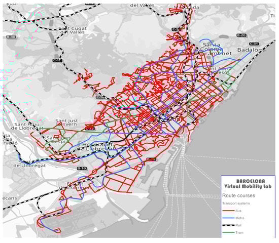
Figure 5.
The test area showing the various types of public transportation lines.
The PT network under consideration in the TA has been made up of PT facilities in the Integrated System for Metropolitan Mobility of Barcelona (SIMMB), i.e., the bus, metro and tram lines, and the rapid transit systems operated by the Generalitat de Catalunya. Additionally to the SIMMB, the Spanish railways (RENFE) have also been included. All of them make up a large PT network with about 3000 stops, nearly 300 distinct lines and more than 6000 services during the operational horizon assumed in the tests (from 9 to 13). Moreover, the private traffic network is constituted of 114,000 links and 87,300 nodes. This contrasts significantly from other studies in the literature, which employ either a small test area or with a very tiny portion of the entire PT network.
As a reference, Table 5 below shows the average trip travel times for each of the transportation options employed in the test area. This information has been obtained using the Virtual Mobility Lab network model developed in [16], being refined and adapted by the authors during the development of this intermodal simulation system.
Table 5.
Trip travel times (min) in the SIMMB. InterM = between different municipalities, IntraM = internal to a municipality.
Like many other Spanish cities such as Madrid ([17,18]), Seville ([19]) and similar large metropolitan areas in the world, Barcelona’s metropolitan area has an extensive public transit network on which many people rely on a daily basis, a solid high-capacity private transit network, and the emergence of innovative shared mobility services such as ride-pooling (Uber, Cabify, etc.) and motorbike-sharing (eCooltra, SEAT MÓ, etc.), which have steadily gained popularity since their disruption ([20,21]). A characteristic shared in common by all large metropolitan areas is the one depicted in Figure 6 for the city of Barcelona, where the majority of morning commutes originate from various locations throughout the area but are mainly headed to the city centre, which houses the majority of businesses and entertainment. Additionally, as evidenced by studies such as [22], movements inside the city of Barcelona are frequently undertaken using the public transit network. Its usage may, however, diminish when the origin or destination is on the outskirts due to a more limited variety of options, which forces them to switch to private alternatives. As a result, the entire metropolitan region is an ideal scenario for testing the proposed intermodal approach to connect users in places where this transit offer is inefficient, which will use the ride-pooling service as a feeder for the public transport, reducing customers’ dependency on private mobility.
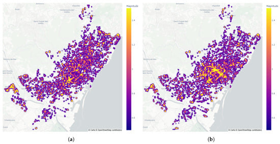
Figure 6.
Demand movements in Barcelona from 9 a.m. to 13 p.m. (a) Origins. (b) Destinations.
5.2. Test Scenarios
To illustrate the system’s viability, three tests have been run on the previously described area, whose characteristics are shown in Table 6 below. All the tests assume that a majority of the requests are of the ‘HN’ type (80%), and only 20% of bookings take place. The first test assumes only requests demanding service exclusively by RP, and it has been included for reference. In contrast, tests 2 or 3 have little or no trips demanding exclusively RP (although the system might assign by itself this modal option in some cases). In all three tests, a number of 10,031 trip requests have been generated by the system during a period of time of 4 h (from 9 to 13) to account for the beginning and end of trips, which is equivalent to an approximate fraction of 20 % of the demand in public transport between the satellite municipalities and the central city.
Table 6.
Experimental instances summary with the type of requests and intermodal preference proportions.
The simulations have used a fleet of 400 RP vehicles with a capacity of four passengers during that period, which is a capacity frequently used in ride-pooling scenarios such as [23]. The ride-pooling service’s fare is based on the reported fare from equivalent enterprises already presently operating in Barcelona, set to a 0.5 € base fare, a 1.28 € fare per km and a 0.5 fare inflation (obtained from the average fare costs of Uber and Cabify in Barcelona (Spain) on 15 August 2022, when these experiments were planned. Source: https://www.uber.com/global/en/price-estimate/ (accessed on 15 August 2022) and https://cabify.com/es/barcelona/lite/tarifas (accessed on 15 August 2022)). A public transportation fare in the SIMMB of 1.14 € (obtained from the fare of one ticket from a 10-ticket travel card in Barcelona. Source: https://www.tmb.cat/es/tarifas-metro-bus-barcelona/sencillos-e-integrados/ (accessed on 15 August 2022)) has been assumed.
In order to evaluate the performance indices of the system, a set of experiments have been carried out through which it has been possible to evaluate, on the one hand, the effect of the batch dispatching parameters and, on the other, it has been verified that the established anticipation times were appropriate. The parameters associated with batch dispatching are in turn related to the time to be able to respond to a set of requests, which can be critical in case of potential saturation. A batch dispatch period of 30 s could be assumed as used by many ride-pooling studies. For the batch size, however, a sensitivity analysis is carried out to establish a preliminary value. Table 7 depicts some results to illustrate its effect on the system performance.
Table 7.
Sensibility analysis on batch size. Average CPU running times distribution per batch.
Experiments have been carried out on an Intel Core i7-10700 Machine (8-core, 16 threads, 2.90 GHz up to 4.80 GHz Turbo), with 32 GB of DDR4-2666 RAM. Column #Req shows the average number of requests (including LL requests) taken into account in each batch. The average simulation time gap between batch dispatchings appears in column Freq. Column Total batch time is the average CPU time taken to perform the dispatching of a batch and divides approximately between the three steps of the dispatching method reported in the adjacent columns. The optimisation model in Step 3 is solved using Gurobi with a limitation in time of s each run, which on average provides solutions with an approximate relative MIP optimality gap of . Column Total time reports the total running time taken for each of the experiments. As clearly seen, low values make it difficult for the system to dispatch promptly, and high values, as predicted, saturate the system with lots of requests, making it impossible to respond to all of them in an acceptable short time. Moreover, the optimisation model (Step 3) takes 3× longer to solve a request, indicating that the model size may be too large.
As a result, a batch size of 10 requests will be set for the experiments presented in this paper to obtain near to optimal performance of the system during high-demand peaks.
5.3. Results
As Table 8 shows, the option for intermodal trips benefits the RP system since the number of not served requests (Not Served) reduces from ∼67% in test 1 to ∼15% and ∼11% in tests 2 and 3, respectively. Another aspect, as shown in column Left at stop, is the number of clients that have not completed a trip with a last leg of ride pooling, which may be of the PT+RP or three-leg trips type that are dispatched; none is left at a stop.
Table 8.
Summary of served demand and intermodal options used.
Table 9, Table 10 and Table 11 provide average travel trip times, distances and fares. In all tables, column “RP trips” refers to trips with RP only, “PT trips” refers to trips with PT only, “RP + PT trips” refers to trips with two legs starting by RP and later transferring to PT, “PT + RP trips” refers to trips with two legs starting by PT and later transferring to RP, and those with three legs appear under “3-Leg trips”. In the rows, “Direct” refers to the individual trip with exclusive RP (used as a reference for comparison with the one dispatched), “Expected” refers to the trip initially reported by the system (the dispatched one), and “Actual” refers to the experienced one at the end of the simulation after all future detours. From these intermodality options, a two-leg trip including public transport shows the best indicators. Since RP-only trips face directly urban congestion in the centre, they have a larger travel time (Total) and higher costs for the user, (Fare). In contrast with this, any other type of trip presents a fare remarkably cheaper than any other with a reduced travel time precisely because they skip the congestion in the centre. When compared to an RP-only trip, a trip with three legs, although with larger travel time, covers a much larger distance for a lower cost. In addition, any two-leg trips can reduce a longer trip by half the cost. In all cases, the waiting time in transfers (wait) and the walking time to the user’s destination (walk) in two- or three-leg trips appear reasonably small, incentivising commuters in surrounding cities to possibly become new users of the RP system.
Table 9.
Summary of mean travel times for RP, PT and RP + PT trips.
Table 10.
Summary of mean travel times for PT + RP and 3-leg trips.
Table 11.
Summary of mean experienced distances and user fares (no sharing) for RP, PT, RP + PT, PT + RP and 3-leg trips.
Table 12 and Table 13 show how fast the system responds to users. The first one reports the average delay times for all requests, and the second reports the average delay times for the subset of trips dispatched with a last leg (PT+RP and 3-leg trips) distinguished if a vehicle reservation has been made. The system manages to provide a tour plan on average in 6 s, with a last leg eventually dispatched between 11 and 23 min later. On the other hand, if the request cannot be served, the system rejects them on average between 12 s (Here and Now requests) to 1.7 min (Booking requests). This difference comes from the fact that an HN request is performed immediately and there is very little margin to serve it. On the other hand, B requests, even if placed 30 min in advance, are considered unserviceable if they remain in the system for an extended length of time.
Table 12.
Summary of time delays in the system decisions.
Table 13.
Summary of time delays in the system decisions for trips with a last leg (PT + RP or 3-leg trips).
In all cases, the system is economically viable, as shown in Table 14, which collects the results for the “full-regime” central period of 2 h (10 h to 12 h) of the ride-pooling service. This estimate assumes a driver’s hourly wage of 8.13 €/h (a 1300 € monthly salary has been assumed, which is obtained from the average gross salary reported by Uber and Cabify drivers in Barcelona (Spain). Source: https://es.indeed.com/career/salaries (accessed on 15 August 2022)), a vehicle fuel consumption of 5.5 L/100 km (obtained from the average consumption of the different model cars reported by Cabify in Spain. Consumptions according to standard WLTP. Source: https://www.km77.com/ (accessed on 15 August 2022)) and a fuel cost of 1.78 €/L (the average fuel cost in Barcelona (Spain) on 15 August 2022 is assumed when these experiments were planned.). The total fare paid by users for their RP legs appears in column Revenues. Of course, the big difference in the profit is because the level of demand is the same as in Experiment 1, but all the users have a preference for RP, which is the most expensive option. It is also shown that the fuel consumption by the fleet of RP vehicles (RP-Fuel) is practically the same in all three experiments. This shows the environmental and social benefits of the intermodal system, taking into account that the fraction of served clients increases with the presence of PT.
Table 14.
Profit analysis for 10–12 h, central period (without warm-up and cool-down periods).
Finally, Table 15 shows the computational performance of the simulation system, which uses the same column definition as Table 7. According to these reports, the system appears to receive a significant number of requests in a short period of time, and as a result, it closes the batches when the maximum size is reached (10 requests). This reduces the time gap between batches to between 6 and 11 s rather than the 30 s initially configured. This is not a problem because the system can respond to them in less than 5 s before the next batch is generated.
Table 15.
Performance statistics. Average CPU running times distribution per batch.
6. Conclusions
This article has described an agent-based simulation model to study the integration of public transport services and a ride-pooling system, this initiative being one of the International Union of Public Transport (UITP) proposals for complementing public transport services in urban areas with less coverage to take advantage of being close to neighbour urban centres with a higher density of PT services.
The simulation model assumes that users may book trips or make requests for prompt service to a centralised system of dispatching, which is able to resolve the requests by assigning them a ride-pooling vehicle that will drive them directly to their destination or to a suitable access point of the PT network, thus starting a second leg in PT. In this case, it will lead the client to a station or stop already close to its destination or where another RP vehicle will complete a third leg ending at the destination. Additionally, if the client has good public transit connectivity from the beginning of his journey, the system may decide to serve him directly via public transportation, which will lead the client to a station close to his destination or where an RP vehicle will complete a second leg ending at the destination.
The simulation system is composed of an adaptation of the MaaS Simulator with its own MaaS Dispatcher (originally a ride-pooling simulator), which is a public transport route planner based on the rRAPTOR model ([13]), and the Outer Dispatcher, which by means of a system’s batch scheduler groups periodically the requests and determines the intermodal composition of the trips and the number of legs for the requests of a batch by means of an optimisation model, whose parameters are heuristically determined by two previous pre-processing steps. The system has been tested on the inner region of Barcelona’s densely populated metropolitan area. The simulations show that travel times and user fares are competitive, especially for the two- and three-leg trips and that the system is appealing as it may not only act as a feeder for the central PT system but also for the RP system, since commuters in the surrounding areas may become its clients.
The simulation experiments conducted in this paper have been made by setting the main system parameters and policies either using the most common values accepted in the available literature for systems with some similarities or by reasonable judgement based on the characteristics of the testing scenario.
Author Contributions
Conceptualization, methodology, E.L., E.C., J.B. and K.N.; writing—original draft preparation and formal analysis, E.L., E.C. and J.B.; software, data curation and visualization, E.L.; project administration, supervision and validation, E.C., J.B. and K.N. All authors have read and agreed to the published version of the manuscript.
Funding
This research was funded by an Industrial PhD by the Generalitat de Catalunya and the company PTV-AG under Grant DI-071 2019; and a research project of the Spanish R+D Programs under Grant PID2020-112967GB-C31.
Institutional Review Board Statement
Not applicable.
Informed Consent Statement
Not applicable.
Data Availability Statement
Not applicable.
Acknowledgments
Special thanks to Dorothea Wagner and Jonas Sauer, from the Institute of Theoretical Informatics at Karlsruhe Institute of Technology (KIT). Many thanks also to inLabFIB-UPC, a research laboratory of the Barcelona School of Informatics (FIB) at the Polytechnic University of Catalonia (UPC) for allowing us to use one of their machines for the experiments.
Conflicts of Interest
The authors declare no conflict of interest.
Abbreviations
The following abbreviations are used in this manuscript:
| RP | Ride-Pooling |
| PT | Public Transport |
| AN | Access Node |
| HN | Here and Now Request |
| B | Booking Request |
| LL | Last-Leg Request |
| ITF | International Transport Forum |
| UITP | International Union of Public Transport |
References
- UITP Technical Report. Mobility as a Service. Technical Report, 2019. Available online: https://cms.uitp.org/wp/wp-content/uploads/2020/07/Report_MaaS_final.pdf (accessed on 13 March 2023).
- UITP Policy Brief. Autonomous Vehicles: A Potential Game Changer for Urban Mobility. Technical Report, 2017. Available online: https://cms.uitp.org/wp/wp-content/uploads/2020/06/Policy-Brief-Autonomous-Vehicles_2.4_LQ.pdf (accessed on 13 March 2023).
- ITF. Shared Mobility Simulations for Lyon; ITF Policy Papers; OECD Publishing: Paris, France, 2020. [CrossRef]
- Hickman, M.; Blume, K. Modeling Cost and Passenger Level of Service for Integrated Transit Service. In Computer-Aided Scheduling of Public Transport; Voß, S., Daduna, J.R., Eds.; Springer: Berlin/Heidelberg, Germany, 2001; pp. 233–251. [Google Scholar] [CrossRef]
- Liang, X.; de Almeida Correia, G.H.; van Arem, B. Optimizing the service area and trip selection of an electric automated taxi system used for the last mile of train trips. Transp. Res. Part Logist. Transp. Rev. 2016, 93, 115–129. [Google Scholar] [CrossRef]
- Stiglic, M.; Agatz, N.; Savelsbergh, M.; Gradisar, M. Enhancing urban mobility: Integrating ride-sharing and public transit. Comput. Oper. Res. 2018, 90, 12–21. [Google Scholar] [CrossRef]
- Pinto, H.K.; Hyland, M.F.; Mahmassani, H.S.; Ömer Verbas, I. Joint design of multimodal transit networks and shared autonomous mobility fleets. Transp. Res. Part Emerg. Technol. 2020, 113, 2–20. [Google Scholar] [CrossRef]
- Liu, Y.; Ouyang, Y. Mobility service design via joint optimization of transit networks and demand-responsive services. Transp. Res. Part Methodol. 2021, 151, 22–41. [Google Scholar] [CrossRef]
- Lorente, E.; Barceló, J.; Codina, E.; Noekel, K. An Agent-based Simulation Model for Intermodal Assignment of Public Transport and Ride Pooling Services. Presented at the 2021 International Symposium on Transportation Data and Modelling (ISTDM 2021), Virtual due to COVID-19, Virtual, 21–24 June 2021. [Google Scholar]
- Lorente, E.; Barceló, J.; Codina, E.; Noekel, K. An Intermodal Dispatcher for the Assignment of Public Transport and Ride Pooling Services. Transp. Res. Procedia 2022, 62, 450–458. [Google Scholar] [CrossRef]
- Lorente, E.; Barceló, J.; Codina, E.; Noekel, K. A Simulation System for Intermodal Assignment of Public Transport and Ride Pooling Services. Presented at the 8th International Workshop on Freight Transportation and Logistics(ODYSSEUS 2021), Tangier, Morocco, 4–10 May 2022. [Google Scholar]
- Jamshidi, H. Dynamic Planning for Recharging Shared Electric Taxies. Ph.D. Thesis, Delft University of Technology, Delft, The Netherlands, 2019. [Google Scholar]
- Delling, D.; Pajor, T.; Werneck, R. Round-Based Public Transit Routing. Transp. Sci. 2015, 49, 591–604. [Google Scholar] [CrossRef]
- Ma, S.; Zheng, Y.; Wolfson, O. T-share: A large-scale dynamic taxi ridesharing service. In Proceedings of the International Conference on Data Engineering, Brisbane, QLD, Australia, 8–12 April 2013; pp. 410–421. [Google Scholar]
- Asghari, M.; Deng, D.; Shahabi, C.; Demiryurek, U.; Li, Y. Price-Aware Real-Time Ride-Sharing at Scale: An Auction-Based Approach. In Proceedings of the 24th ACM SIGSPATIAL International Conference on Advances in Geographic Information Systems (SIGSPACIAL ’16), Burlingame, CA, USA, 31 October–3 November 2016; Association for Computing Machinery: New York, NY, USA, 2016. [Google Scholar] [CrossRef]
- Montero, L.; Linares, P.; Salmerón, J.; Recio, G.; Lorente, E.; José Vázquez, J. Barcelona Virtual Mobility Lab: The multimodal transport simulation testbed for emerging mobility concepts evaluation. In Proceedings of the Tenth International Conference on Adaptive and Self-Adaptive Systems and Applications, ADAPTIVE 2018, Barcelona, Spain, 18–22 February 2018. [Google Scholar]
- Matas, A. Demand and Revenue Implications of an Integrated Public Transport Policy: The Case of Madrid. Transp. Rev. 2004, 24, 195–217. [Google Scholar] [CrossRef]
- Arias-Molinares, D.; Carlos García-Palomares, J. Shared mobility development as key for prompting mobility as a service (MaaS) in urban areas: The case of Madrid. Case Stud. Transp. Policy 2020, 8, 846–859. [Google Scholar] [CrossRef]
- Christodoulou, A.; Christidis, P. Evaluating congestion in urban areas: The case of Seville. Res. Transp. Bus. Manag. 2021, 39, 100577. [Google Scholar] [CrossRef]
- Hasselwander, M.; Bigotte, J.F.; Fonseca, M. Understanding platform internationalisation to predict the diffusion of new mobility services. Res. Transp. Bus. Manag. 2022, 43, 100765. [Google Scholar] [CrossRef]
- Gilibert, M.; Weymar, A. Case study on the use and adaptation of SEAT MÓ motorbike sharing service in Barcelona in COVID-19 pandemic year. Case Stud. Transp. Policy 2022, 10, 591–597. [Google Scholar] [CrossRef] [PubMed]
- Gilibert Junyent, M.; Ribas Vila, I.; Rodríguez Donaire, S. Analysis of mobility patterns and intended use of shared mobility services in the Barcelona region. In Proceedings of the ETC Conference 2017, Barcelona, Spain, 21–24 August 2017; pp. 1–20. [Google Scholar]
- Alonso-Mora, J.; Samaranayake, S.; Wallar, A.; Frazzoli, E.; Rus, D. On-demand high-capacity ride-sharing via dynamic trip-vehicle assignment. Proc. Natl. Acad. Sci. USA 2017, 114, 462–467. [Google Scholar] [CrossRef] [PubMed]
Disclaimer/Publisher’s Note: The statements, opinions and data contained in all publications are solely those of the individual author(s) and contributor(s) and not of MDPI and/or the editor(s). MDPI and/or the editor(s) disclaim responsibility for any injury to people or property resulting from any ideas, methods, instructions or products referred to in the content. |
© 2023 by the authors. Licensee MDPI, Basel, Switzerland. This article is an open access article distributed under the terms and conditions of the Creative Commons Attribution (CC BY) license (https://creativecommons.org/licenses/by/4.0/).