Classification of Interpretation Differences in String Quartets Based on the Origin of Performers

Abstract

Music Information Retrieval aims at extracting relevant features from music material, while Music Performance Analysis uses these features to perform semi-automated music analysis. Examples of interdisciplinary cooperation are, for example, various classification tasks—from recognizing specific performances, musical structures, and composers to identifying music genres. However, some classification problems have not been addressed yet. In this paper, we focus on classifying string quartet music interpretations based on the origin of performers. Our dataset consists of string quartets from composers A. Dvořák, L. Janáček, and B. Smetana. After transferring timing information from reference recordings to all target recordings, we apply feature selection methods to rank the significance of features. As the main contribution, we show that there are indeed origin-based tempo differences, distinguishable by measure durations, by which performances may be identified. Furthermore, we train a machine learning classifier to predict the performers’ origin. We evaluate three different experimental scenarios and achieve higher classification accuracy compared to the baseline using synchronized measure positions.

1. Introduction

Music Information Retrieval (MIR) deals with extracting, processing, and organizing meaningful features from music material [1]. From the analysis of audio signals to symbolic representations and musical blueprints (score), MIR focuses on many challenging tasks such as content-based search, music tagging, automatic transcription, feature detection, music recommendation, and much more [2]. MIR methods significantly impact the Music Performance Analysis (MPA) field [3], providing more accurate detectors and possibilities for automated music analysis. In the case of classical music, a performance affects how listeners perceive a piece of music. Each interpretation may be special thanks to, for example, modifying information from the score and converting various musical ideas into musical renditions [1]. The communication between members of ensembles also shapes a performance [4,5,6]. Classification tasks, such as the classification of music genres [7,8], mood [9], music structures [10], or composers [11,12], are examples of interdisciplinary approaches—a combination of MIR techniques with MPA, musicology, and music analysis.

Music-related classification problems are common [8,13], but only the minimum deals with the classification of origin-based or music school-related differences of interpretations. In this paper, we combine MIR techniques with MPA goals. We focus on identifying the differences between interpretations of the same musical composition. In other words, we aim to create a classifier that could differentiate music performances based on the origin of a given composer. If it is possible to train a classifier, we can conclude that there are noticeable differences. To our best knowledge, there is only one study [14] with a similar goal using machine learning besides studies with a phylogenetic approach [10] or comparative music analysis [15,16,17]. However, many studies combine MIR and MPA disciplines and focus on expressive performances [18,19]. Machine learning models have been researched in the MPA community to, for example, model nuances of dynamics and timing of expressive performances using inter-onset-intervals with Hidden Markov Models [20] and linear regression [21], or to perform score following tasks [22]. Many other approaches to computational modeling of expressive performance also include neural networks [21,23,24].

We focus on string quartet music from Czech composers Antonín Dvořák, Leoš Janáček, and Bedřich Smetana. First, we collect a large dataset (compared to the average size of MPA datasets, see [3]) and label each recording to create two classes: Czech and non-Czech interpretations. The underlying hypothesis is that the Czech performers may play the piece differently, for example, considering the same cultural background and tradition shared with the composers of the analyzed music. We can address this problem quantitatively thanks to the increasing number of available recordings and the accuracy of synchronization methods [25,26]. We extract relevant timing-related features from all interpretations that may cover information about the expressiveness of a given performance and construct feature matrices to train and test a machine learning classifier. 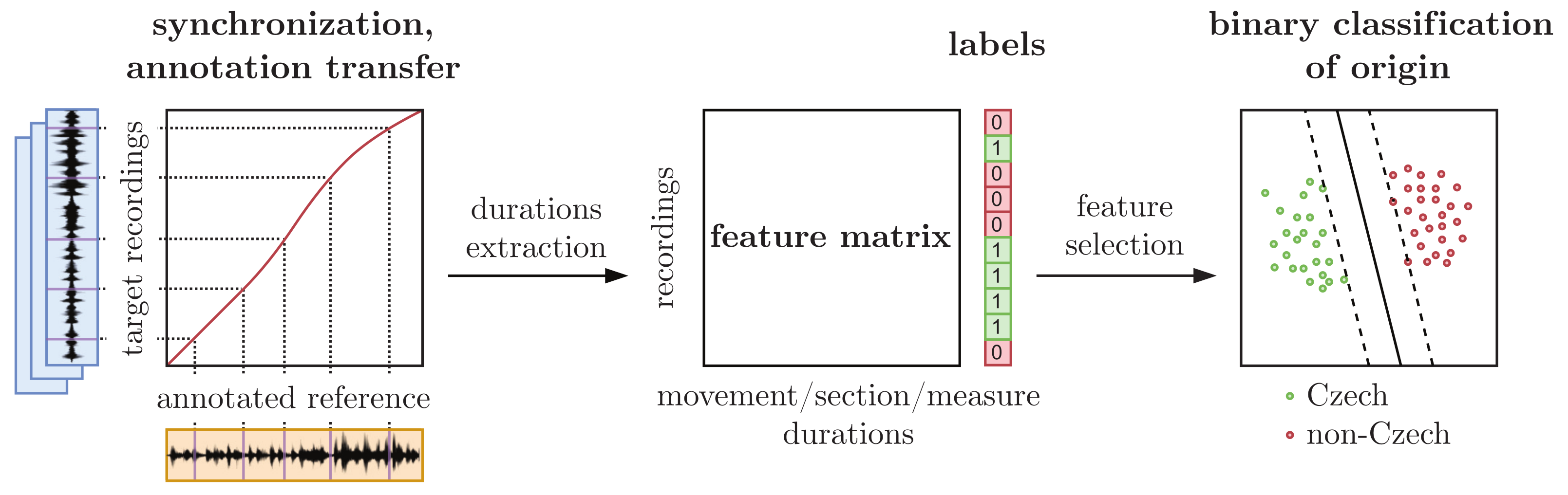Figure 1 shows the overview of our classification approach.

As this paper’s main contribution, we show a general trend in the rhythmic conception (duratas) of given string quartets based on the proposed binary classes. Although various music schools, cultures, and traditions influence musicians, we can train a classifier to identify Czech and non-Czech interpretations of given string quartets with relatively high accuracy in most cases. To better understand the features and classification results (and why it is possible to train such a classifier), we split our experiments into three scenarios, each applying a different time resolution of features. Unlike the approach in the Ref. [14], we use various string quartets, more recordings, and extract features based on a semi-automated approach instead of relying on automated systems with a possibility of significant misdetection. Furthermore, we support our feature selection with MPA principles (see Section 3.1) to focus only on timing parameters that may show the expressiveness of music performances (third scenario). We can achieve high classification accuracy if the selected features, derived from ground-truth (GT) data and a synchronization strategy, capture local tempo deviations. We understand the controversial nature of defining the “origin” of musicians and splitting our dataset into two binary classes; however, we want to show that the interpretation differences may be significant when using a machine learning method, even though they would not be qualitatively noticeable by music experts. We do not claim that a difference in interpretation has any quality to it—we only show that there is a difference. To provide additional data, we share a GitHub repository (github.com/xistva02/Classification-of-interpretation-differences, accessed on 10 March 2023).

The rest of the paper is organized as follows. Section 2 introduces the string quartet dataset, annotation, labeling process, and audio-to-audio synchronization and compares automated and semi-automated approaches for measure detection. Section 3 describes a feature selection, visualization method, dimensionality reduction, and design of experiments. The results are reported in Section 4, followed by a discussion in Section 5 and conclusions with prospects for future work in Section 6.

2. Methods

This section introduces our string quartet dataset, annotation process, and audio-to-audio synchronization strategy to obtain transferred measure positions. We show the validity of synchronization accuracy by comparing the automated downbeat tracking systems with the semi-automated synchronization procedure.

2.1. Dataset

We collected string quartets of Antonín Dvořák, Leoš Janáček, and Bedřich Smetana from various sources, such as Naxos Music Library, Czech Museum of Music, and Masaryk University, Faculty of Arts. Each composition is divided into four movements—in the following text, each movement is regarded as a separate recording. The composers, compositions, and movements (roman numerals) are divided as follows.

• Antonín Dvořák:

  -

  String Quartet No. 12 in F major, Op. 96

  I.

  Allegro ma non troppo

  II.

  Lento

  III.

  Molto vivace

  IV.

  Vivace ma non troppo

  -

  String Quartet No. 13 in G major, Op. 106

  I.

  Allegro moderato

  II.

  Adagio ma non troppo

  III.

  Molto vivace

  IV.

  Andante sostenuto

  -

  String Quartet No. 14 in A♭ major, Op. 105

  I.

  Adagio ma non troppo

  II.

  Molto vivace

  III.

  Lento e molto cantabile

  IV.

  Allegro non tanto

• Leoš Janáček:

  -

  String Quartet No. 1, “Kreutzer Sonata”, JW 7/8

  I.

  Adagio con moto

  II.

  Con moto

  III.

  Con moto – Vivace – Andante – Tempo I

  IV.

  Con moto

  -

  String Quartet No. 2, “Intimate Letters”, JW 7/13

  I.

  Andante

  II.

  Adagio

  III.

  Moderato

  IV.

  Allegro

• Bedřich Smetana:

  -

  String Quartet No. 1 in E minor, “From My Life”, JB 1:105

  I.

  Allegro vivo appassionato

  II.

  Allegro moderato à la Polka

  III.

  Largo sostenuto

  IV.

  Vivace

  -

  String Quartet No. 2 in D minor, JB 1:124

  I.

  Allegro

  II.

  Allegro moderato

  III.

  Allegro non più moderato, ma agitato e con fuoco

  IV.

  Presto

For more details about compositions, we refer to the International Music Score Library Project (IMSLP) (https://imslp.org/, accessed on 10 March 2023). Most versions are studio recordings, but we also keep the live versions.

Table 1. The original dataset of string quartets from Czech composers; composer (csr), composition (com), the number of different interpretations (recs), class 1 (Czech interpretation), class 0 (non-Czech interpretation), and total duration (dur) of all recordings in hh:mm:ss or dd:hh:mm:ss format.

csr	Dvořák			Janáček		Smetana
com	No. 12	No. 13	No. 14	No. 1 *	No. 2	No. 1	No. 2	$\mathsf{\Sigma }$
recs	304	100	92	264	280	171	104	1315
class 1	72	40	40	88	80	75	84	479
class 0	232	60	52	176	200	96	20	836
dur	32:34:28	15:58:55	12:22:27	19:52:32	30:08:06	20:36:51	8:01:24	05:19:34:43

* in this case, the number of recordings varies within movements.

shows the composers, musical compositions, the number of recordings, binary labels (classes) of the performer’s origin (1 refers to the Czech class and 0 to the non-Czech class), and the total duration of all interpretations of the given composition combined. Our dataset consists of 1315 string quartet recordings with a total duration of roughly six days. We focused on the well-known string quartets of Czech composers, increasing the probability of gathering enough data for the proposed analysis.

We understand this labeling is problematic (performers may study abroad and be inspired by many composers, teachers, musicians, and interpretations). However, Czech musicians may play the string quartets of Czech composers differently, inheriting a specific style or carrying on the music tradition that led to the compositions in the first place. Such labeling could be later changed (such as Europe/rest of the world or Central Europe/Western Europe) with different aims of the analysis. As we show in this study, specific details in the tempo of measures may differentiate performers, perhaps even without their prior intention.

Based on the open-source policy, we would like to contribute with string quartet data to the performance datasets (see [3,27]). However, the vast majority of recordings are not under a CC license. Therefore, we share at least measure information (annotations) of each interpretation and composition in the GitHub repository.

2.2. Annotation

To characterize or evaluate differences in interpretations, we want to obtain or extract reliable timing information from each recording (see Section 3.1). First, we used automated methods with little success (see Section 2.4). We manually annotated one interpretation (chosen as a reference recording) per composition to obtain GT data and acquire annotations for all other interpretations based on the audio-to-audio synchronization strategy [25].

We considered the sequence of beats or measures as our timing parameter. Both can describe a given piece’s local and global tempo and can be connected to the underlying score material. However, we chose measures to easily segment sections based on the score and reduce the time needed to annotate each reference recording. Time positions of measures may provide sufficient resolution and valuable information for further evaluation [28]. If the goal of analysis or required time resolution changes, one can annotate and synchronize, for example, beats instead (see Section 2.3).

We annotated GT measure positions (obtaining reference measure positions) for each reference recording based on a corresponding score. Furthermore, we annotated sections—meaningful segments of each movement usually marked by numbers or letters.

Table 2. The number of sections and annotated measures for all recordings of our dataset; composers, compositions, and movements; x means that data are not available—either we did not obtain this information from a score or the chosen reference recording was different from the available score, so we excluded given recordings from the analysis.

Composer	Composition	mov	No.  of Sections	No.  of Measures
Dvořák	No. 12	mov1	19	239
		mov2	9	97
		mov3	13	244
		mov4	16	382
	No. 13	mov1	14	393
		mov2	10	202
		mov3	13	510
		mov4	12	563
	No. 14	mov1	11	204
		mov2	x	x
		mov3	7	102
		mov4	15	534
Janáček	No. 1	mov1	8	164
		mov2	14	236
		mov3	9	103
		mov4	16	189
	No. 2	mov1	17	314
		mov2	17	218
		mov3	15	216
		mov4	24	356
Smetana	No. 1	mov1	12	262
		mov2	12	250
		mov3	10	97
		mov4	18	285
	No. 2	mov1	x	140
		mov2	x	187
		mov3	x	76
		mov4	x	x

shows the number of sections and measures for all compositions and movements. We did not annotate sections of Smetana’s String Quartet No. 2 as they were not included in the score.

2.3. Synchronization

To obtain measure positions for each interpretation, we resample all recordings to 22,050 Hz and compute the time alignment of the reference and all target recordings following the sync-toolbox pipeline in [25]. First, a variant of chroma vectors, also known as Chroma Energy Normalized Statistics (CENS) features [29], is computed. The tuning is estimated to shift CENS accordingly, and the Memory-restricted Multiscale DTW algorithm (MrMsDTW) [30] is applied to find the optimal alignment between both recordings (chroma representations). Measure positions are then transferred from the reference to each target recording based on the warping path and final interpolation. Following this strategy, one can obtain any time-related annotation (onsets, beats, measures, regions) if both reference and target recordings follow the same harmonic and melodic structure and at least one set of GT data is available.

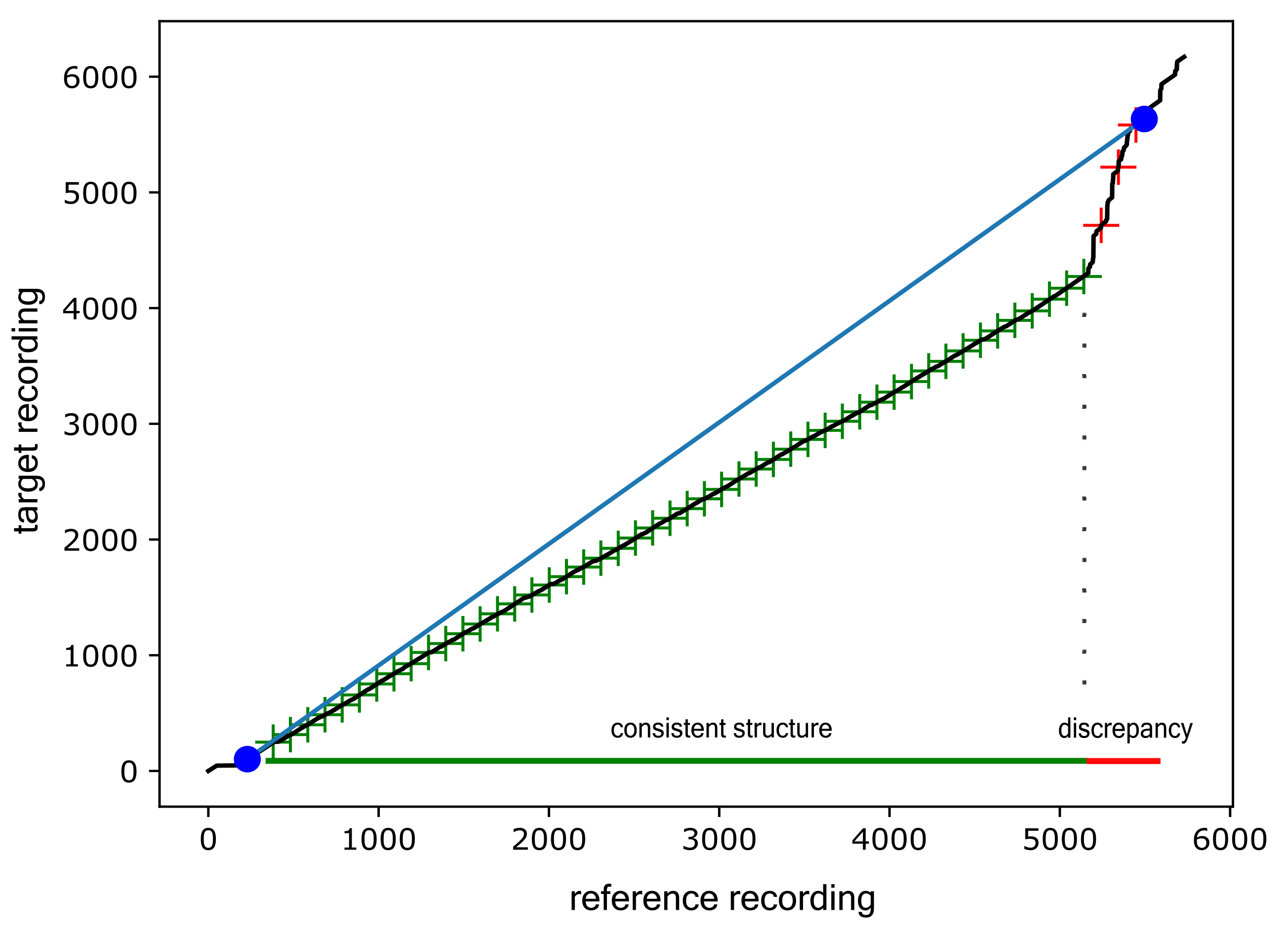
In the case of string quartets, there may be problems with repetitions and, for example, codas. As a pre-processing step, we check the structure differences first. We compute anchor points (the first 10% and the last 90% of the duration of a given recording), test points projected on the warping path (approximately one point every two seconds), and connect the anchor points to form a line (see Figure 2). We consider only 10–90% of the warping path to avoid possible applause at the beginning or end of a recording. Furthermore, we compute the relative slope ${\tau }_r$ (the difference between the slope of the projected line and consecutive points on the warping path) and absolute slope ${\tau }_{abs}$ (the projected line is not taken into consideration). If ${\tau }_r$> 3 or ${\tau }_{abs}$< 0.13, we suspect a structural change in the musical content (see Figure 2). In other words, if the slope of the projected consecutive points is too steep or too flat, the target recording is not valid for further processing. For example, ${\tau }_r$ = 3 corresponds to the situation when the given time segment of the target recording is played three times faster than the reference recording. Based on our observations and dataset, it is unlikely for longer time segments even with expressive music, such as string quartets. Following this strategy, we should automatically select all interpretations that follow the same score. The threshold values ${\tau }_r$ and ${\tau }_{abs}$ were set empirically. If both reference and target recordings are duplicates, the slope of all consecutive points on the warping path is ideally 1. We discarded all duplicates and proceeded only with recordings that followed the same structure as a reference recording. The final number of all interpretations for the classification is given Appendix A,

Table A1. Dvorak’s subset.

Composer	Composition	Movement	No.  of Recs	Class 1	Class 0
Dvořák	No. 12	mov1	51	11	40
		mov2	73	18	55
		mov3	72	17	55
		mov4	75	17	58
		$\mathsf{\Sigma }$	271	63	208
	No. 13	mov1	25	10	15
		mov2	25	10	15
		mov3	22	8	14
		mov4	22	8	14
		$\mathsf{\Sigma }$	94	36	58
	No. 14	mov1	22	10	12
		mov2	7	2	5
		mov3	23	10	13
		mov4	21	8	13
		$\mathsf{\Sigma }$	73	30	43

–

Table A3. Smetana’s subset.

Composer	Composition	Movement	No.  of Recs	Class 1	Class 0
Smetana	No. 1	mov1	60	27	33
		mov2	36	16	20
		mov3	35	15	20
		mov4	33	16	17
		$\mathsf{\Sigma }$	164	74	90
	No. 2	mov1	26	21	5
		mov2	26	21	5
		mov3	26	21	5
		mov4	23	19	4
		$\mathsf{\Sigma }$	101	82	19

, depending on the composer.

Interestingly, we encountered a situation where two recordings were duplicates even though they had different duration and audio qualities. One was the original copy from the phonograph recording; the second was a newer CD release. They differed in the source (database), metadata, duration, and thus global tempo, audio quality, and the presence of noise. Audio fingerprinting and image hashing methods would probably struggle with this case (their goal is slightly different), but the proposed synchronization technique detected the duplicates correctly. The limitation of this approach, and the reason why it is not commonly used on big datasets, is in its computational time that grows with the number of input recordings (synchronization pairs) even with optimized DTW methods. The number of all combinations C is $C=n·(n-1)/2$, where n is the number of recordings. By adding one track to the dataset, one must run all possible combinations with a given recording again.

2.4. Validity of Synchronization Accuracy

In MPA, many timing parameters (onsets, beats, measures, and tempo) may be derived from GT annotations. In the case of classical music or string quartets, the automated systems (onset, beat, and downbeat trackers/detectors) still need to be improved for fully automated analysis. To demonstrate this, we apply a well-known RNN-based downbeat detector [31] and WaveBeat downbeat detector [32] to one of the reference recordings with GT data available and compare the results with the semi-automated synchronization approach. For this purpose, we manually annotated the second reference recording in the same way described in Section 2.2. We did not use the latest downbeat detector based on Temporal Convolutional Networks (TCN), introduced in the Ref. [33], because the pre-trained neural network models are not publicly available.

Table 3. The F-measure, continuity-based metrics, and information gain (D) of automated downbeat tracking methods (madmom and wavebeat) and semi-automated audio-to-audio synchronization strategy (sync) evaluated on the reference recordings of Dvořák’s String Quartet No. 12, movement 3. ${\mathsf{\Delta }}_{mean}$ and ${\mathsf{\Delta }}_{med}$ (in seconds) are computed only for the synchronization method.

	F-Measure	CMLc	CMLt	AMLc	AMLt	D	${\mathit{\Delta }}_{\mathbf{mean}}$	${\mathit{\Delta }}_{\mathbf{med}}$
madmom	0.337	0.000	0.000	0.154	0.285	0.158
wavebeat	0.338	0.037	0.143	0.037	0.143	0.082
sync	0.927	0.290	0.963	0.290	0.963	0.426	0.040	0.025

shows the results for both downbeat detectors and a synchronization strategy. In addition to classical scores for comparing the accuracy of detectors (F-measure, continuity-based evaluation scores CMLc, CMLt, AMLc, AMLt, and Information Gain (D) that represents the entropy of measure error histogram), we computed the absolute mean (${\mathsf{\Delta }}_{mean}$) and median (${\mathsf{\Delta }}_{med}$) difference in seconds between GT positions of the first reference and the transferred measure positions from the second reference recording. To compute the F-measure, we used a window size of ${\tau }_w=0.1$ (instead of default ${\tau }_w=0.07$ for beat tracking tasks) to compensate for the nature of soft onsets produced by string instruments and a coarser time resolution of measures. For further details and information about metrics, we refer to [34,35]. ${\mathsf{\Delta }}_{mean}$ and ${\mathsf{\Delta }}_{med}$ are computed only for the synchronization method as the number of references and estimated measures are always the same condition, which cannot be satisfied using automated methods.

Results suggest that the synchronization approach is, as expected, more robust and reliable (F-measure = 0.927 and ${\mathsf{\Delta }}_{med}$ = 25 ms) and, in contrast to the automated detectors, always outputs the correct number of measures. Unlike downbeat detectors, the evident and problematic limitation is the necessity of at least one manual reference annotation. The downbeat trackers are not trained on string quartets and expressive music in general. This problem is partly addressed in, for example, [36] or [37], where the evaluation is based on user-driven metrics [38].

3. Feature Selection and Design

3.1. Features

There are many parameters that can characterize music performances. We can divide them into a few basic categories [3]:

• Dynamics: how the loudness varies based on phrasing, accents, or structure;
• Timing: rhythmic structure, micro-timing (onsets or beats), global tempo, or local tempo deviations;
• Timbre: choice of instrumentation, instruments, playing techniques, and acoustic conditions;
• Pitch: intonation, deviations from the score, unintentional intonation choices, and playing techniques such as vibrato.

Most parameters cannot be unconditionally connected to the direct semantic level. For example, timbre is a very ambiguous parameter if the context, acoustic conditions, recording and encoding choices, or post-processing options are not considered. Computing the dynamics can also be inaccurate as the original music carrier, quality, and post-processing choices (although this is not usually the case for classical music) may change even the relative proportions. Therefore, we focused solely on the timing parameter, which should not be affected by the abovementioned situations. However, an exception may be the inability to fit the interpretation into the older music medium (such as the maximum duration of 3.5 min on a 10-inch 78 RPM phonograph record). The oldest phonograph recordings from our dataset are from 1928 and 1929 (Ševčík–Lhotský and Czech Quartet, respectively), yet we do not consider this possibility in the analysis.

We construct a feature vector where each value represents the duration of consecutive movements, sections, or measures. By stacking these vectors vertically (each row represents features of a given recording), we obtain a feature matrix. In contrast to the approach in the Ref. [39], where the feature matrices consisted of spectral parameters, dynamics, and timing properties for each synchronized measure of the piece, we focus only on differences in the duration of measures, musical sections, or entire movements to reduce the number of features. The examples of proposed feature matrices are shown in Section 3.4.

3.2. mRMR

To further preprocess our data, we use a technique called minimum-Redundancy Maximum-Relevance (mRMR), first introduced in [40] and later used in numerous studies [41,42,43]. This algorithm performs an efficient selection of the n most relevant features, decreasing the feature redundancy [44]. The first step of mRMR is to search for features satisfying the Maximal-Relevance criterion (1), which approximates Max-Dependency $D(S,c)$ with the mean value of all mutual information I values between individual feature $x_i$ and class c:

$$\max D(S,c),D=\frac{1}{\left|S\right|}\sum _{x_i\in S}I(x_i;c),$$

(1)

where S denotes the feature set to be selected. The second step is to deploy the minimum-Redundancy condition [40] as the features selected by the Maximum-Relevance could have a significant amount of redundancy. This condition is defined by:

$$\min R\left(S\right),R=\frac{1}{{\left|S\right|}^2}\sum _{x_i,x_j\in S}I(x_i;x_j).$$

(2)

The mRMR criterion is the combination of the constraints mentioned above, and it is defined by the operator $\mathsf{\Phi }(D,R)$, which integrates D and R. The simplest form to optimize D and R simultaneously is given by:

$$\max (D,R),\mathsf{\Phi }=D-R.$$

(3)

In some cases (the second and third scenario, explained in Section 3.4), each recording consists of a different number of features, thus the variable length of the feature matrix. The utilization of mRMR allows us to uniform all feature matrices in length and select the most significant features in terms of the difference between Czech and non-Czech classes. We use the implementation from the mRMR Python library in our experiments (github.com/smazzanti/mrmr, accessed on 10 March 2023) and refer to the Ref. [44] for more details about the algorithm.

3.3. SVM

We build on a machine learning method called Support Vector Machines (SVM) to perform binary classification on our dataset. We use the LIBSVM implementation [45] of $\nu$-Support Vector Classification ($\nu$-SVC) [46] available via scikit-learn package (scikit-learn.org/stable/modules/generated/sklearn.svm.NuSVC.html, accessed on 10 March 2023). The user-specified regularization parameter $\nu$, similar to the standard C parameter used in C-SVC [47], represents an upper bound on the fraction of training errors and a lower bound of the fraction of support vectors. Therefore, a user specifies the $\nu$, where $\nu \in \left(0,1\right]$. In our case, we used $\nu =0.5$. As described in the Ref. [45], in a binary classification scenario, given training vectors $x_i\in R^n$, $i=1,...,l$ and a vector $y\in R^l$ such that $y_i\in \{1,-1\}$, the primal optimization problem is:

$$\begin{array}{ccc}\hfill \underset{w,b,\xi ,\rho }{min}& & \frac{1}{2}{w}^{T}w-\nu \rho +\frac{1}{l}\sum _{i=1}^l{\xi }_i\hfill \\ \hfill \mathrm{subject}\mathrm{to}& & y_i(w^T\varphi \left(x_i\right)+b)\ge \rho -{\xi }_i,\hfill \\ & & {\xi }_i\ge 0,i=1,\dots ,l,\rho \ge 0.\hfill \end{array}$$

(4)

The dual problem is:

$$\begin{array}{ccc}\hfill \underset{\alpha }{min}& & \frac{1}{2}{\alpha }^{T}Q\alpha \hfill \\ \hfill \mathrm{subject}\mathrm{to}& & 0\le {\alpha }_i\le 1/l,i=1,\dots ,l,\hfill \\ & & e^T\alpha \ge \nu ,y^T\alpha =0,\hfill \end{array}$$

(5)

where $Q_{ij}=y_i{y}_{j}K(x_i,x_j)$. The decision function of $\nu$-SVC is defined by:

$$f\left(x\right)=\mathrm{sgn}\left(\sum _{i=1}^l{y}_i{\alpha }_{i}K(x_i,x)+b\right).$$

(6)

During our experiments, we also utilized the linear SVC, but we found that the classification accuracy was slightly better when using $\nu$-SVC. We used the Radial Basis Function (RBF) as a kernel for all machine learning scenarios described in Section 3.4. A more detailed description of various SVM algorithms can be found in the Ref. [46].

3.4. Design of Experiments

Bowen [15] points out the complex relationship between the choice of tempo and the composition duration. Generally, a slower chosen tempo at the beginning implies a longer duration of the entire piece and vice versa: a faster tempo shortens the composition. However, very often, this is not the case. We can look for more differences in the ratio between tempo and duration in a fragmented form. This allows a “relaxed” interpretation full of agogic changes and expressive caesuras. Demonstrable results are shown by the procedure in which the pace of shorter, meaningful sections, related to the whole duration, is calculated. The opposite method, which is based on measuring large parts or whole movements and calculating the average tempo of the composition, has no significant meaning because such a procedure “neutralizes” the particular characteristic of the interpretation. Considering the nature of our data and to address this problem, we decided to split the experiments into three scenarios.

Each scenario deploys a different feature matrix—they all contain timing information (see Section 3.1) but differ in resolution. We standardize all features to a mean of zero and a standard deviation of one (removing the mean and scale to unit variance). Then the SVM classifier is deployed (see Section 3.3) to all matrices. Precision, Recall, and F-measure (also called F-score) metrics are computed. Whole movements give the coarsest resolution, then sections, and finally, measures of a given piece. The description of scenarios with examples of feature matrices (corresponding tables) is as follows:

• First scenario: classification based on the duration of all 4 movements (

  Table 4. Exemplary feature matrix of the first scenario; each row represents a set of features for a given recording; ID—identification of a performance/recording, mov1–mov4—the duration of each movement in seconds; binary label based on the origin of a performer.

  ID	mov1	mov2	mov3	mov4	Label
  002	559.52	428.62	213.51	306.37	0
  003	620.81	420.10	240.55	325.27	1
  004	559.21	470.88	205.29	335.96	1

  ).
• Second scenario: classification based on the duration of all sections (

  Table 5. Exemplary feature matrix of the second scenario; each row represents a set of features for a given recording; ID—identification of a performance/recording, section1–section8—the duration of each section in seconds; binary label based on the origin of a performer.

  ID	Section1	Section2	Section3	Section4	$···$	Section8	Label
  001	22.64	22.63	37.23	34.65	$···$	27.48	0
  002	23.87	21.46	38.07	31.05	$···$	22.58	0
  003	24.09	22.30	40.13	32.21	$···$	24.46	0

  ).
• Third scenario: classification based on the duration of the ten most relevant measures, selected by the mRMR method from all measures (

  Table 6. Exemplary feature matrix of the third scenario; each row represents a set of features for a given recording; ID—identification of a performance/recording, measure1–measure239—the duration of each measure in seconds; binary label based on the origin of a performer.

  ID	Measure1	Measure2	Measure3	$···$	Measure239	Label
  001	4.12	1.91	2.54	$···$	3.09	0
  002	1.87	2.01	2.02	$···$	2.81	0
  003	2.24	1.97	2.26	$···$	3.51	1

  ).

Using mRMR in the first and second scenarios only ranks the relevance of given features but does not change the input for $\nu$-SVC. The third scenario utilizes mRMR to select the first 10 most important measures, which are further used as the input of $\nu$-SVC. To compensate for an imbalanced dataset, we always randomly under-sample the class with more recordings. Furthermore, we stratify the training and test subset, so there is always the same number of recordings in both Czech and non-Czech classes. Training and testing data are split into 75/25 subsets and shuffled randomly. The SVM classifier (see Section 3.3) is used; Precision, Recall, and F-measure are computed on the testing subset. This procedure is repeated 1000× and a mean and a standard deviation (${\sigma }_{\mathrm{F}}$ for F-measure, ${\sigma }_{\mathrm{P}}$ for Precision, and ${\sigma }_{\mathrm{R}}$ for Recall) are computed. The following example of the third scenario shows the workflow of data processing.

• Feature matrix of size 27 × 10 (27 recordings, 10 most significant measures selected by mRMR), 15 recordings of class 1 (Czech), 12 of class 0 (non-Czech).
• All features are standardized by removing the mean and scaling to unit variance.
• To balance the dataset, 12 recordings of class 1 are randomly chosen, and the rest of class 1 is discarded in this run.
• Data is split into the training subset (75% of 24, hence 18 recordings) and the testing subset (25% of 20, hence 6 recordings).
• It is also ensured that the ratio of class 1 and 0 stays the same, if possible, for both training and testing subsets.
• The final training subset: 9 recordings of class 1 and 9 recordings of class 0.
• The final testing subset: 3 recordings of class 1 and 3 recordings of class 0.
• $\nu$-SVC is used and evaluated in terms of F-measure, Precision, and Recall on the test subset.
• The whole run is repeated 1000×
• A mean and a standard deviation of all F-measure, Precision, and Recall values are computed.

Contrary to this example, the mRMR method shows the relevance of given features even in the first and second scenarios. However, we only use it to show the importance of given features for the upcoming classification. The computation of the F-measure differs from the one used in a synchronization (see Section 2.4); here, no window is used.

4. Results

This section reports the results of mRMR and classifications. We focus on identifying differences between Czech and non-Czech interpretations using string quartets of Czech composers and implementing a classifier that can successfully predict the binary classes on previously unseen data represented by test subsets. We did not use validation subsets as the number of items for both classes is usually low.

4.1. First Scenario

In this experiment, we use feature matrices based on the duration of all movements (Table 4). We used only those interpretations in which all four movements were well-synchronized with a reference recording (e.g., if movement 2 of one of the interpretations was discarded in a pre-processing step (see Section 2.3), we did not use any of the performance’s movements). This decreased the number of items within both classes.

Table 7. The relevance ranking of the movements as features used in the first scenario; each number represents a movement of given importance compared to other movements of the composition.

Composer	Dvořák		Janáček		Smetana
Composition	No. 12	No. 13	No. 1	No. 2	No. 1
rank 1	2	4	4	3	1
rank 2	4	2	3	4	2
rank 3	1	3	2	1	3
rank 4	3	1	1	2	4

shows the result of the mRMR method. It ranks the significance of features; for example, in the case of Dvořák’s String Quartet No. 12, a feature containing the most relevant information (rank 1), given proposed classes, is the duration of movement 2.

Table 8. The F-measure, Precision, Recall, and corresponding standard deviations for the first scenario.

Composer	Composition	F-Measure	Precision	Recall	${\mathit{\sigma }}_{\mathbf{F}}$	${\mathit{\sigma }}_{\mathbf{P}}$	${\mathit{\sigma }}_{\mathbf{R}}$
Dvořák	No. 12	0.47	0.50	0.50	0.23	0.28	0.21
	No .13	0.48	0.48	0.52	0.25	0.30	0.24
Janáček	No. 1	0.64	0.68	0.65	0.13	0.14	0.12
	No. 2	0.87	0.89	0.87	0.10	0.09	0.10
Smetana	No. 1	0.70	0.75	0.72	0.15	0.16	0.14

shows the binary classification results. We report F-measure, Precision, Recall, and standard deviations of all metrics. In other scenarios, we show only the F-measure and its standard deviation. The prediction accuracy for Dvořák’s string quartets is very low. With F-measures close to 0.50 and high deviations, it is very similar to random predictions. On the other hand, Janáček’s String Quartet No. 2 seems to be the opposite—the F-measure = 0.87 with ${\sigma }_{\mathrm{F}}$ = 0.10. In this case, we can distinguish Czech and non-Czech interpretations with relatively high accuracy solely based on the duration of whole movements and their relationship. In the case of Smetana’s String Quartet No. 1, F-measure = 0.70 with ${\sigma }_{\mathrm{F}}$ = 0.15.

Figure 3 shows the statistics of the Czech and non-Czech classes for Janáček’s String Quartet No. 2. To display the data distribution and statistical properties, we use boxplots—a box marks the second and third quartiles; the whiskers first and the fourth quartiles; a vertical line implies the median, and outliers are presented as circles. The first movement of class 1 varies from 345 to roughly 360 s in contrast to class 0 with 320 to almost 340 s. The median of class 1 is, in this case, significantly higher, which is the opposite to all other movements. The difference in the duration of the first movement is probably the main reason why the F-measure is high.

4.2. Second Scenario

In the second scenario, we construct feature matrices based on the duration of all sections (Table 5) instead of movements, increasing the time resolution of features.

Table 9. The relevance ranking of the sections as features used in the second scenario; each number represents a section of given importance compared to other sections of the movement.

Composer	Janáček				Smetana
Composition	No. 2				No. 1
Movement	mov1	mov2	mov3	mov4	mov1	mov2	mov3	mov4
rank 1	9	3	5	14	9	3	9	4
rank 2	12	14	11	9	1	12	4	16
rank 3	14	1	14	15	11	9	6	3
rank 4	7	4	4	19	4	4	1	18
rank 5	17	8	15	17	6	7	7	1

shows the application of the mRMR method, where the five most relevant sections are identified. The actual number of sections is shown in Table 2. For the sake of simplicity, we display only two compositions that achieved the highest accuracy in the classification task.

Table 10. The F-measure and its standard deviation for the second scenario; x represents data that were not available (see Table 2).

		F-Measure				${\mathit{\sigma }}_{\mathit{F}}$
Composer	Composition	mov1	mov2	mov3	mov4	mov1	mov2	mov3	mov4
Dvořák	No. 12	0.57	0.69	0.57	0.69	0.21	0.15	0.16	0.16
	No. 13	0.61	0.72	0.70	0.47	0.20	0.20	0.24	0.24
	No. 14	0.54	x	0.59	0.31	0.20	x	0.23	0.21
Janáček	No. 1	0.56	0.62	0.53	0.66	0.15	0.14	0.14	0.13
	No. 2	0.84	0.88	0.77	0.85	0.12	0.09	0.12	0.12
Smetana	No. 1	0.77	0.74	0.69	0.69	0.11	0.15	0.16	0.15

presents the classification results. Here, we report the F-measure and its standard deviation. The trend is similar to the first scenario but with higher accuracy in most cases. Dvořák’s String Quartet No. 14 shows the worst results (F-measure = 0.31 to 0.59) but consists of the least number of interpretations available. The standard deviation ${\sigma }_{\mathrm{P}}$ is high, overall. Janáček’s String Quartet No. 2 (F-measure = 0.88 and ${\sigma }_{\mathrm{P}}$ = 0.09 for the second movement) and Smetana’s String Quartet No. 1 (F-measure = 0.77 and ${\sigma }_{\mathrm{P}}$ = 0.11 for the first movement) provide interesting results. We now have information about the classification of each movement, which may show relationships within movements. For example, the second movement seems to provide a more accurate classification than the third movement.

Figure 4 shows the statistics of the Czech and non-Czech classes for Janáček’s String Quartet No. 2, movement 2. The x-axis shows the first five sections chosen by the mRMR method. Here we can notice more differences—the second and third quartiles of class 1 are below 20 s, while all data from class 0 are above 19.5 s. Section 3 corresponds to measures 34–44 marked in the score as dolcissimo espressivo, that is, as sweet as possible and expressive. Czech performers seem to play this section statistically at a faster pace. Section 14 also shows a similar trend.

4.3. Third Scenario

In the third scenario, we used feature matrices based on synchronized measure positions. First, we applied mRMR to select the 10 most relevant measures that were then used as input for the $\nu$-SVC (see

Table 11. The relevance ranking of the measures as features used in the third scenario; each number represents the measure of given importance compared to other measures of the movement.

csr	Dvořák				Janáček				Smetana
comp	No. 13				No. 2				No. 1
mov	mov1	mov2	mov3	mov4	mov1	mov2	mov3	mov4	mov1	mov2	mov3	mov4
rank 1	132	71	508	207	52	42	76	235	224	52	51	30
rank 2	359	19	356	460	140	209	196	214	126	107	64	280
rank 3	388	70	120	468	166	41	77	30	76	220	62	62
rank 4	134	133	93	109	199	44	168	234	116	40	81	257
rank 5	342	140	431	355	233	39	52	119	25	166	45	276
rank 6	387	72	137	346	252	191	53	89	182	51	53	197
rank 7	139	1	95	37	97	43	144	194	118	65	41	281
rank 8	392	10	378	467	295	37	212	231	181	162	80	127
rank 9	128	61	228	167	86	171	127	148	26	57	52	34
rank 10	339	134	132	484	107	121	89	87	204	84	40	51

). With this information, we can identify measures according to which the Czech and non-Czech interpretations can be best distinguished. Increasing the time resolution of features (from movements and sections to measures) improved the recognition of interpretation differences between the proposed classes.

First, to create a baseline for the classifier, we selected the binary labels randomly and used the proposed pipeline.

Table 12. The F-measure and its standard deviation for the third scenario using random binary labels; x represents data that were not available (see Table 2).

		F-Measure				${\mathit{\sigma }}_{\mathit{F}}$
Composer	Composition	mov1	mov2	mov3	mov4	mov1	mov2	mov3	mov4
Dvořák	No. 12	0.71	0.60	0.66	0.62	0.12	0.10	0.09	0.10
	No. 13	0.76	0.84	0.86	0.83	0.15	0.13	0.15	0.15
	No. 14	0.36	x	0.83	0.74	0.20	x	0.16	0.19
Janáček	No. 1	0.76	0.68	0.68	0.67	0.09	0.10	0.10	0.11
	No. 2	0.69	0.60	0.71	0.73	0.09	0.10	0.11	0.09
Smetana	No. 1	0.70	0.68	0.39	0.66	0.10	0.36	0.31	0.34
	No. 2	0.59	0.80	0.49	x	0.18	0.16	0.17	x

presents the results of the classification. Dvořák’s String Quartet No. 13, movements 2, 3, and 4, show F-measure = 0.84, 0.86, 0.83 with ${\sigma }_{\mathrm{P}}$ = 0.13, 0.15, and 0.15, respectively. Thus, compositions seem to be played differently enough that even two random classes are somewhat separable—all ensembles are, to some extent, distinct. We tried multiple randomly selected labels (different seeds) with similar results. We also tested the non-mRMR approach, where all measures are always used, but the classifier does not train, and the outputs are similar to random guesses.

Table 13. The F-measure and its standard deviation for the third scenario; x represents data that were not available (see Table 2).

		F-Measure				${\mathit{\sigma }}_{\mathbf{F}}$
Composer	Composition	mov1	mov2	mov3	mov4	mov1	mov2	mov3	mov4
Dvořák	No. 12	0.76	0.78	0.76	0.81	0.16	0.14	0.14	0.12
	No. 13	0.87	0.88	0.99	0.99	0.14	0.13	0.05	0.05
	No. 14	0.76	x	0.74	0.77	0.18	x	0.18	0.21
Janáček	No. 1	0.82	0.76	0.75	0.86	0.11	0.13	0.12	0.10
	No. 2	0.96	0.91	0.94	0.88	0.06	0.09	0.08	0.10
Smetana	No. 1	0.84	0.90	0.82	0.89	0.09	0.10	0.13	0.10
	No. 2	0.70	0.88	0.86	x	0.30	0.18	0.21	x

provides the results of classification. Each combination of composer, composition, and movement shows high accuracy (except Dvořák’s String Quartet No. 14 and Smetana’s String Quartet No. 2, where the standard deviation is up to 0.30). The F-measure of Dvořák’s String Quartet No. 13, movements three and four, is 0.99 with ${\sigma }_{\mathrm{P}}$ = 0.05. Furthermore, in the case of Janáček’s String Quartet No. 2, the F-measure = 0.96 with ${\sigma }_{\mathrm{P}}$ = 0.06 and F-measure = 0.94 with ${\sigma }_{\mathrm{P}}$ = 0.08 for the first and third movements, respectively.

When we increase the time resolution of features to individual measures, the difference between classes also increases. Figure 5 shows the statistics of the last scenario, Dvořák’s String Quartet No. 13, movement 3. Results indicate that, on average, Czech performers play these measures at a lower tempo. Measures are around one second long, yet there are differences up to one second between interpretations. Interestingly, if we calculate the duration of measure 508, we can guess (e.g., more than 0.8 s) the Czech performers with relatively high accuracy. When all five proposed measures are combined, we can achieve up to 99% accuracy with a machine learning classifier (Table 13).

5. Discussion

This study aimed to train a machine learning classifier that predicts the performer’s origin (Czech and non-Czech classes) of any interpretation given well-known string quartets of Czech composers. We propose feature matrices based on duration information, ignoring dynamics or timbre parameters as the acoustics, recording environment and equipment, instruments, and post-processing may make the input features of classification unreliable. Contrary to the Ref. [14], we use only suitable timing information.

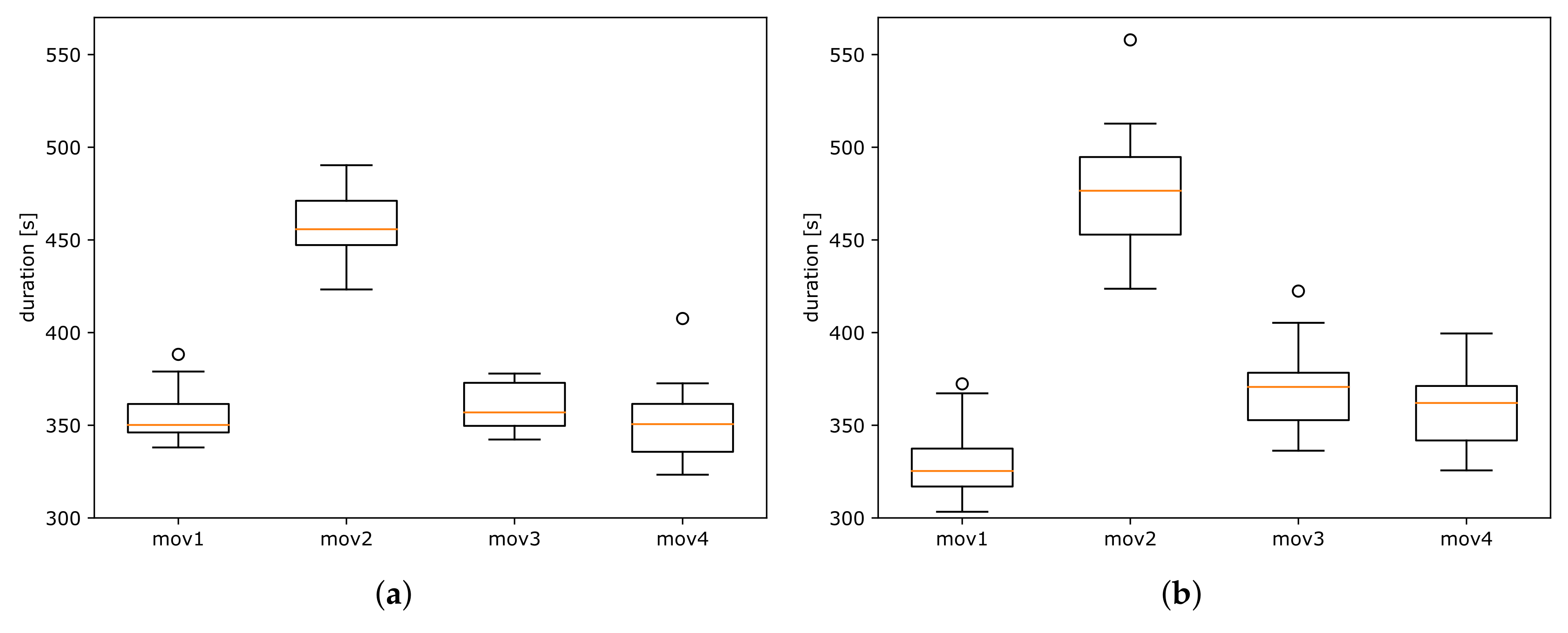
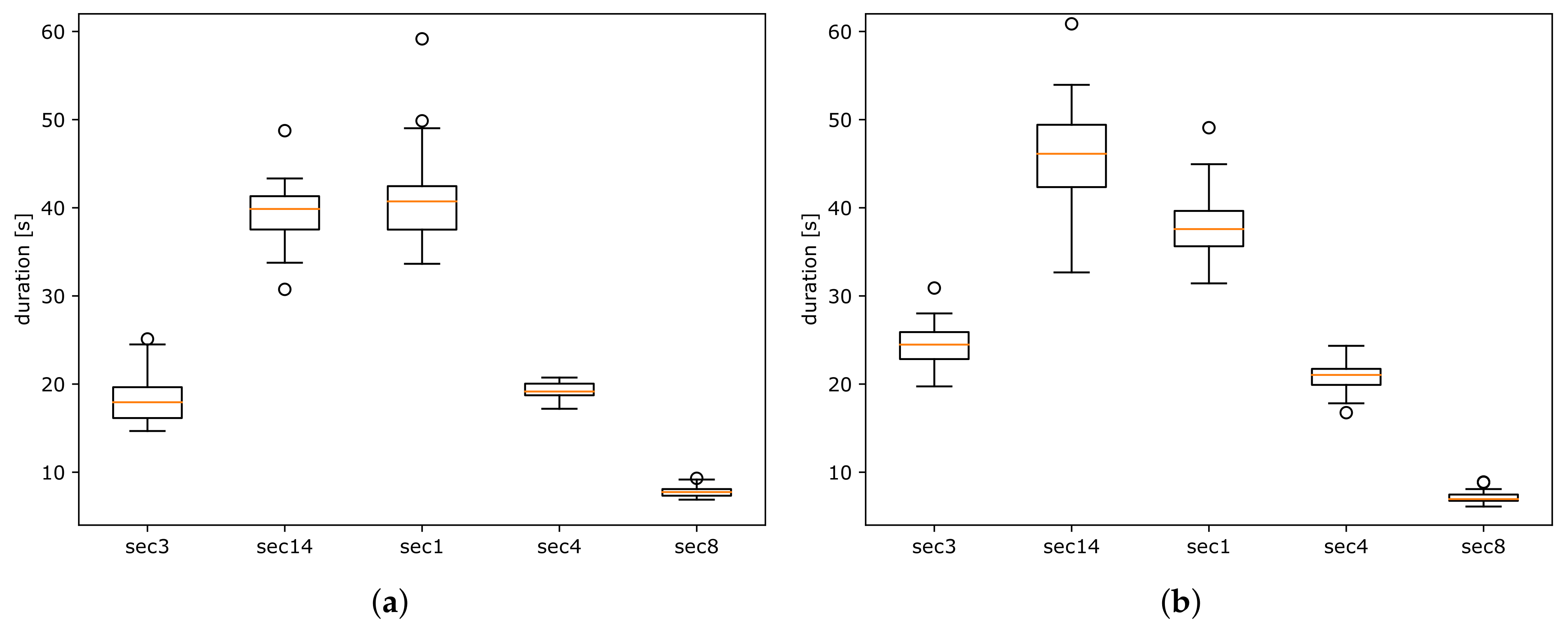
All features might describe specific qualities of a given performance, but in this paper, we chose only robust timing information for the origin classification. The duration of small time segments (such as measures) provides information about musical expressiveness and interpretive differences. If we choose larger segments, such as the duration of whole movements or sections composed of many measures, the significant differences and the accuracy of the potential classification decrease (compare Table 13 with Table 8 or Table 10). The exception is Janáček’s String Quartet No. 2, where we achieved F-measure = 0.87. Converting the duration to tempo values does not affect the classifier; it might only serve as a more intuitive visualization. We chose measures for a few reasons: firstly, measures are well-defined by the corresponding score; secondly, they are easier to annotate manually than, for example, beats; and thirdly, they can be used to segment recordings to sections or other logical structures (while ignoring the metrical structure of a given composition).

In Section 2.4, we show that automated downbeat tracking systems are not yet efficient for expressive string quartet music. Thus, the synchronization strategy (with available manual annotation) remains the preferable option. Feature selection explained in Section 3.2 helped the chosen classifier achieve higher accuracy while ranking the importance of features for a given task. This information can be further used for music analysis and a detailed comparison of differences. Using general structures such as measures has one more advantage—it allows us to generalize the classification pipeline to arbitrary music compositions, instruments, and genres.

The limitation of this study is the number of interpretations for given compositions. We collected a large dataset of string quartet recordings, but only a portion was used (see Section 2.3) due to the different music structures. To balance the data, we stratified the training and test subsets in each classification run, so there was always the same number of items in both classes. Considering compositions such as Janáček’s String Quartet No. 2, Dvořák’s String Quartet No. 13, or Smetana’s String Quartet No. 1, the classifier provides promising results, confirming the original idea that proposed classes (Czech and non-Czech interpretations) are distinguishable (see Table 13). However, if we use random labels, binary classification based on the duration of specific measures (given by the composition and all available interpretations) already provides relatively high accuracy in some cases. This is expected, as the mRMR method chooses 10 relevant features that distinguish these classes the most. If we do not implement a feature selection method, the classifier cannot be trained using the proposed strategy. The classification accuracy increases overall when we use the CZ and non-CZ labels.

This study shows that origin-based differences in interpretations exist and are measurable. However, the proposed machine learning pipeline cannot be universally used—the reference measure positions are always needed for at least one recording of a given composition, and we train and test the classifier for each composition separately. Thus far, we cannot classify the origin of arbitrary recording without prior knowledge of the piece and other interpretations. In the future, we would like to test the strategy on string quartets from, for example, Joseph Hayden or Ludwig van Beethoven with Austrian/German labels and provide a more detailed analysis of interpretation differences.

6. Conclusions

In this paper, we investigated the possibilities of string quartet interpretation classification based on performers’ origin. We collected a large dataset of string quartets from Czech composers Dvořák, Janáček, and Smetana. We manually annotated ground-truth measure positions of reference recordings and applied a method of time alignment to transfer measure positions to all target recordings. Furthermore, we used measures to segment recordings into separate sections and split our experiments into three scenarios, each specified by different features. We trained and tested a machine learning classifier to distinguish Czech and non-Czech interpretations of string quartet pieces. We showed that it is possible to train such a classifier. The classifier achieved poor results when feature matrices contained the duration of whole movements, except for Janáček’s String Quartet No. 2 with F-measure = 0.87. Increasing the time resolution of features, from movements to sections and measures, improved the prediction accuracy. For the third scenario, where measure positions were used, we achieved F-measure = 0.99 for Dvořák’s String Quartet No. 13, movements 3 and 4, and up to 0.96 in the case of Janáček’s String Quartet No. 2. Using proposed labels, the accuracy increased compared to the baseline with random labels, which already provided relatively high accuracy. It seems that interpretation-based differences are already distinguishable, in some cases, even in random subsets. In the future, we will experiment with other string quartet composers, use more labels, and further describe and explain the interpretation differences. We plan to experiment even with finer time resolution, such as beats, to train classifiers and identify differences in various interpretations.

References

1. Schedl, M.; Gómez, E.; Urbano, J. Music Information Retrieval: Recent Developments and Applications. Found. Trends Inf. Retr. 2014, 8, 127–261. [Google Scholar] [CrossRef] [Green Version]
2. Müller, M.; Pardo, B.A.; Mysore, G.J.; Välimäki, V. Recent Advances in Music Signal Processing [From the Guest Editors]. IEEE Signal Process. Mag. 2019, 36, 17–19. [Google Scholar] [CrossRef]
3. Lerch, A.; Arthur, C.; Pati, A.; Gururani, S. An Interdisciplinary Review of Music Performance Analysis. Trans. Int. Soc. Music Inf. Retr. 2021, 3, 221–245. [Google Scholar] [CrossRef]
4. Seddon, F.; Biasutti, M. A comparison of modes of communication between members of a string quartet and a jazz sextet. Psychol. Music 2009, 37, 395–415. [Google Scholar] [CrossRef]
5. Bishop, L.; Cancino-Chacón, C.; Goebl, W. Moving to Communicate, Moving to Interact: Patterns of Body Motion in Musical Duo Performance. Music Percept. 2019, 37, 1–25. [Google Scholar] [CrossRef] [Green Version]
6. Papiotis, P.; Marchini, M.; Perez-Carrillo, A.; Maestre, E. Measuring ensemble interdependence in a string quartet through analysis of multidimensional performance data. Front. Psychol. 2014, 5, 963. [Google Scholar] [CrossRef] [Green Version]
7. Tzanetakis, G.; Cook, P. Musical Genre Classification of Audio Signals. IEEE Trans. Audio Speech Lang. Process. 2002, 10, 293–302. [Google Scholar] [CrossRef]
8. Seyerlehner, K.; Schedl, M.; Pohle, T.; Knees, P. Using Block-Level Features for Genre Classification, Tag Classification and Music Similarity Estimation. Available online: http://www.cp.jku.at/people/schedl/Research/Publications/pdf/MIREX_SSPK2_2010.pdf (accessed on 6 November 2022).
9. Mo, S.; Niu, J. A novel method based on OMPGW method for feature extraction in automatic music mood classification. IEEE Trans. Affect. Comput 2017, 10, 313–324. [Google Scholar] [CrossRef]
10. Liebman, E.; Ornoy, E.; Chor, B. A Phylogenetic Approach to Music Performance Analysis. J. New Music Res. 2012, 41, 195–222. [Google Scholar] [CrossRef]
11. Hillewaere, R.; Manderick, B.; Conklin, D. String Quartet Classification with Monophonic Models. In Proceedings of the 11th International Society for Music Information Retrieval Conference (ISMIR), Utrecht, The Netherlands, 9–13 August 2010. [Google Scholar]
12. Kempfert, K.C.; Wong, S.W. Where does Haydn end and Mozart begin? Composer classification of string quartets. J. New Music Res. 2020, 49, 457–476. [Google Scholar] [CrossRef]
13. Lykartsis, A.; Lerch, A. Beat Histogram Features for Rhythm-Based Musical Genre Classification Using Multiple Novelty Functions. In Proceedings of the 18th International Conference on Digital Audio Effects (DAFx-15), Trondheim, Norway, 30 November–3 December 2015. [Google Scholar]
14. Kiska, T.; Galáž, Z.; Zvončák, V.; Mucha, J.; Mekyska, J.; Smékal, Z. Music Information Retrieval Techniques for Determining the Place of Origin of a Music Interpretation. In Proceedings of the 10th International Congress on Ultra Modern Telecommunications and Control Systems and Workshops (ICUMT), Moscow, Russia, 5–9 November 2018. [Google Scholar]
15. Bowen, J.A. Tempo, duration, and flexibility: Techniques in the analysis of performance. J. Musicol. Res. 1996, 16, 111–156. [Google Scholar] [CrossRef]
16. Cook, N. Analysing performing and performance analysis. In Rethinking Music, New ed; Oxford University Press: Oxford, UK, 1999; Chapter 11; pp. 239–261. [Google Scholar]
17. Sapp, C.S. Comparative Analysis of Multiple Musical Performances. In Proceedings of the 8th International Conference on Music Information Retrieval (ISMIR), Vienna, Austria, 23–27 September 2007; pp. 497–500. [Google Scholar]
18. Cancino-Chacón, C.E.; Grachten, M.; Goebl, W.; Widmer, G. Computational models of expressive music performance: A comprehensive and critical review. Frontiers Digit. Humanit. 2018, 5, 25. [Google Scholar] [CrossRef] [Green Version]
19. Cancino-Chacón, C.E.; Gadermaier, T.; Widmer, G.; Grachten, M. An Evaluation of Linear and Non-linear Models of Expressive Dynamics in Classical Piano and Symphonic Music. Mach. Learn. 2017, 106, 887–909. [Google Scholar] [CrossRef] [Green Version]
20. Chacón, C.E.C.; Bonev, M.; Durand, A.; Grachten, M.; Arzt, A.; Bishop, L.; Goebl, W.; Widmer, G. The ACCompanion v0.1: An expressive accompaniment system. In Proceedings of the In Late Breaking Demo, 18th International Society for Music Information Retrieval Conference (ISMIR 2017), Suzhou, China, 23–27 October 2017. [Google Scholar]
21. Xia, G.; Wang, Y.; Dannenberg, R.; Gordon, G. Spectral learning for expressive interactive ensemble music performance. In Proceedings of the International Society for Music Information Retrieval Conference (ISMIR), Malaga, Spain, 26–30 October 2015; pp. 816–822. [Google Scholar]
22. Henkel, F.; Balke, S.; Dorfer, M.; Widmer, G. Score Following as a Multi-Modal Reinforcement Learning Problem. Trans. Int. Soc. Music. Inf. Retr. 2019, 2, 66–81. [Google Scholar] [CrossRef]
23. Cancino-Chacón, C.E.; Grachten, M. The Basis Mixer: A Computational Romantic Pianist. In Proceedings of the Late Breaking/Demo Session. In Proceedings of the Late Breaking/Demo Session, 17th International Society for Music Information Retrieval Conference (ISMIR 2016), New York, NY, USA, 7–11 August 2016. [Google Scholar]
24. Schlüter, J. Deep Learning for Event Detection, Sequence Labelling and Similarity Estimation in Music Signals. Ph.D. Thesis, University Linz, Linz, Austria, 2017. [Google Scholar]
25. Müller, M.; Özer, Y.; Krause, M.; Prätzlich, T.; Driedger, J. Sync Toolbox: A Python Package for Efficient, Robust, and Accurate Music Synchronization. J. Open Source Softw. 2021, 6, 3434. [Google Scholar] [CrossRef]
26. Ewert, S.; Muller, M.; Grosche, P. High resolution audio synchronization using chroma onset features. In Proceedings of the IEEE International Conference on Acoustics, Speech and Signal Processing (ICASSP), Taipei, Taiwan, 19–24 April 2009. [Google Scholar]
27. Lerch, A. Software based extraction of objective parameters from music performances. Ph.D. Thesis, Technischen Universitat Berlin, Berlin, Germany, 2009. [Google Scholar]
28. Weiß, C.; Arifi-Müller, V.; Prätzlich, T.; Kleinertz, R.; Müller, M. Analyzing Measure Annotations for Western Classical Music Recordings. In Proceedings of the 17th International Society for Music Information Retrieval Conference (ISMIR), New York City, NY, USA, 7–11 August 2016. [Google Scholar]
29. Müller, M.; Kurth, F.; Clausen, M. Audio Matching via Chroma-Based Statistical Features. In Proceedings of the 6th International Conference on Music Information Retrieval (ISMIR), London, UK, 11–15 September 2005. [Google Scholar]
30. Prätzlich, T.; Driedger, J.; Müller, M. Memory-Restricted Multiscale Dynamic Time Warping. In Proceedings of the 41st IEEE International Conference on Acoustics, Speech and Signal Processing (ICASSP), Shanghai, China, 20–25 March 2016. [Google Scholar]
31. Böck, S.; Krebs, F.; Widmer, G. Joint Beat and Downbeat Tracking with Recurrent Neural Networks. In Proceedings of the 17th International Society for Music Information Retrieval Conference (ISMIR), New York City, NY, USA, 7–11 August 2016. [Google Scholar]
32. Steinmetz, C.J.; Reiss, J.D. WaveBeat: End-to-end beat and downbeat tracking in the time domain. In Proceedings of the 151st Audio Engineering Society Convention, Las Vegas, NV, USA, 13 October 2021. [Google Scholar]
33. Böck, S.; Cardoso, J.S.; Davies, M.E.P. Deconstruct, Analyse, Reconstruct: How to improve Tempo, Beat, and Downbeat Estimation. In Proceedings of the 21st International Society for Music Information Retrieval Conference (ISMIR), Virtual, 11–16 October 2020. [Google Scholar]
34. Raffel, C.; McFee, B.; Humphrey, E.J.; Salamon, J.; Nieto, O.; Liang, D.; Ellis, D.P.W. MIR_EVAL: A Transparent Implementation of Common MIR Metrics. In Proceedings of the 15th International Society for Music Information Retrieval Conference (ISMIR), Taipei, Taiwan, 27–31 October 2014. [Google Scholar]
35. Davies, M.E.; Degara, N.; Plumbley, M.D. Evaluation Methods for Musical Audio Beat Tracking Algorithms; Technical Report; Queen Mary University of London, Centre for Digital Music: London, UK, 2009. [Google Scholar]
36. Pinto, A.S.; Böck, S.; Cardoso, J.S.; Davies, M.E.P. User-Driven Fine-Tuning for Beat Tracking. Electronics 2021, 10, 1518. [Google Scholar] [CrossRef]
37. Ištvánek, M.; Miklánek, Š. Exploring the Possibilities of Automated Annotation of Classical Music with Abrupt Tempo Changes. In Proceedings of the 28th Student EEICT 2022, Brno, Czech Republic, 16 April 2022. [Google Scholar]
38. Pinto, A.S.; Domingues, I.; Davies, M.E.P. Shift If You Can: Counting and Visualising Correction Operations for Beat Tracking Evaluation. arXiv 2020, arXiv:2011.01637. [Google Scholar]
39. Ištvánek, M.; Miklánek, Š. Towards Automatic Measure-Wise Feature Extraction Pipeline for Music Performance Analysis. In Proceedings of the 45th International Conference on Telecommunications and Signal Processing (TSP), Virtual, 13–15 July 2022. [Google Scholar]
40. Ding, C.; Peng, H. Minimum Redundancy Feature Selection from Microarray Gene Expression Data. J. Bioinform. Comput. Biol 2003, 3, 185–205. [Google Scholar] [CrossRef]
41. Zhao, Z.; Anand, R.; Wang, M. Maximum Relevance and Minimum Redundancy Feature Selection Methods for a Marketing Machine Learning Platform. In Proceedings of the 6th IEEE International Conference on Data Science and Advanced Analytics (DSAA), Washington, DC, USA, 5–8 October 2019. [Google Scholar]
42. Drotár, P.; Mekyska, J.; Rektorová, I.; Masarová, L.; Smékal, Z.; Faundez-Zanuy, M. Analysis of in-air movement in handwriting: A novel marker for Parkinson’s disease. Comput. Methods Programs Biomed. 2014, 117, 405–411. [Google Scholar] [CrossRef]
43. Li, B.Q.; Hu, L.L.; Chen, L.; Feng, K.Y.; Cai, Y.D.; Chou, K.C. Prediction of Protein Domain with mRMR Feature Selection and Analysis. PLoS ONE 2012, 7, e39308. [Google Scholar] [CrossRef] [Green Version]
44. Peng, H.; Long, F.; Ding, C. Feature Selection Based on Mutual Information Criteria of Max-Dependency, Max-Relevance, and Min-Redundancy. IEEE Trans. Pattern Anal. Mach. Intell. 2005, 27, 1226–1238. [Google Scholar] [CrossRef] [PubMed]
45. Chang, C.C.; Lin, C.J. LIBSVM: A library for support vector machines. ACM Trans. Intell. Syst. Technol. 2011, 2, 1–27. [Google Scholar] [CrossRef]
46. Schölkopf, B.; Smola, A.J.; Williamson, R.C.; Bartlett, P.L. New Support Vector Algorithms. Neural Comput. 2000, 12, 1207–1245. [Google Scholar] [CrossRef] [PubMed]
47. Cortes, C.; Vapnik, V. Support-Vector Networks. Mach. Learn. 1995, 20, 273–297. [Google Scholar] [CrossRef]
Figure 1. Overview of the proposed classification strategy.
Applsci 13 03603 g001
Figure 2. An example of a warping path between a reference and a target recording; interpretations differ in the underlying musical structure (the target recording contains measures that are not included in the reference recording); blue dots correspond to the anchor points; blue line shows the diagonal path between anchor points; green points (crosses) are projected on the warping path and are equally distributed; red points (crosses) indicate the region of a dissimilarity because their τ r > 3.
Applsci 13 03603 g002
Figure 3. The boxplots of the first scenario for Janáček’s String Quartet No. 2 show both proposed classes’ statistics and data distribution. (a) The boxplot of class 1 (CZ); (b) the boxplot of class 0 (non-CZ).
Applsci 13 03603 g003
Figure 4. The boxplots of the second scenario for Janáček’s String Quartet No. 2, movement 2, show both proposed classes’ statistics and data distribution. (a) The boxplot of class 1 (CZ); (b) the boxplot of class 0 (non-CZ).
Applsci 13 03603 g004
Figure 5. The boxplots of the third scenario for Dvořák’s String Quartet No. 13, movement 3, show both proposed classes’ statistics and data distribution. (a) The boxplot of class 1 (CZ); (b) the boxplot of class 0 (non-CZ).
Applsci 13 03603 g005