Abstract
This paper proposes a new hybrid algorithm for grey wolf optimization (GWO) integrated with a robust learning mechanism to solve the large-scale economic load dispatch (ELD) problem. The robust learning grey wolf optimization (RLGWO) algorithm imitates the hunting behavior and social hierarchy of grey wolves in nature and is reinforced by robust tolerance-based adjust searching direction and opposite-based learning. This technique could effectively prevent search agents from being trapped in local optima and also generate potential candidates to obtain a feasible solution. Several constraints of power generators, such as generation limits, local demand, valve-point loading effect, and transmission losses, are considered in practical operation. Five test systems are used to evaluate the effectiveness and robustness of the proposed algorithm in solving the ELD problem. The simulation results clearly reveal the superiority and feasibility of RLGWO to find better solutions in terms of fuel cost and computational efficiency when compared with the previous literature.
1. Introduction
Economic load dispatch (ELD) is considered the most elementary and computationally heavy optimization problem in electricity industry studies. ELD enables the power system to analyze the committed generating units to allocate the optimum level of active power output to achieve the total power demands at the cheapest operating cost while satisfying several physical and operational constraints [1]. Over the last few years, various mathematical programming techniques and optimization methods have been applied to solve ELD problems, such as the Newton method [2], the gradient method [3], the base point and participation factors method, and the Lambda-iteration method [2]. Nevertheless, none of the mentioned techniques perform well in addressing practical problems with nonlinear and discontinuous characteristics since these methods required the incremental cost of the generators to be increase in a monotonic or piecewise linear fashion [2]. Therefore, nonlinear programming [4], dynamic programming [5], and some of their modified applications have been employed to deal with ELD issues. Unfortunately, the drawback of these methods is their computational time, which when applied to modern power systems with a huge number of generating units is too long.
To overcome the downside of traditional mathematical programming, researchers around the world have introduced metaheuristic optimization algorithms, such as simulated annealing (SA) [6], genetic algorithms (GAs) [7], tabu searches (TS) [8], and artificial neural networks (ANNs) [9]. Yalcinoz [10] successfully addressed complex optimization issues. However, these probabilistic heuristic algorithms do not always guarantee the global search property. Recently, different kinds of global optimization algorithms have been proposed, such as particle swarm optimization (PSO) [11], modified particle swarm optimization [12], biogeography-based optimization (BBO) [13], modified genetic algorithm [14], bacteria foraging optimization [15], differential evolution (DE) [16], and ant colony optimization [17]. The application of these techniques in ELD has delivered some promising solutions in terms of minimizing total generation cost and improving convergence rate.
However, recent research has recognized a few deficiencies in stochastic algorithms like GA. This degradation in efficiency and limited search capability may be noticeable when applied to multimodal objective functions. Additionally, TS requires a suitable selection of control parameters to attain an optimal solution. Slow convergence can be considered a key disadvantage of GA, SA, TS, and ANN, making them unable to appropriately address real-time issues. Even though PSO has attracted research interest due to its rapid convergence characteristic and its flexibility, PSO is still restricted when applied to large-scale real-time ELD, since it is not always guaranteed that the total generation cost is the global best solution.
The modification of the presented algorithm can be a solution for achieving the global optimal solution and upgrading the convergence rate. Existing modified metaheuristic methods include chaotic differential evolution and sequential quadratic programming (DEC_SQP) [18], improved coordinated aggregation-based PSO (ICA_PSO) [19], quantum-inspired particle swarm optimization (QPSO) [20], modified shuffled frog leaping algorithm with GA crossover (MSFLA and GA) [21], a different version of PSO [19], shuffled differential evolution (SDE) [21], hybrid biogeography-based optimization with differential evolution (DE/BBO) [22], and adaptive hybrid backtracking search optimization [23]. Oppositional invasive weed optimization (OIWO) [24] improves the convergence rate of invasive weed optimization by incorporating opposite-based learning (OBL) [25]. Nevertheless, this OIWO relies heavily on the initial selection of control parameters to obtain the global best solution. Moreover, the solution is not unique for every trial, and this method also has the problem of long computational time.
In recent years, a new evolutionary optimization technique, called grey wolf optimization (GWO), which mimics the social hierarchy and hunting behavior of grey wolves, has been proposed by Mirjalili et al. [26]. There are several applications of GWO in power system optimization problems [27,28]. The outstanding characteristic of GWO compared with other stochastic heuristic algorithms is that it does not depend on accurate initialization of input parameters to obtain the global best solution. However, the parameters still need to be modified to avoid premature convergence, as well as to improve the convergence speed. To overcome the above limitation, a hybrid GWO algorithm with a robust learning mechanism (RLGWO) is introduced in this paper that incorporates opposite-based learning (OBL) as a candidate generation strategy. The main reason for selecting OBL is that it does not require any specific technique to speed up the convergence rate of different optimization algorithm. Additionally, the candidates generated by OBL are more likely to come closer to the global optimum solution than a solution using randomly generated candidates, because the technique simultaneously considers both the current population and its opposite. In only a short period of time, OBL, a new concept in computational intelligence, has attracted research attention with the aim of enhancing metaheuristic optimization algorithms to address large-scale ELD [24,29].
In this paper, the performance of a proposed grey wolf algorithm variant with robust tolerance-based adjust searching direction mechanism (RTASDM), called the robust learning grey wolf algorithm (RLGWO), is studied. The algorithm is tested on five test systems with different sizes and in consideration of power system constraints to evaluate the performance of the proposed approach in solving the ELD problem compared with other variants of the GWO. The reported results reveal the ability of RLGWO to archive superior solutions in terms of quality, consistency, and convergence rate compared to several other optimization methods.
2. Problem Formulation
Economic load dispatch is a classical optimization problem in power systems. The main goal is to obtain the cheapest fuel cost by allocating the optimal power output among the available generating units while satisfying various equality and inequality constraints.
2.1. Objective Function
The main objective of the ED problem is to minimize the total generation costs of a power system by determining the power output of generators that satisfies various constraints, such as the load demands of PD are met within an appropriate period (normally in one hour), the active balance constraint, and the limitation of the generator. The simplified cost function of ED can be written as:
where is the total generation cost, is the cost function of the ith generating unit in terms of , which is the power output of ith generating unit. , and are the fuel cost coefficients of ith generating unit. Finally, is the total number of generating units.
Practically, the generators with multiple valve steam turbines exhibit a wide variation with respect to the fuel cost function. This is because the valve-point creates a ripple, whereby the cost function cannot be represented by a quadratic polynomial function as in (2), since it contains nonlinear characteristics. Therefore, the cost function considered in this paper is a combination of quadratic functions and sinusoidal functions, which are represented as follows:
where and are the constants of the ith generating unit reflecting the valve-point effect [30].
Additionally, thermal dispatching units are realistically supplied from different fuel sources with several types of fuel. The operation of each dispatching unit should be mathematically represented under multiple piecewise functions to emphasize the effect of multiple fuel sources. Both the valve-point effect and multiple fuel options should be combined to acquire a practical and reliable ELD. Finally, the cost function of the ith generating unit can be realistically expressed as below:
2.2. Equality and Inequality Constraints
- (a)
- Active power balance constraintThe total generated power output should be the same as the sum of the total power demand and the total system loss . This is represented as follows:
- (b)
- The limitations of the generatorThe power output of each generating unit should be limited to between its minimum and maximum power outputs, as shown in the inequality constraint in (6):where and are the minimum and maximum real power output of the generating unit i.
3. GWO Algorithm
The Grey Wolf Optimizer (GWO) was modeled by Mirjalili et al. [26] based on the social hierarchy and the hunting behavior of grey wolves.
3.1. Social Hierarchy
The grey wolf belongs to the Canidae family, and they are considered to be apex predators, which means that they are at the top of the food chain. They mostly prefer to live in packs, and they have a very strict social dominance hierarchy, consisting of alpha, beta, delta, and omega [26].
To mathematically model the GWO based on the social hierarchy characteristics of wolves, the alpha (α) is considered to be the fittest solution. The beta (β) and the delta (δ) are consequently utilized as the second- and third-best solutions, respectively. The omega (ω) corresponds to the remainder of the candidate solutions. The hunting (optimization) in the GWO algorithm is guided by α, β, and δ. The ω follows these three leaders.
3.2. Encircling Prey
Group hunting is another interesting social behavior that emphasizes the social hierarchy of grey wolves, as described above. According to Muro et al. [31], the hunting process of grey wolves includes three main steps: (1) tracking, chasing, and approaching the prey; (2) encircling, pursuing, and harassing the prey until it stops moving; and (3) attacking the prey. The following equations show the mathematical modeling of encircling behavior [26]:
where is the position vector of the prey, is the position vector of the grey wolf, t indicates the current iteration, and are coefficient vectors.
The vectors and are calculated as follows:
where decreases linearly from 2 to 0 over the course of multiple iterations, and , are random vectors [0,1].
3.3. Hunting
The alpha, beta, and delta are assumed to have the ability to recognize potential locations of prey, since they hold the three best solutions obtained so far. Hence, their solution positions are utilized to update the positions of all of the other (omega) wolves. The updated position formulation proposed above is as follows:
After repeatedly applying the encircling and hunting techniques, the prey (the fittest solution) will be located.
4. Robust Learning-Based GWO Algorithm (RLGWO)
All omega members of the hunting group in the original GWO learn from the first three best leaders to update their position until the termination condition is reached, even if the fittest solution (alpha) is trapped in a local optimum. This kind of learning algorithm can work well in the exploitation phase and has the ability to converge rapidly, but is invalid when solving problems with such large and complex search spaces. Some methods have been proposed for GWO incorporating strategies to restrict the learning mechanism of omega to maintain the diversity of the population, like EEGWO [32] and GWO-ABC [33]. These strategies result in good exploration performance. However, it takes a longer time to reach a solution and slows down the convergence rate of the algorithm.
The algorithm (RLGWO) proposed in this paper achieves a balance between exploitation and exploration. In RLGWO, a robust tolerance-based adjust searching direction mechanism is used. This method gives omega the ability to adjust their search direction to avoid falling into local optima and to diminish the size of the search space. Additionally, an opposition learning-based candidate grey wolf strategy is utilized to generate candidate leaders that replace the position of alpha as well as beta and delta, in which the hunting group can perform in different areas within the search space. Subsequently, looking toward guaranteeing the efficiency and accuracy of the algorithm, a potential position update scheme is introduced to adapt the potential ability of the candidate leader to guide the grey wolf for exploitation in divergent dimensions.
4.1. Robust Tolerance-Based Adjust Searching Direction Mechanism (RTASDM)
It is widely known that the grey wolf in the original GWO had a high possibility of getting stuck in local optima when operating in a large and complex search space. In Figure 1a, the hunting mechanism for a one-dimensional problem is presented, where the blue curve illustrates the object function. is the alpha position (the best solution) that leads the rest of the population. In Figure 1a, it is clear that each omega can move along the guiding direction of the alpha fitness value and the hunting group will be trapped in a local optimum after several iteration. Assume indicates the objective value of the nth omega in the population at the kth iteration. will be updated in the next iteration using Formula (13). Then, it will generate a new fitness denoted by . The total difference between and in the population can be described as shown in (14), where N is the population size.
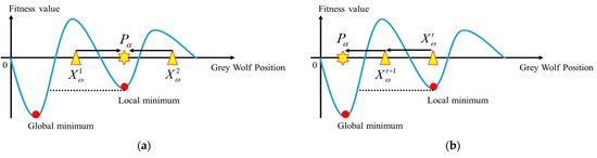
Figure 1.
The hunting mechanism of GWO in one-dimensional minimization. (a) falls into a local optimum; and (b) reaches the global optimum..
After the course of iteration, the solution may finally converge to the optimum solution (global or local optimum). This situation indicates that is more likely to be close to 0. Assuming that is a small value around 0, we can determine when the hunting group is going to converge by setting that belongs to a range of . Therefore, Formula (14) can be rewritten as:
To avoid the hunting groups getting stuck in the local optimum and to ensure the efficiency of the algorithm, the omega’s search direction can be adjusted every time Equation (15) is satisfied. Nevertheless, when dealing with a large and complex space, we cannot rely on the circumstances described above to change the search direction of the omega. It can be clearly seen in Figure 1b that when the alpha position (global best solution) gets close to the global optimum, it leads the other members of the hunting group to search in the direction towards . This also means that the solution of the generation may not be improved by the alpha, while also satisfying the conditions shown in Equation (15). Therefore, depending on the potential ability of , the hunting group can be led to a promising global optimum over the next few iterations [34].
After several iterations, as the number of satisfied conditions increases, meaning that there is no difference between the current solution and previous solutions, it can be concluded that the grey wolf is stuck around a local optimum. Therefore, the grey wolf needs to modify its search direction. Let be a tolerance variable, where is initially set to 0 and is used as a counter. In cases where (15) is satisfied, can be updated via Equation (16), as follows.
As the value of becomes greater, the probability of becoming trapped in the local optima of a hunting group also increases [34]. However, in cases where is searching around the global optimum, as described above, the omega should not change their search direction, but rather move along the alpha direction. Therefore, we introduce the probability , which enables the omega to adjust its search direction. can be achieved experimentally using Equation (17), below, where is the current iteration and is the maximum number of iterations.
As can be seen from Figure 2, the is not fixed throughout the course of iterations; rather, its value is updated according to and . When the value of is larger than a random number with a range of [0,1], the leader alpha (beta or gamma) will be replaced by another candidate solution, which will continue to guide the hunting group.
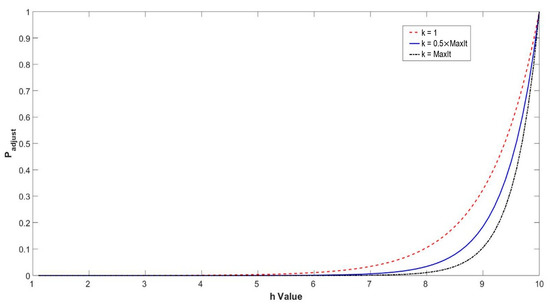
Figure 2.
Adjustment probability at different iteration periods.
Algorithm 1, below, shows the details of the approach.
| Algorithm 1. Robust tolerance-based adjust searching direction mechanism |
| 1: At iteration kth; |
| then |
| 5: end if |
| 6: generate a random number in the range of [0,1]; |
| then |
| 8: Finding another candidate solution to replace alpha (beta or gamma) |
| 9: end if |
It is clear from Figure 2 and Algorithm 1 that the depends on and , especially the tolerance value . When the value of is small, has a high probability of becoming smaller than the random number; then, the first three best leaders continue to guide the hunting group, and their leading ability will be useful for the next several iterations. When increases to the threshold, increases dramatically. This indicates that the number of solutions has still not improved over the next several iterations, and the hunting group is more likely to become trapped in a local optimum. Therefore, the value of is probably greater than the random number, and a new leader will be used to lead the omega search direction.
On top of that, is more likely to get close to the global optimum when the number of iterations is increased, especially with numbers of iterations greater than half, as can be seen in Figure 3. Therefore, to ensure convergence, the value of should be increased to get rid of the omega and change its search direction.
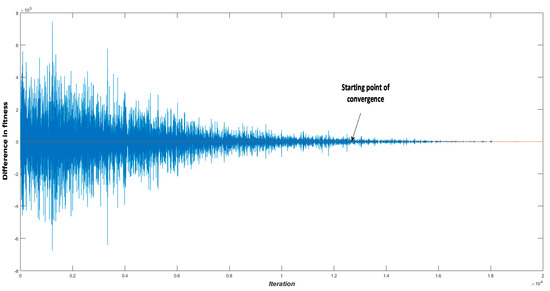
Figure 3.
The convergence rate of the search mechanism.
4.2. Opposition-Based Learning for Candidate Generation Strategy
Opposition-based learning (OBL) [25] has recently been utilized to accelerate the convergence rate of several optimization algorithms. The OBL technique can be used to generate potential candidate solutions by considering both the current population and its opposite population. It has been proved in many studies worldwide that opposition candidate solutions are more likely to get closer to the global optimum solution than a randomly generated candidate solution. There have been many advanced applications of this learning mechanism in several soft computing techniques, as reported in [35,36,37,38].
The two definitions below show the important aspects of OBL, the opposite number and opposite point [25]:
Definition—Let be a real number defined in a certain interval: . The opposite number is defined as follows:
Definition—Let be a point in an n-dimensional coordinate system with and . The opposition point is completely defined by its coordinates where
In the proposed RLGWO, after defining the replacement of the leader with a candidate solution in Section 4.1, a random candidate solution can easily be created in the search space to guide the hunting group to get rid of the current local optimum solution. However, the random candidate may not be guaranteed to improve the solution; in particular, when dealing with large and complex spaces, it is probable that it will lead the hunting group into another local optimum. Using the OBL can ensure the generation of a candidate more effectively.
In Figure 3, it is clear to see that the difference between the current and the previous solution in the first half of the iteration changes violently. This circumstance can be explained by the fact that the hunting group is carrying out the exploration phase. This means that the grey wolves are attempting to search the hold space to figure out promising areas for the global optimum. The alpha will have a significant influence on the hunting group, since it is the best solution. Therefore, in this certain period, replacing the alpha with its opposite position is a wise course of action to escape the local optimum.
The remaining half of the total course of iteration is the exploitation phase, when the grey wolf scales down the search space and concentrates on a certain area to find the optimum solution. To prevent the omega from moving away from the global optimum and to ensure the efficiency of the algorithm, the alpha acts as the main leader and the beta (or gamma) may be replaced by its opposite position. Since the beta and gamma have almost the same potential ability, the beta will be removed if the random number is greater than 0.5, and conversely, gamma will be substituted if it is less than this value.
The details of the generating candidate are described in Algorithm 2.
| Algorithm 2. Opposition-based learning for candidate generation strategy |
| 1: At iteration kth; |
| between [0,1]; |
| 4: Keep alpha, beta, and gamma as the leader; |
| 5: else |
| then |
| ; |
| 8: else |
| between [0,1]; |
| ; |
| 12: else |
| ; |
4.3. RLGWO Algorithm for Economic Load Dispatch
The computational mechanism for the proposed RLGWO algorithm to solve ELD problems is described in the following steps.
Step 1. Initialization
Step 1.1: Arbitrarily generate the initial value for all of the active power of the generating units belonging to their lower and upper real power operating limits except the last unit. Equation (4) is used to compute the amount of active power output of the last unit to guarantee whether it satisfies the inequality constraint or not. The solution will be discarded whenever it violates the inequality constraint. Let D be the dimension of the hunting group. The initial position of the grey wolves is given as a matrix, , below:
Step 1.2: Substitute the matrix into (3) and calculate the fuel cost for each solution of the current population.
Step 1.3: Evaluate the cost value of all search agents (grey wolves), which determine , , as the first three best solutions by simple comparison of their cost value.
Step 1.4: Set all the parameters, including , , coefficient vector and , initial variable tolerance .
Step 2. Repeat this step until the stopping criterion is satisfied.
Step 2.1: Update the position of all search agents using (11)–(13).
Step 2.2: Calculate the fuel cost for all members of the hunting group using (3) and compare the results to figure out , , .
Step 2.3: Evaluate , and then check whether fulfills Condition (15) or not. In cases where belongs to the range , will be increased by 1.
Step 2.4: Compute the probability of using (17) and select a random number . If , meaning that the three best leaders still potentially have the ability to guide all search agents, then return to Step 2. Otherwise, follow Algorithm 2 to generate a suitable candidate to lead the hunting group and move back to Step 2.
5. Simulation Results and Discussion
Five different benchmark test systems were applied to evaluate the performance of the proposed RLGWO algorithm. Its performance was also compared with that of several optimization techniques reported in the literature. The nature-inspired RLGWO was executed using MATLAB 7.1 (R2010a) on Intel (R) 1GB RAM, 2.60 GHz CPU.
Dissimilar to other metaheuristic computations that require suitable values for the algorithm’s input parameters in order to improve their convergence rate, like particle swarm optimization (PSO) or evolutionary algorithms (ED), GWO has the advantage of being free from the initialization of input parameter. In this paper, the initial parameter for population size and the maximum number of iterations is selected as 50 and 200, respectively.
5.1. Test Systems and Results
5.1.1. Test System 1
This system contained 13 thermal units with a fuel cost function having a valve-point effect is used. The power demand, in this case, it is assumed to be 2520 MW, including transmission losses. The detailed parameters of the system were adopted from [24]. The solution obtained from the proposed RLGWO is compared with oppositional real coded chemical reaction optimization (ORCCRO) [29], a different version of PSO [19], shuffled differential evolution (SDE) [39], biogeography-based optimization (BBO) [13], DE/BBO [22], and OIWO [24], where Table 1 shows their best results. The convergence characteristic of the 13-unit test systems with the original GWO and RLGWO algorithms for fitness value are presented in Figure 4. This shows that the result of RLGWO is lower than the result of GWO.

Table 1.
Best simulation results of the 13-unit system with loss ( MW).
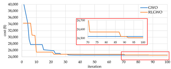
Figure 4.
Comparative convergence characteristic of original GWO and proposed RLGWO algorithm for the 13-unit system.
The statistical results of RLGWO and other published algorithms are listed in Table 2, showing the maximum, minimum, and average cost obtained using different methods over 50 trials. Figure 5 shows a visualization of the results presented in Table 2 of the different algorithms. The box graphs in Figure 5a show that the RLGWO always produces one of the lowest results for this problem. The ICA-PSO, on the other hand, has result statistics that are scattered over a wider range of cost. Figure 5b shows the time and number of hits of the minimum result. The RLGWO computational time is one of the fastest, with one of the highest number of hits to its minimum solution.
Table 2.
Comparison between different methods taken after 50 trials (13-unit system with loss).
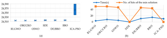
Figure 5.
Results for different methods for the 13-unit system (50 trials): (a) boxplot of the final generation cost; (b) time and number of hits of the minimum solution.
5.1.2. Test System 2
The medium-size ELD problem with 40 thermal units with the valve-point loading effect and transmission loss is considered. The total power demand is 10,500 MW, with input data taken from [24]. The total power output and fuel cost were determined for the 40-unit systems using several metaheuristic techniques, including OIWO [24], BBO [13], DE/BBO [22], SDE [39], and GAAPI [40], alogn with the proposed RLGWO, and the results are given in Table 3. A comparison of the convergence characteristics of the 40-unit system between the original GWO and RLGWO algorithms with respect to fitness value is shown in Figure 6. The magnified results in Figure 6 show that RLGWO obtained a lower cost for this system.
Table 3.
Best simulation results for the 40-unit system with loss ( MW).
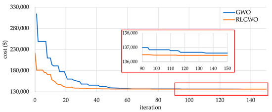
Figure 6.
Comparative convergence characteristics of the original GWO and the proposed RLGWO algorithms for the 40-unit system.
Table 4 presents the maximum, minimum, and average fuel cost obtained using the RLGWO, DE/BBO, SDE, OIWO, and GAAPI methods over 50 trials. These results are visualized in Figure 7. The OIWO produced the lowest and densest results of the five algorithms, as seen in Figure 7a. The RLGWO was second in terms of identifying the lowest cost, but was still always able to identify the lowest cost. As seen in Figure 7b, RLGWO and ORCCRO found the minimum result 50 times among 50 trials, but the solution found by ORCCRO was higher than that determined using RLGWO. Furthermore, RLGWO found the solution the fastest among the five algorithms.
Table 4.
Comparison between different methods taken after 50 trials (40-unit system with loss).
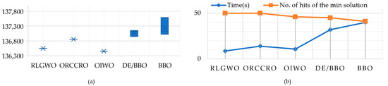
Figure 7.
Results for different methods for the 40-unit system (50 trials): (a) boxplot of the final generation cost; (b) time and number of hits of the minimum solution.
5.1.3. Test System 3
A test system with 110 generating units possessing quadratic fuel cost characteristics is utilized. The details of the input parameters were taken from [41]. The load demand is assumed to be 15,000 MW. The best solution obtained by the proposed RLGWO can be seen in Table 5. A comparison of the convergence characteristics of 110 generators between the GWO and RLGWO methods with respect to fitness value is presented in Figure 8.
Table 5.
Best simulation results for the 110-unit system with loss ( MW).
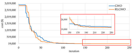
Figure 8.
Comparative convergence characteristics of the original GWO and the proposed RLGWO algorithms for the 110-unit system.
The maximum, minimum, and average achieved over 50 trials are given in Table 6. Figure 9 presents a visualization of Table 6. The RLGWO produced the lowest cost among the five algorithms and was able to find the minimum cost the most times (as can be seen from Figure 9b). Still, it is the fastest algorithm among the five algorithms tested.
Table 6.
Comparison between different methods taken after 50 trials (110-unit system with loss).
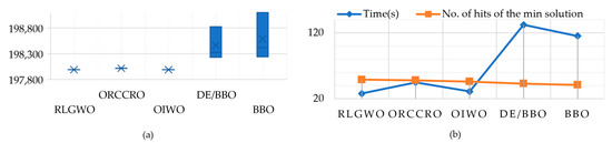
Figure 9.
Results for different methods for the 110-unit system (50 trials): (a) boxplot of the final generation cost; (b) time and number of hits of the minimum solution.
5.1.4. Test System 4
This case study considers 140 generators belonging to Korea’s power system. Twelve generating units possessing a cost function with the valve-point loading effect are utilized, while ramp rate limits, prohibited operating zones and system losses are neglected; the input parameters are available in [14]. The cheapest operating cost obtained using the RLGWO technique is shown in Table 7. The convergence characteristics for 140 generators using GWO and RLGWO methods for the fitness value are presented in Figure 10.
Table 7.
Best simulation results of 140-unit system with loss ( MW).
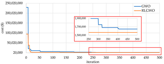
Figure 10.
Comparative convergence characteristic of original GWO and proposed RLGWO algorithm for the 140-unit system.
The statistical results, listed in Table 8, present the maximum, minimum, and average cost obtained by the OIWO method and the proposed RLGWO method over 50 trials. Figure 11 presents a visualization of Table 8. For this test problem, RLGWO produced a lower result than OIWO, as seen in Figure 11a. Compared to OIWO, it found the lowest cost more times out of 50 trials, and was faster than OIWO. This may mean that the increase in problem size affects the RLGWO less than OIWO.
Table 8.
Comparison between different methods taken after 50 trials (140-unit system with loss).
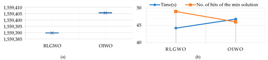
Figure 11.
Results obtaind using different methods for the 140-unit system (50 trials): (a) boxplot of the final generation cost; (b) time and number of hits of the minimum solution.
5.1.5. Test System 5
This case considers a complex system with 160 testing units having multiple options and a valve-point effect. The total load demand is 43,200 MW. The input parameters for 160 generators are generated by multiplying those for the 10-unit system up to reflect a 160-unit system. The data system for 10 generators was taken from [14]. Transmission loss is ignored in this case. The best generating cost obtained by the proposed RLGWO is shown in Table 9. The convergence characteristic of 160 generators with GWO and RLGWO methods for fitness value is presented in Figure 12.
Table 9.
Best simulation results for the 160-unit system with loss ( MW).
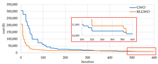
Figure 12.
Comparative convergence characteristic of original GWO and proposed RLGWO algorithm for the 160-unit system.
The maximum, minimum, and average fuel costs acquired by various techniques are represented in Table 10. For this 160-unit system, it can be clearly seen that the proposed algorithm still produced the lowest result (Figure 13a), and the number of times this minimum result was found was the greatest among the algorithms tested (Figure 13b). Furthermore, the RLGWO is still the fastest algorithm of the five algorithms.
Table 10.
Comparison between different methods taken after 50 trials (160-unit system).
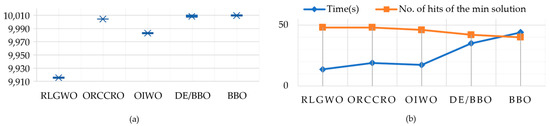
Figure 13.
Results for different methods for the 160-unit system (50 trials): (a) boxplot of the final generation cost; (b) time and number of hits of the minimum solution.
5.2. Comparative Study
5.2.1. Solution Quality
Table 1, Table 3, Table 5, Table 7 and Table 9 present the cheapest generation cost determined by the RLGWO algorithm for five different test systems. It can be clearly seen that the proposed approach usually provides a better solution compared to the results obtained by various most technique. Additionally, the maximum, minimum, and average values acquired using different methods are illustrated in Table 2, Table 4, Table 6, Table 8 and Table 10. These results emphasize the ability of RLGWO to achieve better solutions than most existing techniques.
5.2.2. Computational Efficiency and Robustness
Addressing a large and complex system can increase the time consumption of any algorithm. Therefore, we used execution time to judge the computational efficiency of the optimization technique. The results shown in Table 2, Table 4, Table 6, Table 8 and Table 10, with their corresponding figures, Figure 5, Figure 7, Figure 9, Figure 11 and Figure 13, respectively, prove that the proposed RLGWO requires shorter CPU time to obtain the minimum fuel cost when compared to other reported techniques, except for in the cases of Test 1 and Test 2, where the proposed algorithm ranked second to the least cost. Additionally, those tables and figures also reveal the robustness of the proposed approach. Of the 50 trials performed for the five different test systems, RLGWO obtained the minimum costs 50, 50, 49, 49, and 48 times, respectively. In other words, the efficiency of the RLGWO algorithm for the first two test systems is 100%, and in the remaining cases is 98% or 96%. Additionally, OIWO obtained the minimum cost 47, 46, 46, 46, and 46 times. These results confirm that the performance of RLGWO is outstanding compared to several other methods.
Consequently, the results mentioned above emphasize the ability of RLGWO to obtain high-quality solutions in a way that achieves computational efficiency and robustness.
6. Conclusions and Future Work
This paper presented a newly developed RLGWO algorithm for solving various complex, large-scale economic dispatch problems. To evaluate the feasibility and robustness of the proposed algorithm, five test systems, with 13, 40, 110, 140, and 160 units, respectively, were used. The simulation results revealed the competitive performance of RLGWO when compared to other optimization methods, successfully determining the cheapest generation cost in all cases. GWO is considered a straightforward optimization technique that obviates the need for the initialization of input parameters and has demonstrated its superiority in several optimization problems. The robust tolerance-based adjust searching direction mechanism and opposite-based learning combined with GWO allow it to improve the convergence rate and generate promising search agents. Future work for this research will include applying RLGWO in solving complex real-world power system problems.
Author Contributions
Conceptualization, T.-C.T. and C.-C.L.; methodology, T.-C.T.; software, C.-C.L.; formal analysis, T.-C.T. and C.-C.K.; writing—original draft preparation, T.-C.T.; writing—review and editing, T.-C.T.; visualization, C.-C.L.; supervision, C.-C.K.; All authors have read and agreed to the published version of the manuscript.
Funding
This research received no external funding.
Institutional Review Board Statement
Not applicable.
Informed Consent Statement
Not applicable.
Data Availability Statement
Not applicable.
Acknowledgments
We would like to acknowledge project NSTC112-2622-8-011-011-TE1 for the assistance in our research.
Conflicts of Interest
The authors declare no conflict of interest.
References
- Chakraborty, S.; Senjyu, T.; Yona, A.; Saber, A.; Funabashi, T. Solving economic load dispatch problem with valve-point effects using a hybrid quantum mechanics inspired particle swarm optimisation. IET Gener. Transm. Distrib. 2011, 5, 1042–1052. [Google Scholar] [CrossRef]
- Wood, A.J.; Wollenberg, B.F.; Sheblé, G.B. Power Generation, Operation, and Control, 3rd ed.; Wiley-Interscience: Hoboken, NJ, USA, 2014. [Google Scholar]
- Lee, K.Y.; Park, Y.M.; Ortiz, J.L. Fuel-cost minimisation for both real-and reactive-power dispatches. IEE Proc. C (Gener. Transm. Distrib.) 1984, 131, 85–93. [Google Scholar] [CrossRef]
- Sasson, A.M. Nonlinear Programming Solutions for Load-Flow, Minimum-Loss, and Economic Dispatching Problems. IEEE Trans. Power Appar. Syst. 1969, PAS-88, 399–409. [Google Scholar] [CrossRef]
- Liang, Z.-X.; Glover, J.D. A zoom feature for a dynamic programming solution to economic dispatch including transmission losses. IEEE Trans. Power Syst. 1992, 7, 544–550. [Google Scholar] [CrossRef]
- Wong, K.; Fung, C. Simulated annealing based economic dispatch algorithm. IEE Proc. C Gener. Transm. Distrib. 1993, 140, 509–515. [Google Scholar] [CrossRef]
- Chen, P.-H.; Chang, H.-C. Large-scale economic dispatch by genetic algorithm. IEEE Trans. Power Syst. 1995, 10, 1919–1926. [Google Scholar] [CrossRef]
- Lin, W.-M.; Cheng, F.-S.; Tsay, M.-T. An improved tabu search for economic dispatch with multiple minima. IEEE Trans. Power Syst. 2002, 17, 108–112. [Google Scholar] [CrossRef]
- Ruey-Hsum, L. A neural-based redispatch approach to dynamic generation allocation. IEEE Trans. Power Syst. 1999, 14, 1388–1393. [Google Scholar] [CrossRef]
- Yalcinoz, T.; Short, M.J. Neural networks approach for solving economic dispatch problem with transmission capacity constraints. IEEE Trans. Power Syst. 1998, 13, 307–313. [Google Scholar] [CrossRef]
- Gaing, Z.-L. Particle swarm optimization to solving the economic dispatch considering the generator constraints. IEEE Trans. Power Syst. 2003, 18, 1187–1195. [Google Scholar] [CrossRef]
- Park, J.B.; Shin, J.R.; Lee, K.Y. Closure to discussion of “An improved particle swarm optimization for nonconvex economic dispatch prob-lems”. IEEE Trans. Power Syst. 2010, 25, 2010–2011. [Google Scholar] [CrossRef]
- Bhattacharya, A.; Chattopadhyay, P.K. Biogeography-Based Optimization for Different Economic Load Dispatch Problems. IEEE Trans. Power Syst. 2009, 25, 1064–1077. [Google Scholar] [CrossRef]
- Chiang, C.-L. Improved genetic algorithm for power economic dispatch of units with valve-point effects and multiple fuels. IEEE Trans. Power Syst. 2005, 20, 1690–1699. [Google Scholar] [CrossRef]
- Djokić, S.Ž.; Milanović, J.V.; Rowland, S.M. Advanced voltage sag characterisation II: Point on wave. IET Gener. Trans-Mission. Distrib. 2007, 1, 146–154. [Google Scholar] [CrossRef]
- Noman, N.; Iba, H. Differential evolution for economic load dispatch problems. Electr. Power Syst. Res. 2008, 78, 1322–1331. [Google Scholar] [CrossRef]
- Hou, Y.H.; Wu, W.; Xiong, X. Economic dispatch of power systems based on generalized ant colony optimization method. Zhongguo Dianji Gongcheng Xuebao/Proc. Chin. Soc. Electr. Eng. 2003, 23, 59. [Google Scholar]
- Coelho, L.D.S.; Mariani, V.C. Correction to “Combining of Chaotic Differential Evolution and Quadratic Programming for Economic Dispatch Optimization with Valve-Point Effect”. IEEE Trans. Power Syst. 2006, 21, 1465. [Google Scholar] [CrossRef]
- Vitthaladevuni, P.K.; Alouini, M.S. Discussion of “Economic Load Dispatch-A Comparative Study on Heuristic Optimi-zation Techniques With an Improved Coordinated Aggregation-Based PSO”. IEEE Trans. Broadcast. 2003, 49, 408. [Google Scholar] [CrossRef]
- Meng, K.; Wang, H.G.; Dong, Z.; Wong, K.P. Quantum-Inspired Particle Swarm Optimization for Valve-Point Economic Load Dispatch. IEEE Trans. Power Syst. 2009, 25, 215–222. [Google Scholar] [CrossRef]
- Roy, P.; Roy, P.; Chakrabarti, A. Modified shuffled frog leaping algorithm with genetic algorithm crossover for solving economic load dispatch problem with valve-point effect. Appl. Soft Comput. 2013, 13, 4244–4252. [Google Scholar] [CrossRef]
- Bhattacharya, A.; Chattopadhyay, P.K. Hybrid Differential Evolution With Biogeography-Based Optimization for Solution of Economic Load Dispatch. IEEE Trans. Power Syst. 2010, 25, 1955–1964. [Google Scholar] [CrossRef]
- Dai, C.; Hu, Z.; Su, Q. An adaptive hybrid backtracking search optimization algorithm for dynamic economic dispatch with valve-point effects. Energy 2021, 239, 122461. [Google Scholar] [CrossRef]
- Barisal, A.K.; Prusty, R.C. Large scale economic dispatch of power systems using oppositional invasive weed optimization. Appl. Soft Comput. 2015, 29, 122–137. [Google Scholar] [CrossRef]
- Tizhoosh, H.R. Opposition-Based Learning: A New Scheme for Machine Intelligence. In Proceedings of the International Conference on Com-putational Intelligence for Modelling, Control and Automation and International Conference on Intelligent Agents, Web Technologies and Internet Commerce (CIMCA-IAWTIC’06), Vienna, Austria, 28–30 November 2005. [Google Scholar]
- Mirjalili, S.; Mirjalili, S.M.; Lewis, A. Grey Wolf Optimizer. Adv. Eng. Softw. 2014, 69, 46–61. [Google Scholar] [CrossRef]
- El-Fergany, A.A.; Hasanien, H.H. Single and Multi-objective Optimal Power Flow Using Grey Wolf Optimizer and Dif-ferential Evolution Algorithms. Electr. Power Compon. Syst. 2015, 43, 1548–1559. [Google Scholar] [CrossRef]
- Shakarami, M.R.; Faraji, I. Design of SSSC-based Stabilizer to Damp Inter-Area Oscillations Using Gray Wolf Optimization Algorithm. 2015. Available online: https://sid.ir/paper/907750/en (accessed on 13 February 2023).
- Bhattacharjee, K.; Bhattacharya, A.; Dey, S.H.N. Oppositional Real Coded Chemical Reaction Optimization for different economic dispatch problems. Int. J. Electr. Power Energy Syst. 2014, 55, 378–391. [Google Scholar] [CrossRef]
- Sinha, N.; Chakrabarti, R.; Chattopadhyay, P.K. Evolutionary programming techniques for economic load dispatch. IEEE Trans. Evol. Comput. 2003, 7, 83–94. [Google Scholar] [CrossRef]
- Muro, C.; Escobedo, R.; Spector, L.; Coppinger, R. Wolf-pack (Canis lupus) hunting strategies emerge from simple rules in computational simulations. Behav. Process. 2011, 88, 192–197. [Google Scholar] [CrossRef]
- Long, W.; Jiao, J.; Liang, X.; Tang, M. An exploration-enhanced grey wolf optimizer to solve high-dimensional numerical optimization. Eng. Appl. Artif. Intell. 2018, 68, 63–80. [Google Scholar] [CrossRef]
- Gaidhane, P.J.; Nigam, M.J. A hybrid grey wolf optimizer and artificial bee colony algorithm for enhancing the performance of complex systems. J. Comput. Sci. 2018, 27, 284–302. [Google Scholar] [CrossRef]
- Wang, F.; Zhang, H.; Li, K.; Lin, Z.; Yang, J.; Shen, X.-L. A hybrid particle swarm optimization algorithm using adaptive learning strategy. Inf. Sci. 2018, 436–437, 162–177. [Google Scholar] [CrossRef]
- Shaw, B.; Mukherjee, V.; Ghoshal, S. A novel opposition-based gravitational search algorithm for combined economic and emission dispatch problems of power systems. Int. J. Electr. Power Energy Syst. 2012, 35, 21–33. [Google Scholar] [CrossRef]
- Chatterjee, A.; Ghoshal, S.; Mukherjee, V. Solution of combined economic and emission dispatch problems of power systems by an opposition-based harmony search algorithm. Int. J. Electr. Power Energy Syst. 2012, 39, 9–20. [Google Scholar] [CrossRef]
- Mandal, B.; Roy, P.K. Optimal reactive power dispatch using quasi-oppositional teaching learning based optimization. Int. J. Electr. Power Energy Syst. 2013, 53, 123–134. [Google Scholar] [CrossRef]
- Ergezer, M.; Simon, D. Oppositional biogeography-based optimization for combinatorial problems. In Proceedings of the 2011 IEEE Congress of Evolutionary Computation (CEC), New Orleans, LA, USA, 5–8 June 2011. [Google Scholar]
- Reddy, A.S.; Vaisakh, K. Shuffled differential evolution for large scale economic dispatch. Electr. Power Syst. Res. 2013, 96, 237–245. [Google Scholar] [CrossRef]
- Ciornei, I.; Kyriakides, E. A GA-API Solution for the Economic Dispatch of Generation in Power System Operation. IEEE Trans. Power Syst. 2011, 27, 233–242. [Google Scholar] [CrossRef]
- Orero, S.O.; Irving, M.R. Large scale unit commitment using a hybrid genetic algorithm. Int. J. Electr. Power Energy Syst. 1997, 19, 45–55. [Google Scholar] [CrossRef]
Disclaimer/Publisher’s Note: The statements, opinions and data contained in all publications are solely those of the individual author(s) and contributor(s) and not of MDPI and/or the editor(s). MDPI and/or the editor(s) disclaim responsibility for any injury to people or property resulting from any ideas, methods, instructions or products referred to in the content. |
© 2023 by the authors. Licensee MDPI, Basel, Switzerland. This article is an open access article distributed under the terms and conditions of the Creative Commons Attribution (CC BY) license (https://creativecommons.org/licenses/by/4.0/).