Pixelwise Complex-Valued Neural Network Based on 1D FFT of Hyperspectral Data to Improve Green Pepper Segmentation in Agriculture

Abstract

It seems difficult to recognize an object from its background with similar color using conventional segmentation methods. An efficient way is to utilize hyperspectral images that contain more wave bands and richer information than only RGB components. Particularly in our task, we aim to separate a pepper from densely packed green leaves for automatic picking in agriculture. Given that hyperspectral imaging can be regarded as a kind of wave propagation process, we make a novel attempt of introducing a complex neural network tailored for wave-related problems. Due to the lack of hyperspectral data, pixelwise training is deployed, and 1D fast Fourier transform of the hyperspectral data is used for the construction of complex input. Experimental results have showcased that a complex neural network outperforms a real-valued one in terms of detection accuracy by 3.9% and F1 score by 1.33%. Moreover, it enables the ability to select frequency bands used such as low-frequency components to boost performance as well as prevent overfitting problems for learning more generalization features. Thus, we put forward a lightweight pixelwise complex model for hyperspectral-related problems and provide an efficient way for green pepper automatic picking in agriculture using small datasets.

1. Introduction

Nowadays, the automatic picking of crops is becoming easier due to machine vision and deep learning. However, green peppers differ from most other crops because of their similar color with green leaves as the background. This fact makes it intractable to find them hidden in natural environments. When it is not enough to classify only with the characteristics of the visible wavelengths, the incorporation of hyperspectral imaging to explore more features to be exploited is an effective alternative. One hyperspectral image is a detailed segmentation in the spectral dimension: not only the traditional so-called R, G, B difference but also has various channels in the spectral dimension. Therefore, what is obtained by the hyperspectral device is a data cube, which not only has the information of the image but also expands in the spectral dimension. This results in two merits for hyperspectral imaging. First, it can provide much more clues than a normal RGB camera due to the additional use of invisible wavelengths (generally refers to 700∼1000 nm). Second, a pixel within a hyperspectral image has longer bit depth; thus, numerical diversity will bring greater distinctiveness. As a consequence, hyperspectral imaging has many applications in remote sensing, such as endmember extraction [1] and classification problems [2,3,4] through real-valued neural networks (RVNNs). In this paper, we change another way of thinking to tackle this problem by regarding hyperspectral imaging as a kind of wave propagation process and utilizing complex-valued neural networks (CVNNs) instead that work better with wave-related problems [5,6].

CVNN is first put forward on the basis of phase and amplitude concepts. This property makes it compatible and easier to deal with wave-related signals or the waves themselves (electromagnetic waves, sound waves, and ultrasonic waves). As a physical fact, amplitude corresponds to wave energy, while phase difference represents the time process or change of position. This wave-oriented advantage can be widely used in general signal processing with Fourier synthesis or frequency domain processing via Fourier transform. To this end, we use Fourier transform to build complex input as a powerful mathematical tool to make it more physically reasonable. Analogously, a recent study also combines Fourier transform and CVNN for hyperspectral single-image super resolution [7]. On the other hand, weight multiplication at synapses produces phase rotation and amplitude decay (or amplification), which reduces noneffective degrees of freedom during the learning process, thereby enhancing generalization properties compared to 2D RVNNs. In light of the above two reasons, employing a complex neural network is possibly more suitable as a viable alternative. Our contributions can be summarized as follows:

• We propose a lightweight pixelwise complex-valued neural network (CVNN) assisted by 1D Fourier transform to address hyperspectral classification problems.
• We provide an efficient way for green pepper automatic picking in agriculture using small datasets.

2. Related Work

2.1. Green Pepper Automatic Picking

In order to reduce labor intensity and time cost, whether green peppers can be accurately identified by picking robots has become an urgent problem. Since the shape and size information of crops is of greater importance to help robot hands fit the pepper and find stems to be cut, segmentation methods have become the mainstream due to their ability to emphasize the precise shape of green peppers. There are many approaches to segmenting a pepper from its leaves. For example, Eizentals et al. [8] study green peppers on HSV color space that are closer to a human’s perceptual experience of color, while Hespeler et al. [9] introduce thermal imaging into deep learning for green pepper detection. Alternatively, hyperspectral imaging has become a powerful tool because of its extra features hidden in invisible wavelengths, especially when the available visual cues cannot provide sufficient information. In collaboration with hyperspectral imaging, many classical methods have been proposed such as Support Vector Machine (SVM) [10], Convolutional Neural Network (CNN) [11], and 3D neural network [12]. From a different angle, another recent novel study [13] enables the design of an optical filter to select useful bands rather than design network structures. As a result, all these methods are realized with RVNNs whereas CVNNs are rarely seen in previous related works.

2.2. Complex-Valued Neural Network (CVNN)

Up until now, the great majority of deep learning building blocks and network architectures are achieved by real-valued representations and operations. However, CVNN has proved its superiority in terms of rich representation capacity [14], easier optimization [15], fast learning [16] and better generalization properties [17]. There are many application systems employing CVNNs, for example, Principal Component Analysis (PCA)-based blind source separation in Sonar [18], ultrasonic fault detection [19], fuzzy compensation image processing [20], etc. Despite bringing about entirely new neural architectures, CVNN has been marginalized because of the lack of building modules required to design such networks. Accordingly, a set of unified modules and components, including linear layer, ReLU activation function, convolutional layer, and Batch Normalization under the complex version have been proposed [21,22]. Owing to these two works, CVNN is successfully applied to computer vision tasks such as image classification on CIFAR-10 and automatic music transcription on MusicNet. As our previous work [23], we introduce CVNN to hyperspectral imaging problems, whereas the methods of making complex input are less reasonable by folding in half in the spectral dimension. To this end, we try to use Fourier transform at this time instead as a real-to-complex converter so that the amplitude and phase of the complex numbers will be given real physical meanings. As can be seen later, this method can also control the frequency bands fed to the complex neural network for performance enhancement.

3. Method

3.1. Dataset and Pre-Processing

Due to the lack of a public dataset of green peppers, we have to use our hyperspectral camera (NH-2 by EBA JAPAN CO., LTD., Tokyo, Japan) to capture 20 images (subject to time cost) in the greenhouse, each of which is of size 480 × 640 and has 121 channels ranging from 400∼1000 nm with an interval of 5 nm.

Since the hyperspectral image has various wave bands, it is prone to suffer from light influence if the source of illumination for each wavelength is not even. However, this light inhomogeneity is band-oriented but works the same on two different objects in the same scene. Therefore, if we also take a photo of the white board using the same hyperspectral camera, the light influence can be removed by division operation between them. That is why we place a white reflectance standard in the scene in advance. This method is called “white and dark correction” which is efficient for hyperspectral data pre-processing [24,25], and we give a simple illustration in the above section of Figure 1.

However, 20 images after pre-processing are not enough to train such a deep learning model. Motivated by [26], we deploy pixelwise training, and accordingly, one hyperspectral image with size 480 × 640 has 0.3 million pixels available for training. To make an intuitive explanation of how we construct our manual dataset, a process display is drawn in the below section of Figure 1. First, the RGB image regarding the hyperspectral image is acquired through the RGB response table. Second, we pick distinguishable pixel samples on eye-friendly RGB images and obtain their corresponding spectral vectors in the data cube by position mapping. For convenience in later comparison experiments, we discard the last dimension that has little influence. Last but not least, a binary label is added (1 or 0) by human eye supervision to complete the making of a training sample.

3.2. Discrete Fourier Transform

The algorithm that transforms sampled data in the time domain into the frequency domain is called discrete Fourier transform (DFT). DFT connects the time domain and frequency domain of the sampled signal such that the phase and amplitude information can be easily analyzed. We use 1D-DFT here since our training data are a set of spectral vectors. Let $\mathit{x}={(x_0,x_1,\cdots ,x_{119})}^T$ be one of our training samples; its 1D-DFT is still the same number of samples but in the frequency domain representation, namely $DFT\left[\mathit{x}\right]=\mathit{X}={\left\{X_k\right\}}_{k=0}^{119}$. The relationship between them can be formulated as follows:

$$X_k=\sum _{n=0}^{119}{x}_n{e}^{-j2\pi kn/120}(k=0,1,\cdots ,119)$$

(1)

By separating cosine and sine components as real and imaginary parts, respectively, each sample $\mathit{x}$ is transformed into complex numbers to enable the training of the complex neural network. For inference needs, this process is handed over to the fast Fourier transform (FFT) algorithm in particular applications.

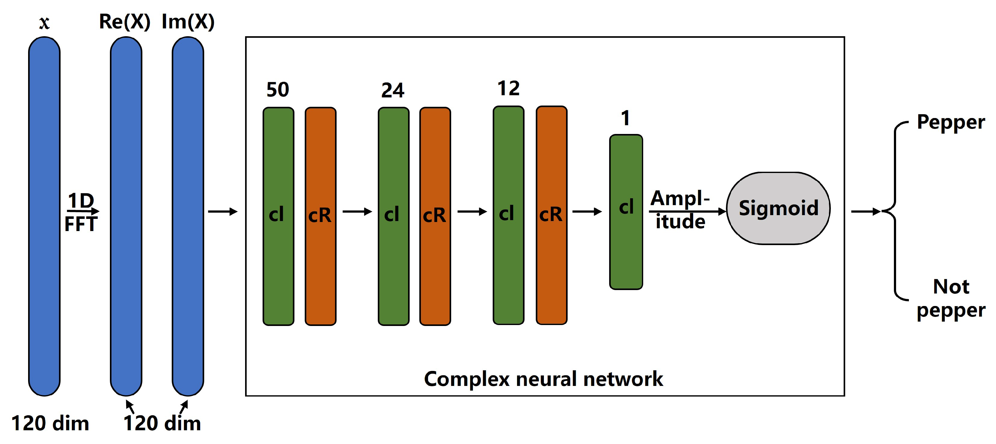
3.3. Complex Neural Network

In order to build a complex neural network, it is necessary to introduce its basic components: linear layer and ReLU activation function under the complex version which we use in this paper.

Considering a simple example, where it only contains a single layer with two input nodes and two output nodes (for real-valued situations). For convenience, we assume that there is no bias and the activation function is identical mapping. Let $X_{in}=(X_{i{n}_1},X_{i{n}_2})$ be input and $X_{out}=(X_{ou{t}_1},X_{ou{t}_2})$ be output; then, this linear layer mapping can be written as follows:

$$\left[\begin{array}{c}{X}_{ou{t}_1}\\ X_{ou{t}_2}\end{array}\right]=\left[\begin{array}{cc}a& b\\ c& d\end{array}\right]\left[\begin{array}{c}{X}_{i{n}_1}\\ X_{i{n}_2}\end{array}\right]$$

(2)

where $a,b,c,d$ are independent training parameters. Since this is an ill-posed problem, we can obtain various possible mappings through learning. In contrast, when considering complex-valued situations, $X_{in}$ and $X_{out}$ will be both regarded as complex numbers (real number pairs); thus, input and output nodes will degenerate to only one. Decomposing the real and complex part, this mapping of one complex number to another is formulated as:

$$\left[\begin{array}{c}{X}_{ou{t}_1}\\ X_{ou{t}_2}\end{array}\right]=\left[\begin{array}{cc}\left|\omega \right|cos\theta & -\left|\omega \right|sin\theta \\ \left|\omega \right|sin\theta & \left|\omega \right|cos\theta \end{array}\right]\left[\begin{array}{c}{X}_{i{n}_1}\\ X_{i{n}_2}\end{array}\right]$$

(3)

where $\left|\omega \right|$ and $\theta$ = arg($\omega$) denote amplitude decay (or amplification) and phase rotation, respectively. As a result, degrees of freedom could reduce because links between parameters are established through phase and amplitude. In general, the substantial advantage of neural networks lies in learning the high degrees of freedom. However, supposing that we know a priori that the learning target includes phase and amplitude, more meaningful generalization features can be obtained by utilizing a complex neural network to reduce the potentially harmful part of the degrees of freedom.

As for the complex ReLU activation function, it is relatively straightforward to understand. By applying respective ReLUs on both the real and complex parts of a neuron z, we can obtain the expression of cReLU:

$$cReLU\left(z\right)=ReLU\left(R\right(z\left)\right)+jReLU\left(I\right(z\left)\right)$$

(4)

3.4. The Whole Pipeline

The whole pipeline of our algorithm is presented in Figure 2. As can be seen, a spectral vector with 120 channels as hyperspectral input is translated into complex numbers by 1D fast Fourier transform (1D-FFT), which is followed by a small complex neural network to predict whether it belongs to pepper or not. In particular, we use 3 intermediate complex linear layers with 50, 24, and 12 neural nodes, respectively, and an output complex linear layer. As for intermediate layers, a complex ReLU activation function follows closely for each of them. To obtain the final real-valued binary prediction, we calculate the amplitude of the output and feed it into a sigmoid function.

4. Experiments

4.1. Training Details

Twenty images are divided into two parts, and 8 images are used for picking pixelwise training samples, as mentioned in Figure 1 while the remaining 12 are used for testing. As a result, 56,967 positive samples (peppers) and 63,478 negative samples (non-peppers) are selected to make the training dataset. During the training process, the training epoch and batch size are set to 10 and 64, respectively. We adopt Adam as an optimizer and binary cross-entropy as a loss function. All the experiments are conducted with the PyTorch framework on NVIDIA Geforce GTX 1080Ti GPU.

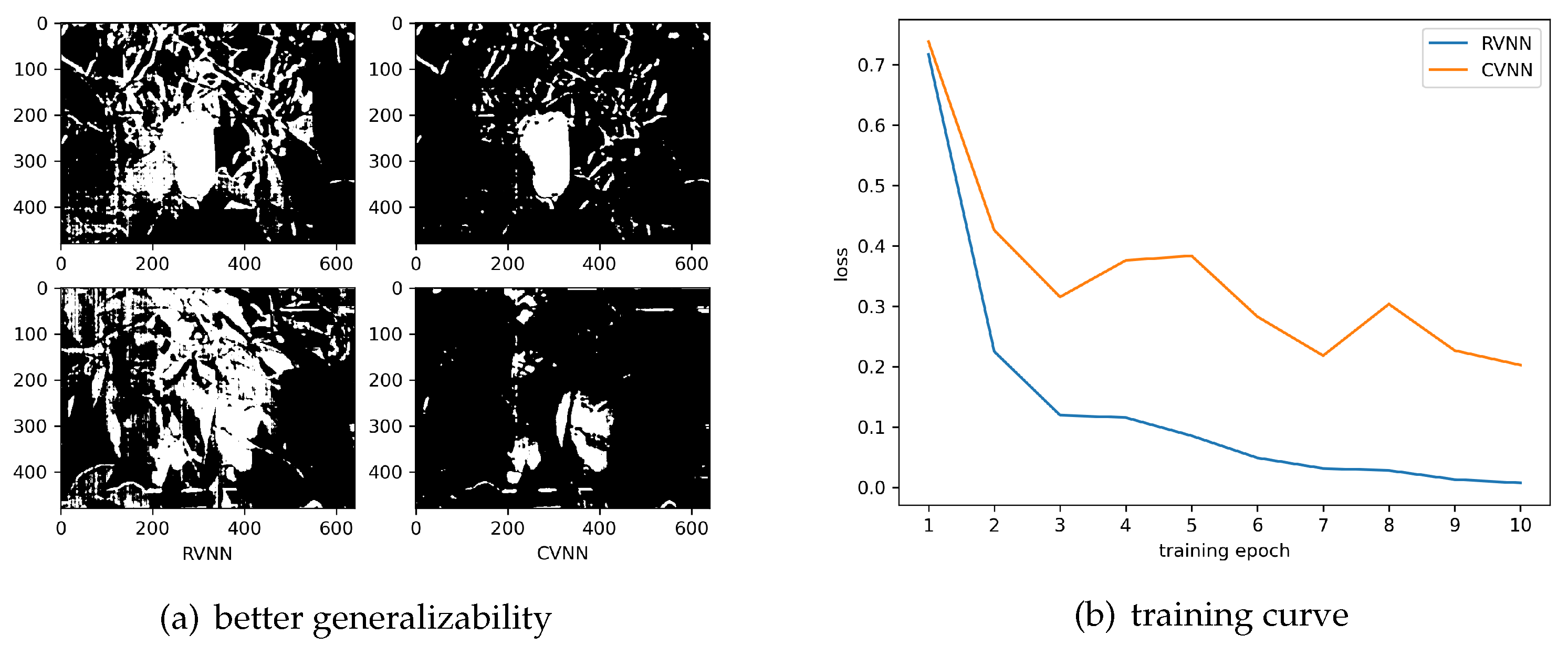
4.2. Real vs. Complex

To demonstrate the effectiveness of the incorporation of CVNN, we illustrate our qualitative and quantitative results in Figure 3 and

Table 1. Quantitative comparison results between different models in terms of accuracy, recall rate and F1 score. The best and poorest performance for each metric is marked as pink and light gray signs, respectively.

	Accuracy	Recall Rate	F1 Score
RVNN	90.99%	83.21%	86.92%
CVNN	94.89%	82.48%	88.25%
CVNN ($X_{0\sim 60}$)	94.49%	82.97%	88.36%
CVNN ($X_{0\sim 30}$)	93.71%	85.73%	89.55%
CVNN ($X_{31\sim 60}$)	72.75%	64.83%	68.56%

, respectively. Given that finding peppers as much as possible is of the same importance under the premise of accurate classification, we report three kinds of metrics including accuracy, recall rate, and F1 score for a comprehensive evaluation of the experimental results. For fairness, RVNN as a comparison is trained under the same configuration, including the network structure described in Figure 2 and training details in Section 4.1. As can be seen in the 3rd and 4th columns in Figure 3, CVNN has higher accuracy than a real-valued one at the cost of sacrificing a bit of recall rate. However, we only need a non-low recall rate to determine the general position and shape of the green pepper to help the robot hands locate the stems to be cut; thus, a small part of the missing recall rate can be made up after this pepper is picked. In contrast, more accurate classification of hard negative samples helps to avoid unnecessary time wasted on the wrong location. This fact can also be proved by specific numbers in the first two rows in Table 1, where CVNN outperforms RVNN by 3.9% and 1.33% in terms of accuracy and F1 score, respectively, despite a 0.73% drop in recall rate.

4.3. Half of Frequencies vs. Quarter of Frequencies

CVNN excels a real-valued one but inevitably doubles the training parameters due to the extra complex part. However, since the input signal is a real value, only half of the frequencies have the meaning, and no additional information is carried by the other half because of conjugate symmetry. That is to say, $X_k=X_{120-k}^{*}$ as for FFT results ${\left\{X_k\right\}}_{k=0}^{119}$ except for direct-current (DC) component $X_0$ and symmetry axis $X_{60}$. To this end, we use only half of frequencies $X_0\sim X_{60}$, which is enough to represent the whole information of the frequency domain. As can be seen in Figure 3 and Table 1, there is not a great deal of difference between them, which indicates that the additional training parameters introduced by the complex part can be reduced for real input.

Additionally, we make another attempt to further narrow the frequency range by only using low-frequency components of FFT results. Since we do not conduct a frequency shift (FFTshift), the low-frequency components lie on the far left ($X_0\sim X_{30}$) and far right ($X_{90}\sim X_{119}$) of the frequency band, and we choose the former as explained before. As a result in the second last column and row in Figure 3 and Table 1, we surprisingly find that a further reduction of parameters does not bring about a drop in performance; conversely, it outperforms the results from using half of the frequencies and full frequencies by 2.94% and 1.19% in terms of recall rate and F1 score despite a 0.78% loss in accuracy. It may be attributed to the fact that neural networks prefer low-frequency components while selectively ignoring high-frequency ones; thus, pure low-frequency input without interference from noise in high-frequency components will lead to better outcomes. To make it more convincing, we also conduct comparison experiments by using pure high-frequency components ($X_{31}\sim X_{60}$). As might have been expected, it turns out to be a mess with much noise reflected on qualitative results in the last column in Figure 3. We can also clearly see from the last two rows in Table 1 that it has the poorest performance on all metrics, which again proves that the low-frequency part plays a leading role in the training of the neural network whereas the high-frequency part will disturb it.

4.4. Overfitting Problem

The ability to alleviate the overfitting problem of CVNN has been discussed earlier, and this section will give an explanation in detail. Figure 4b illustrates two training curves of RVNN and CVNN, respectively, in which the loss of RVNN decreases monotonically until convergence as the epoch grows, whereas CVNN endures a higher loss with an unsteady learning process. However, CVNN learns a better generalization feature in spite of the difficulty of training, which can be demonstrated by the qualitative results on two hard samples within the testing set. As shown in Figure 4a, when peppers are surrounded by dense green leaves, CVNN still enables an acceptable location, while one could not recognize where peppers are at the first glance of the results from RVNN. This is because RVNN has a high degrees of freedom, so it tends to choose features that cater to the training dataset as much as possible but may not fit on the testing dataset. From this perspective, CVNN shows its huge advantage in preventing overfitting.

5. Conclusions

Green pepper automatic picking is an intractable problem in agriculture because it is hard to distinguish a pepper from densely packed green leaves with similar colors by the naked eye as well as picking robots. To find more features helpful for classification, we decide to incorporate hyperspectral imaging so that richer information hidden in invisible wavelengths can also be leveraged. Since hyperspectral imaging can be regarded as a kind of wave propagation process, we introduce a complex neural network that is good at dealing with wave-related problems. Given that hyperspectral images are expensive to obtain, we decide to deploy pixelwise training and use 1D fast Fourier transform of the hyperspectral data for the construction of complex input. A complex neural network excels a real-valued one in three aspects. First, it promotes detection accuracy to a great extent, which is important for the fast and accurate location of green peppers. Second, it can selectively control the range of frequency bands used assisted by Fourier transform to bring an overall performance boost as well as reduce the training parameters. Last but not least, it enables the ability to prevent overfitting problems caused by high degrees of freedom; thus, more generalization features can be learned. Supported by both qualitative and quantitative results, this pixelwise complex model does work and tends to be easier to realize in practical applications with only small datasets. As a consequence, we have proposed an efficient method for the robotic harvesting of green peppers in agriculture and bring the application of complex neural networks to a new field.

References

1. Fu, Z.; Pun, C.-M.; Gao, H.; Lu, H. Endmember extraction of hyperspectral remote sensing images based on an improved discrete artificial bee colony algorithm and genetic algorithm. Mob. Netw. Appl. 2018, 25, 1033–1041. [Google Scholar] [CrossRef]
2. Chen, Y.; Jiang, H.; Li, C.; Jia, X.; Ghamisi, P. Deep Feature Extraction and Classification of Hyperspectral Images Based on Convolutional Neural Networks. IEEE Trans. Geosci. Remote Sens. 2016, 54, 6232–6251. [Google Scholar] [CrossRef] [Green Version]
3. Xie, C.; Yang, C.; He, Y. Hyperspectral imaging for classification of healthy and gray mold diseased tomato leaves with different infection severities. Comput. Electron. Agric. 2017, 135, 154–162. [Google Scholar] [CrossRef]
4. Ishida, T.; Kurihara, J.; Viray, F.A.; Namuco, S.B.; Paringit, E.C.; Perez, G.J.; Takahashi, Y.; Marciano, J.J., Jr. Tetsuro Ishida, Junichi Kurihara, Fra Angelico Viray, et.al. A novel approach for vegetation classification using UAV-based hyperspectral imaging. Comput. Electron. Agric. 2018, 144, 80–85. [Google Scholar] [CrossRef]
5. Hiros, A. Complex-valued neural networks. Stud. Comput. Intell. 2006, 32, 1–160. [Google Scholar]
6. Hirose, A. Complex-valued neural networks: The merits and their origins. In Proceedings of the International Joint Conference on Neural Networks, Atlanta, GA, USA, 14–19 June 2009. [Google Scholar]
7. Aburaed, N.; Alkhatib, M.Q.; Marshall, S.; Zabalza, J.; Al Ahmad, H. Complex-valued neural networks for hyperspectral single image super resolution. Photonex 2023, 12338, 102–109. [Google Scholar]
8. Eizentals, P.; Oka, K. 3D pose estimation of green pepper fruit for automated harvesting. Comput. Electron. Agric. 2016, 128, 127–140. [Google Scholar] [CrossRef]
9. Hespeler, S.C.; Nemati, H.; Dehghan-Niri, E. Non-destructive thermal imaging for object detection via advanced deep learning for robotic inspection and harvesting of chili peppers. Artif. Intell. Agric. 2021, 5, 102–117. [Google Scholar] [CrossRef]
10. Melgani, F.; Bruzzone, L. Classification of hyperspectral remote sensing images with support vector machines. IEEE Trans. Geosci. Remote Sens. 2004, 42, 1778–1790. [Google Scholar] [CrossRef] [Green Version]
11. Hu, W.; Huang, Y.; Li, W.; Fan, Z.; Li, H. Deep Convolutional Neural Networks for Hyperspectral Image Classification. J. Sens. 2015, 2015, 258619. [Google Scholar] [CrossRef] [Green Version]
12. Shi, C.; Pun, C.-M. Superpixel-based 3D deep neural networks for hyperspectral image classification. Pattern Recognit. 2018, 74, 600–616. [Google Scholar] [CrossRef]
13. Yu, J.; Kurihara, T.; Zhan, S. Optical Filter Net: A Spectral-Aware RGB Camera Framework for Effective Green Pepper Segmentation. IEEE Access 2021, 9, 90142–90152. [Google Scholar] [CrossRef]
14. Wisdom, S.; Powers, T.; Hershey, J.; Le Roux, J.; Atlas, L. Full-capacity unitary recurrent neural networks. Adv. Neural Inf. Process. Syst. 2016, 29, 4880–4888. [Google Scholar]
15. Nitta, T. On the critical points of the complex-valued neural network. In Proceedings of the 9th International Conference on Neural Information Processing, Penang, Malaysia, 19–21 December 2002; Volume 3, pp. 1009–1103. [Google Scholar]
16. Arjovsky, M.; Shah, A.; Bengio, Y. Unitary evolution recurrent neural networks. In Proceedings of the International Conference on Machine Learning (ICML), New York, NY, USA, 19–24 June 2016; pp. 1120–1128. [Google Scholar]
17. Hirose, A.; Yoshida, S. Generalization Characteristics of Complex-Valued Feedforward Neural Networks in Relation to Signal Coherence. IEEE Trans. Neural Netw. Learn. Syst. 2012, 23, 541–551. [Google Scholar] [CrossRef] [PubMed]
18. Zhang, Y.; Ma, Y. CGHA for principal component extraction in the complex domain. IEEE Trans. Neural Netw. 1997, 85, 1031–1036. [Google Scholar] [CrossRef] [PubMed] [Green Version]
19. Birx, D.L.; Pipenberg, S.J. A complex mapping network for phase sensitive classification. IEEE Trans. Neural Netw. 1993, 41, 127–135. [Google Scholar] [CrossRef] [PubMed]
20. Aizenberg, I.N.; Paliy, D.; Zurada, J.M.; Astola, J. Blur Identification by Multilayer Neural Network Based on Multivalued Neurons. IEEE Trans. Neural Netw. 2008, 19, 883–898. [Google Scholar] [CrossRef]
21. Trabelsi, C.; Bilaniuk, O.; Zhang, Y. Deep Complex Networks. In Proceedings of the 6th International Conference on Learning Representations (ICLR), Vancouver, BC, Canada, 30 April–3 May 2016. [Google Scholar]
22. Guberman, N. On complex valued convolutional neural networks. arXiv 2016, arXiv:1602.09046. [Google Scholar]
23. Liu, X.; Yu, J.; Kurihara, T.; Xu, L.; Niu, Z.; Zhan, S. Hyperspectral imaging for green pepper segmentation using a complex-valued neural network. Optik 2022, 265, 169527. [Google Scholar] [CrossRef]
24. Zhang, Y.M.; Wang, P.; Bai, J.R.; Dong-Ya, M.A. Establishment of Identification and Classification Model of PE, PP and PET Based on Near Infrared Spectroscopy; Modern Chemical Industry: Mumbai, India, 2016. [Google Scholar]
25. Guo, Z.; Zhao, C.; Huang, W.; Peng, Y.; Li, J.; Wang, Q. Intensity correction of visualized prediction for sugar content in apple using hyperspectral imaging. Trans. Chin. Soc. Agric. Mach. 2015, 46, 227–232. [Google Scholar]
26. Bac, C.W.; Hemming, J.; van Henten, E.J. Robust pixel-based classification of obstacles for robotic harvesting of sweet-pepper. Comput. Electron. Agric. 2013, 96, 148–162. [Google Scholar] [CrossRef]
Figure 1. Data pre-processing and making process. Different color arrows on the spectrum represent different light intensities for each wavelength. RRT is short for RGB response table.
Applsci 13 02697 g001
Figure 2. The whole pipeline of our proposed complex model. “cl” and “cR” represent the abbreviation for the complex linear layer and complex ReLU activation function, respectively, and the number on each complex linear layer denotes its number of complex neural nodes.
Applsci 13 02697 g002
Figure 3. Comparison results between RVNN and CVNN as well as several variations for CVNN. X 0 60 , X 0 30 and X 31 60 represent the only use of the first half, first quarter (low-frequency) and second quarter (high-frequency) of frequency components, respectively.
Applsci 13 02697 g003
Figure 4. (a) shows that CVNN can learn better generalization characteristics of the data to prevent overfitting, and (b) reflects this fact by training curves.
Applsci 13 02697 g004