Figure 1.
Proposed MSE feature fusion architecture. It consists of the following stages: data inputs, feature extraction, merging-squeeze-excitation feature fusion, and classification. The inputs are the sensor data from N IMUs attached to several parts of the user body. Each branch extracts a set of feature maps independently by using a 1D CNN model. In the merging-squeeze-excitation feature fusion stage, each set of feature maps is calibrated by using a set of channel weights. A merging method combines the sets of channel-weighted feature maps and produces a new set of channel-weighted and merged feature maps , which is used later in the classification process.
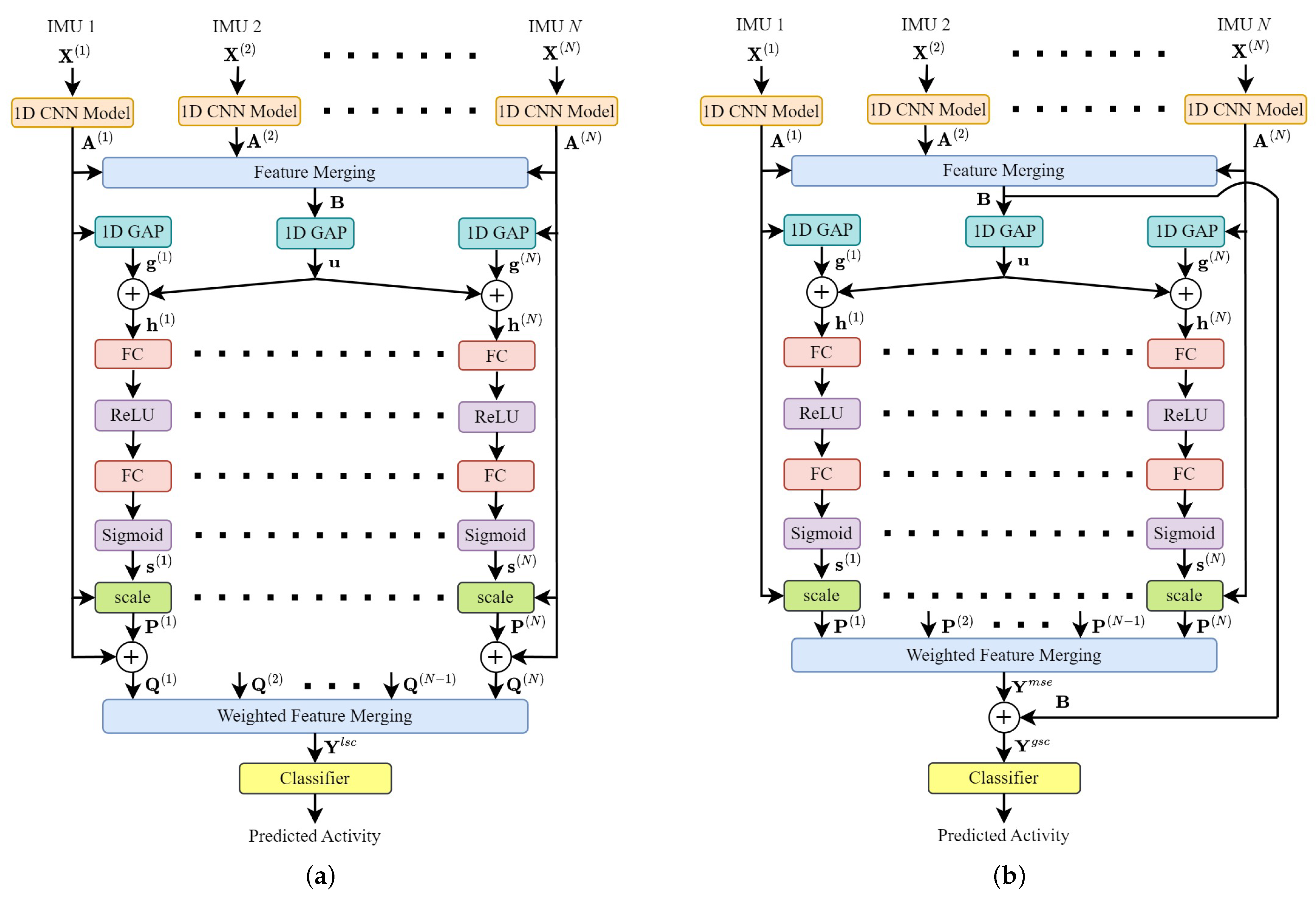
Figure 2.
MSE feature fusion architectures with skip connections. There are two types: (a) MSE feature fusion with local skip connections. A skip connection is added to each branch. As a result, we combine the feature maps instead of . The output still contains the feature maps directly obtained from 1D CNN models and (b) MSE feature fusion with a global skip connection. The pre-merged feature maps are added to the feature maps . As a result, the output feature maps contain both pre-merged feature maps (no channels weighted) and channel-weighted feature maps.
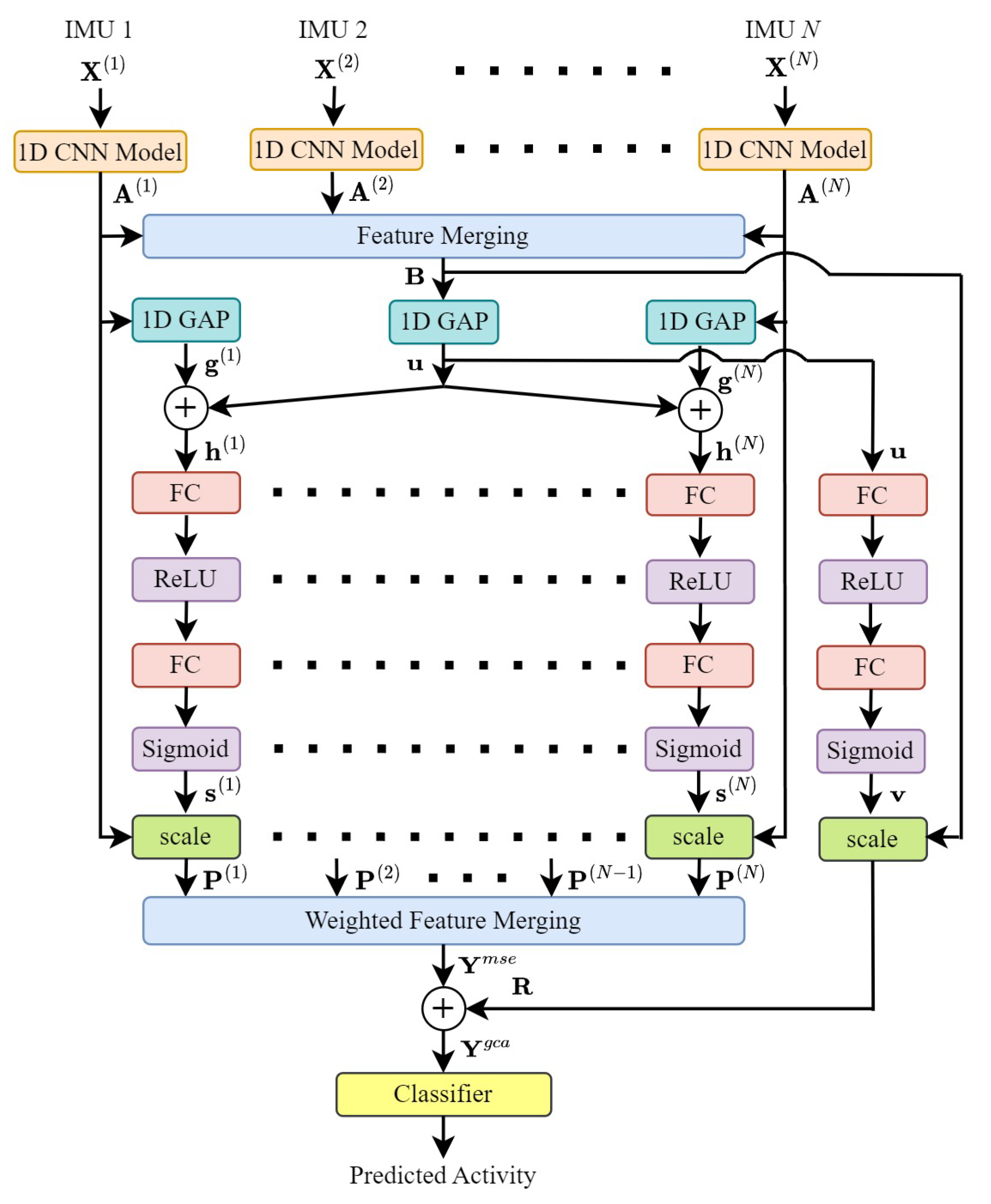
Figure 3.
MSE feature fusion architecture with global channel attention. We compute an additional set of channel-weighted feature maps which is obtained from the pre-merged feature maps . The output feature maps contain both (where feature maps are calibrated and, then, merged) and (where feature maps are merged and, then, calibrated).
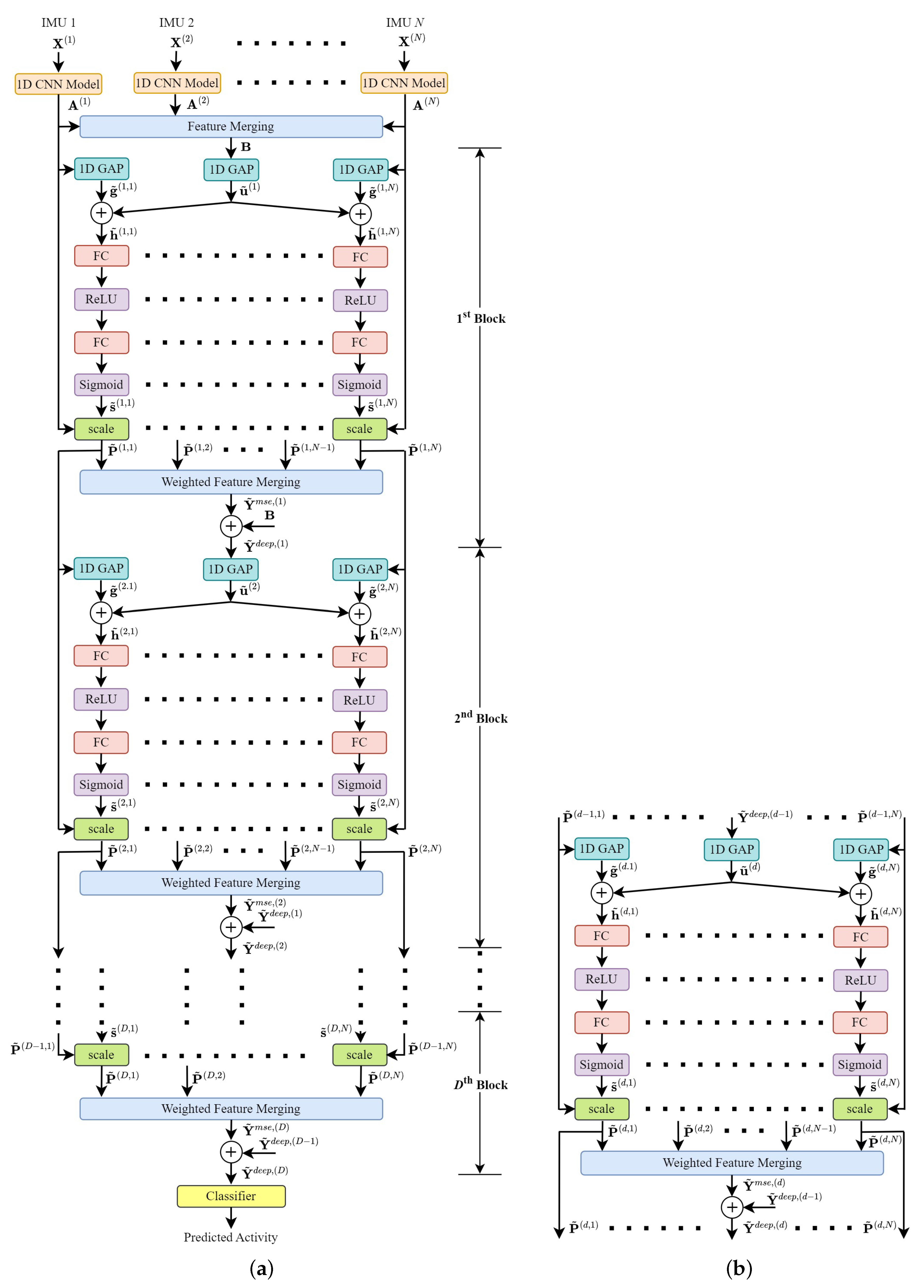
Figure 4.
Deep MSE feature fusion. We implement a series of D MSE feature fusion blocks such that the feature maps , , …, are calibrated and merged several times as shown in (a) deep MSE feature fusion architecture, where the structure of the d-th MSE feature fusion block is shown in (b). The output feature maps are used in the classification process.
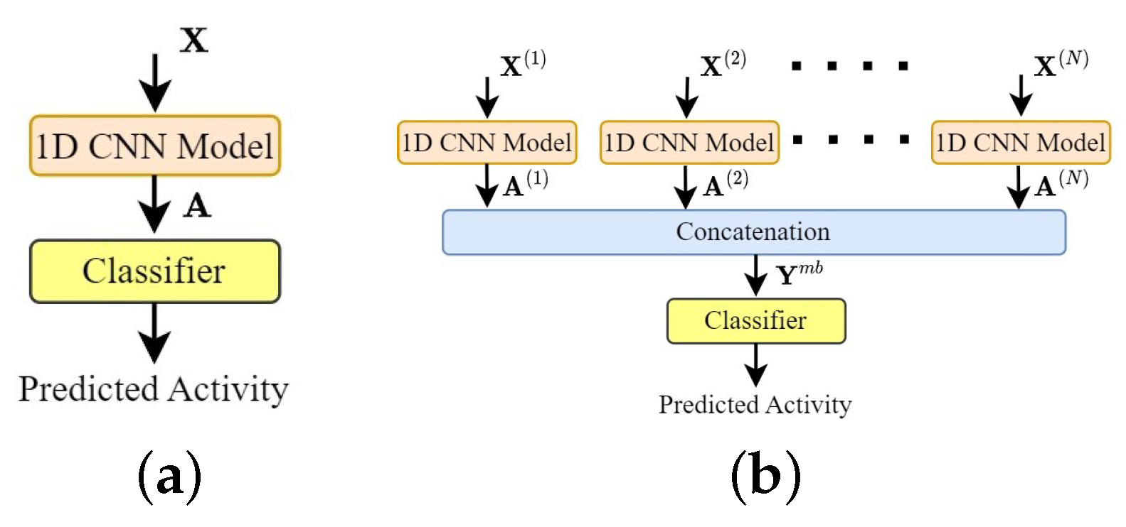
Figure 5.
Baseline architectures. (a) Single-branch architecture. (b) Multi-branch architecture.
Figure 5.
Baseline architectures. (a) Single-branch architecture. (b) Multi-branch architecture.
| Symbol | Definition |
|---|
| A vector of channel-wise statistics according to the local feature maps at the n-th branch. |
| A vector of channel-wise statistics according to the addition of and at the n-th branch. |
| A vector of channel weights for the local feature maps at the n-th branch. |
| A vector of channel-wise statistics according to the pre-merged feature maps . |
| A vector of channel weights for the pre-merged feature maps . |
| A 3D array of local feature maps at the n-th branch. |
| A 3D array of pre-merged feature maps. |
| A 3D array of channel-weighted feature maps according to the local feature maps at the n-th branch. |
| A 3D array of channel-weighted feature maps according to the addition of and at the n-th branch. |
| A 3D array of channel-weighted feature maps according to the pre-merged feature maps . |
| A 3D array of sensor data at the n-th branch (obtained from the n-th IMU). |
| A 3D array of channel-weighted and merged feature maps, which is the output of the MSE feature |
| | fusion with global channel attention. |
| A 3D array of channel-weighted and merged feature maps, which is the output of the MSE feature |
| | fusion with a global skip connection. |
| A 3D array of channel-weighted and merged feature maps, which is the output of the MSE feature fusion with local skip connections. |
| A 3D array of channel-weighted and merged feature maps, which is the output of the MSE feature fusion. |
| Symbol | Definition |
|---|
| A vector of channel-wise statistics according to the feature maps at the n-th branch in the d-th MSE feature fusion block. |
| A vector of channel-wise statistics according to the addition of and at the n-th branch in the d-th MSE feature fusion block. |
| A vector of channel weights for the feature maps at the n-th branch in the d-th MSE feature fusion block. |
| A vector of channel-wise statistics according to the merged and channel-weighted feature maps in the d-th MSE feature fusion block. |
| A 3D array of local feature maps at the n-th branch. |
| A 3D array of pre-merged feature maps. |
| A 3D array of channel-weighted feature maps according to the feature maps at the n-th branch in the d-th MSE feature fusion block. |
| A 3D array of sensor data at the n-th branch (obtained from the n-th IMU). |
| A 3D array of channel-weighted and merged feature maps, which is the output of the weighted feature merging in the d-th MSE feature fusion block. |
| A 3D array of channel-weighted and merged feature maps, which is the output of the d-th MSE feature fusion. |
Table 3.
A summary of DL models with SE blocks for HAR using sensor data.
Table 3.
A summary of DL models with SE blocks for HAR using sensor data.
| Year | Ref. | Dataset | Device | DL Model |
|---|
| 2021 | [21] | UCI HAR, WISDM | Smartphone | CNN with an SE block |
| 2022 | [17] | HASC, UCI HAR, WISDM | Smartphone | State-of-the-art CNNs
with SE blocks |
| 2022 | [18] | HAPT, MobiAct v2.0 | Smartphone | CNN with a residual block,
an SE block, and BiGRU |
Table 4.
A summary of multi-branch DL architectures for HAR using sensor data.
Table 4.
A summary of multi-branch DL architectures for HAR using sensor data.
| Year | Ref. | Dataset | Device | Category | DL Model | Feature Fusion |
|---|
| 2018 | [19] | Opportunity, Order Picking, PAMAP2 | IMUs | Multiple Inputs | CNN | Concatenation |
| 2019 | [20] | UCI HAR, WISDM | Smartphone | Multiple DL Models | CNN | Concatenation |
| 2020 | [22] | DG, DSAD, PAMAP2, RealWorld-HAR | IMUs | Multiple Inputs | CNN | Concatenation |
| 2020 | [24] | WISDM | Smartphone | Multiple DL Models | CNN | Concatenation |
| 2020 | [25] | MHEALTH, WISDM | IMUs, Smartphone | Multiple DL Models | CNN and LSTM | Concatenation |
| 2021 | [21] | UCI HAR, WISDM | Smartphone | Multiple DL Models | CNN with an SE block | Concatenation |
| 2021 | [26] | PAMAP2, UCI HAR, WISDM | IMUs, Smartphone | Multiple DL Models | CNN and GRU | Concatenation |
| 2021 | [27] | Self-Recorded Data, UCI HAR | IMUs, Smartphone | Multiple DL Models | CNN | Concatenation |
| 2022 | [28] | PAMAP2, UCI HAR, WISDM | IMUs, Smartphone | Multiple DL Models | CNN | Concatenation |
| 2023 | [23] | Opportunity, PAMAP2, UniMiB-SHAR | IMUs, Smartphone | Multiple Inputs | CNN and Residual Blocks | Concatenation |
Table 5.
A summary of related SE fusion.
Table 5.
A summary of related SE fusion.
| Year | Ref. | Modality | Dataset | Classification | Fusion Mechanism |
|---|
| 2021 | [29] | EEG | BCI IV 2a, HGD | Motor imagery tasks | SE mechanism |
| 2022 | [34] | EEG, EOG | MASS-SS3 | Sleep staging | Multimodal SE mechanism |
| 2022 | [35] | RGB videos, | ETRI-Activity3D | Elderly activities | Expansion SE mechanism skeleton sequences |
Table 6.
A summary of sensor data from three datasets.
Table 6.
A summary of sensor data from three datasets.
| | PAMAP2 | DaLiAc | DSAD |
|---|
| Sensor | 2 accelerometers, 1 gyroscope, 1 magnetometer | 1 accelerometer, 1 gyroscope | 1 accelerometer, 1 gyroscope, 1 magnetometer |
| Sampling Rate | 100 Hz | 200 Hz | 25 Hz |
| No. IMUs (N) | 3 | 4 | 5 |
| Positions | wrist, chest, ankle | right wrist, chest, right hip, left ankle | torso, right arm, left arm, right leg, left leg |
| No. Sensor Data Types | 12 | 6 | 9 |
| per IMU (M) | | | |
| No. Subjects | 9 | 19 | 8 |
| No. Activities | 12 | 13 | 19 |
| Window Size | 3 s | 3 s | 5 s |
| Segment Length (L) | 300 data points | 600 data points | 125 data points |
| No. Segments | 5764 | 7802 | 9120 |
Table 7.
The width W and the number of channel C of the feature maps obtained from LeNet5, AlexNet, and VGG16 by using the PAMAP2, DaLiAc, and DSAD datasets.
Table 7.
The width W and the number of channel C of the feature maps obtained from LeNet5, AlexNet, and VGG16 by using the PAMAP2, DaLiAc, and DSAD datasets.
| CNN Model | PAMAP2 | DaLiAc | DSAD |
|---|
| W | C | W | C | W | C |
|---|
| LeNet5 | 69 | 120 | 144 | 120 | 25 | 120 |
| AlexNet | 8 | 256 | 17 | 256 | 2 | 256 |
| VGG16 | 9 | 512 | 18 | 512 | 3 | 512 |
Table 8.
Accuracy scores (%) of the baseline architectures on classifying the PAMAP2, DaLiAc, and DSAD datasets where LeNet5, AlexNet, and VGG16 are applied as feature extractors. The asterisk (*) indicates the highest accuracy score of each dataset.
Table 8.
Accuracy scores (%) of the baseline architectures on classifying the PAMAP2, DaLiAc, and DSAD datasets where LeNet5, AlexNet, and VGG16 are applied as feature extractors. The asterisk (*) indicates the highest accuracy score of each dataset.
| Model | PAMAP2 | DaLiAc | DSAD |
|---|
| LeNet5 | AlexNet | VGG16 | LeNet5 | AlexNet | VGG16 | LeNet5 | AlexNet | VGG16 |
|---|
| Single-Branch Model | 96.79 | 98.77 * | 98.75 | 95.37 | 97.60 * | 95.53 | 91.39 | 97.18 * | 96.04 |
| Multi-branch Model | 98.73 | 98.51 | 97.85 | 96.09 | 97.10 | 94.49 | 94.54 | 96.59 | 93.31 |
Table 9.
Accuracy scores (%) of the MSE feature fusion on classifying the PAMAP2, DaLiAc, and DSAD datasets where LeNet5, AlexNet, and VGG16 are applied as feature extractors. The asterisk (*) indicates the highest accuracy score of each dataset.
Table 9.
Accuracy scores (%) of the MSE feature fusion on classifying the PAMAP2, DaLiAc, and DSAD datasets where LeNet5, AlexNet, and VGG16 are applied as feature extractors. The asterisk (*) indicates the highest accuracy score of each dataset.
| Merging | PAMAP2 | DaLiAc | DSAD |
|---|
| LeNet5 | AlexNet | VGG16 | LeNet5 | AlexNet | VGG16 | LeNet5 | AlexNet | VGG16 |
|---|
| Addition | 98.59 | 98.91 | 97.99 | 96.82 | 97.63 | 96.22 | 95.53 | 97.45 | 94.64 |
| Maximum | 98.92 | 99.06 | 98.82 | 98.03 | 98.04 | 96.92 | 97.42 | 97.68 | 96.00 |
| Minimum | 98.84 | 99.17 * | 98.72 | 97.59 | 98.18 | 97.72 | 97.34 | 97.75 | 97.50 |
| Average | 98.91 | 99.06 | 98.79 | 97.86 | 98.32 * | 97.67 | 97.00 | 98.04 * | 97.92 |
Table 10.
PAMAP2 dataset: Accuracy scores (%) of the MSE feature fusion with skip connections on classifying the PAMAP2 dataset where LeNet5, AlexNet, and VGG16 are applied as feature extractors. The asterisk (*) indicates the highest accuracy score of each type of skip connections.
Table 10.
PAMAP2 dataset: Accuracy scores (%) of the MSE feature fusion with skip connections on classifying the PAMAP2 dataset where LeNet5, AlexNet, and VGG16 are applied as feature extractors. The asterisk (*) indicates the highest accuracy score of each type of skip connections.
| Merging | Local Skip Connections | Global Skip Connection |
|---|
| LeNet5 | AlexNet | VGG16 | LeNet5 | AlexNet | VGG16 |
|---|
| Addition | 98.68 | 98.75 | 98.16 | 98.49 | 98.77 | 98.23 |
| Maximum | 98.99 | 99.20 | 98.66 | 98.89 | 98.99 | 98.85 |
| Minimum | 99.05 | 99.18 * | 98.70 | 98.87 | 99.13 | 98.77 |
| Average | 98.91 | 99.15 | 98.70 | 98.72 | 99.24 * | 98.94 |
Table 11.
DaLiAc dataset: Accuracy scores (%) of the MSE feature fusion with skip connections on classifying the DaLiAc dataset where LeNet5, AlexNet, and VGG16 are applied as feature extractors. The asterisk (*) indicates the highest accuracy score of each type of skip connections.
Table 11.
DaLiAc dataset: Accuracy scores (%) of the MSE feature fusion with skip connections on classifying the DaLiAc dataset where LeNet5, AlexNet, and VGG16 are applied as feature extractors. The asterisk (*) indicates the highest accuracy score of each type of skip connections.
| Merging | Local Skip Connections | Global Skip Connection |
|---|
| LeNet5 | AlexNet | VGG16 | LeNet5 | AlexNet | VGG16 |
|---|
| Addition | 96.67 | 97.71 | 93.30 | 96.08 | 97.12 | 94.59 |
| Maximum | 98.30 | 97.78 | 97.13 | 98.19 | 97.97 | 97.00 |
| Minimum | 98.13 | 98.59 * | 97.55 | 98.12 | 98.42 * | 97.60 |
| Average | 98.12 | 97.92 | 97.68 | 98.05 | 98.06 | 98.00 |
Table 12.
DSAD dataset: Accuracy scores (%) of the SE feature fusion with skip connections on classifying the DSAD dataset where LeNet5, AlexNet, and VGG16 are applied as feature extractors. The asterisk (*) indicates the highest accuracy score of each type of skip connections.
Table 12.
DSAD dataset: Accuracy scores (%) of the SE feature fusion with skip connections on classifying the DSAD dataset where LeNet5, AlexNet, and VGG16 are applied as feature extractors. The asterisk (*) indicates the highest accuracy score of each type of skip connections.
| Merging | Local Skip Connections | Global Skip Connection |
|---|
| LeNet5 | AlexNet | VGG16 | LeNet5 | AlexNet | VGG16 |
|---|
| Addition | 94.98 | 96.61 | 95.96 | 95.16 | 97.16 | 94.57 |
| Maximum | 97.65 | 97.40 | 97.00 | 97.57 | 97.89 | 97.27 |
| Minimum | 97.42 | 97.72 | 97.60 | 97.42 | 97.27 | 97.48 |
| Average | 97.18 | 98.02 * | 97.83 | 97.12 | 97.97 * | 97.97 |
Table 13.
Accuracy scores (%) of the MSE feature fusion with global channel attention on classifying the PAMAP2, DaLiAc, and DSAD datasets where LeNet5, AlexNet, and VGG16 are applied as feature extractors. The asterisk (*) indicates the highest accuracy score of each dataset.
Table 13.
Accuracy scores (%) of the MSE feature fusion with global channel attention on classifying the PAMAP2, DaLiAc, and DSAD datasets where LeNet5, AlexNet, and VGG16 are applied as feature extractors. The asterisk (*) indicates the highest accuracy score of each dataset.
| Merging | PAMAP2 | DaLiAc | DSAD |
|---|
| LeNet5 | AlexNet | VGG16 | LeNet5 | AlexNet | VGG16 | LeNet5 | AlexNet | VGG16 |
|---|
| Addition | 98.33 | 98.32 | 96.88 | 96.65 | 97.10 | 95.95 | 95.09 | 97.38 | 94.65 |
| Maximum | 98.94 | 99.06 | 98.04 | 97.73 | 97.55 | 96.85 | 97.54 | 97.81 | 97.12 |
| Minimum | 99.01 | 99.17 * | 98.73 | 97.47 | 98.08 * | 97.69 | 97.24 | 97.27 | 97.55 |
| Average | 98.82 | 98.99 | 98.73 | 97.60 | 97.78 | 97.28 | 97.08 | 98.03 * | 97.97 |
Table 14.
Accuracy scores (%) of the deep MSE feature fusion on classifying the PAMAP2 dataset where AlexNet is applied as the feature extractor.
Table 14.
Accuracy scores (%) of the deep MSE feature fusion on classifying the PAMAP2 dataset where AlexNet is applied as the feature extractor.
| Merging | Number of MSE Feature Fusion Blocks (D) |
|---|
| D = 1 | D = 2 | D = 3 | D = 4 | D = 5 |
|---|
| Addition | 98.91 | 98.54 | 98.84 | 98.77 | 98.79 |
| Maximum | 99.06 | 98.73 | 98.94 | 99.08 | 99.06 |
| Minimum | 99.17 * | 99.03 | 99.03 | 99.03 | 98.99 |
| Average | 99.06 | 98.79 | 98.72 | 99.03 | 99.10 |
Table 15.
Accuracy scores (%) of the deep MSE feature fusion on classifying the DaLiAc dataset where AlexNet is applied as the feature extractor.
Table 15.
Accuracy scores (%) of the deep MSE feature fusion on classifying the DaLiAc dataset where AlexNet is applied as the feature extractor.
| Merging | Number of MSE Feature Fusion Blocks (D) |
|---|
| D = 1 | D = 2 | D = 3 | D = 4 | D = 5 |
|---|
| Addition | 97.63 | 97.69 | 97.32 | 96.90 | 98.03 |
| Maximum | 98.04 | 97.90 | 97.83 | 98.21 | 98.17 |
| Minimum | 98.18 | 98.04 | 98.03 | 97.74 | 98.06 |
| Average | 98.32 * | 98.06 | 97.49 | 97.41 | 98.08 |
Table 16.
Accuracy scores (%) of the deep MSE feature fusion on classifying the DSAD dataset where AlexNet is applied as the feature extractor.
Table 16.
Accuracy scores (%) of the deep MSE feature fusion on classifying the DSAD dataset where AlexNet is applied as the feature extractor.
| Merging | Number of MSE Feature Fusion Blocks (D) |
|---|
| D = 1 | D = 2 | D = 3 | D = 4 | D = 5 |
|---|
| Addition | 97.45 | 97.53 | 97.05 | 97.52 | 97.28 |
| Maximum | 97.68 | 97.19 | 97.60 | 97.32 | 97.52 |
| Minimum | 97.75 | 97.31 | 97.18 | 97.28 | 97.45 |
| Average | 98.04 * | 97.61 | 97.50 | 97.58 | 97.49 |
Table 17.
PAMAP2 dataset: The numbers of trainable parameters of the baseline architectures and the proposed MSE feature fusion architectures on classifying the PAMAP2 dataset.
Table 17.
PAMAP2 dataset: The numbers of trainable parameters of the baseline architectures and the proposed MSE feature fusion architectures on classifying the PAMAP2 dataset.
| | Architecture | LeNet5 | AlexNet | VGG16 |
|---|
| Baselines | Single-Branch Model | 147,506 | 1,472,684 | 5,460,108 |
| Multi-branch Model | 413,710 | 4,315,372 | 16,339,852 |
| Proposed MSE Feature Fusion | 179,155 | 3,841,100 | 15,489,612 |
| Extensions | Local Skip Connections | 179,155 | 3,841,100 | 15,489,612 |
| Global Skip Connection | 179,155 | 3,841,100 | 15,489,612 |
| Global Channel Attention | 182,890 | 3,857,772 | 15,555,724 |
| Deep MSE (D = 2) | - | 3,891,116 | - |
| Deep MSE (D = 3) | - | 3,941,132 | - |
| Deep MSE (D = 4) | - | 3,991,148 | - |
| Deep MSE (D = 5) | - | 4,041,164 | - |
Table 18.
DaLiAc dataset: The numbers of trainable parameters of the baseline architectures and the proposed MSE feature fusion architectures on classifying the DaLiAc dataset.
Table 18.
DaLiAc dataset: The numbers of trainable parameters of the baseline architectures and the proposed MSE feature fusion architectures on classifying the DaLiAc dataset.
| | Architecture | LeNet5 | AlexNet | VGG16 |
|---|
| Baseline | Single-Branch Model | 148,171 | 1,461,037 | 5,458,829 |
| Multi-branch Model | 547,477 | 5,725,069 | 21,778,445 |
| Proposed MSE Feature Fusion | 193,777 | 5,005,325 | 20,470,029 |
| Extensions | Local Skip Connections | 193,777 | 5,005,325 | 20,470,029 |
| Global Skip Connection | 193,777 | 5,005,325 | 20,470,029 |
| Global Channel Attention | 197,512 | 5,021,997 | 20,536,141 |
| Deep MSE (D = 2) | - | 5,072,013 | - |
| Deep MSE (D = 3) | - | 5,138,701 | - |
| Deep MSE (D = 4) | - | 5,205,389 | - |
| Deep MSE (D = 5) | - | 5,272,077 | - |
Table 19.
DSAD dataset: The numbers of trainable parameters of the baseline architectures and the proposed MSE feature fusion architectures on classifying the DSAD dataset.
Table 19.
DSAD dataset: The numbers of trainable parameters of the baseline architectures and the proposed MSE feature fusion architectures on classifying the DSAD dataset.
| | Architecture | LeNet5 | AlexNet | VGG16 |
|---|
| Baseline | Single-Branch Model | 154,951 | 1,489,363 | 5,469,011 |
| Multi-branch Model | 687,359 | 7,174,739 | 27,228,499 |
| Proposed MSE Feature Fusion | 214,514 | 6,209,523 | 25,461,907 |
| Extensions | Local Skip Connections | 214,514 | 6,209,523 | 25,461,907 |
| Global Skip Connection | 214,514 | 6,209,523 | 25,461,907 |
| Global Channel Attention | 218,249 | 6,226,195 | 25,528,019 |
| Deep MSE (D = 2) | - | 6,292,883 | - |
| Deep MSE (D = 3) | - | 6,376,243 | - |
| Deep MSE (D = 4) | - | 6,459,603 | - |
| Deep MSE (D = 5) | - | 6,542,963 | - |
Table 20.
The accuracy scores (%) of related work who were evaluated on classifying the PAMAP2, DaLiAc, and DSAD datasets.
Table 20.
The accuracy scores (%) of related work who were evaluated on classifying the PAMAP2, DaLiAc, and DSAD datasets.
| Dataset | Year | Reference and Model Name | Accuracy |
|---|
| PAMAP2 | 2018 | [19] CNN-IMU | 93.13 |
| 2020 | [22] GlobalFusion | 90.86 |
| 2021 | [26] Multi-Input CNN-GRU | 95.27 |
| 2022 | [28] Multibranch CNN-BiLSTM | 94.29 |
| 2023 | [23] Multi-ResAtt | 93.19 |
| 2023 | Proposed MSE Feature Fusion | 99.17 |
| DaLiAc | 2018 | [44] Iss2Image | 96.40 |
| 2021 | [45] DeepFusionHAR | 97.20 |
| 2023 | Proposed MSE Feature Fusion | 98.32 |
| DSAD | 2020 | [22] GlobalFusion | 94.28 |
| 2021 | [45] DeepFusionHAR | 96.10 |
| 2023 | Proposed MSE Feature Fusion | 98.04 |


