Reversible Data Hiding in Encrypted Images with Extended Parametric Binary Tree Labeling

Abstract

Images uploaded to the cloud may be confidential or related to personal private information, so they need to be encrypted before uploading to the cloud storage. At the service provider side, appending additional information is usually required for transmission or database management. Reversible data hiding in encrypted images (RDHEI) serves as a technical solution. Recent RDHEI schemes successfully utilize the spatial correlation between image pixel values to vacate spare room for data hiding, however, the data payload can be further improved. This paper proposes a RDHEI scheme based on extended parameter binary tree labeling, which replaces non-reference pixel values with their prediction errors in a reduced length to vacate space. We further encode the prediction error of non-embeddable pixels to fit the space left from labeling. Thus, the space required to store the pixel bits replaced by labeling codes is saved. Experimental results show that the data payload of the extended parametric binary tree labeling outperforms state-of-the-art schemes. The embedding rates for the commonly applied datasets, including Bossbase, BOWS-2, and UCID, are 3.2305 bpp, 3.1619 bpp, and 2.8113 bpp, respectively.

1. Introduction

Data hiding (DH) in plaintext images embeds secret information by a slight modification of pixel values that is imperceptible for human eyes [1]. To protect cover images, reversible data hiding (RDH) [2] is proposed, which can perfectly restore the cover image after the data are extracted. Nowadays, RDH is of enormous use in fields such as military communication and medical image management.

There are several successful categories of RDH approaches. The first type is histogram shifting [3,4,5,6], which first analyses the histogram of the image and then creates the available embedding bin by shifting bins on one side outward. The second is difference expansion [7,8,9], which doubles the difference between a pair of pixels to vacate embeddable state. The third is based on lossless compression [10,11,12], which vacates spare room for data embedding by compressing the cover image. The last is prediction error expansion [13,14], which utilizes the spatial correlation between image pixel values to vacate available space. Some subsequent RDH methods improve or combine the above approaches to enlarge the data payload [15].

Puech [16] proposed the first work on reversible data hiding in encrypted images (RDHEI). Later on, improved versions were proposed by combining various image encryption techniques and data-hiding methods [17,18,19,20]. In recent years, RDHEI schemes are commonly classified into two approaches, namely vacating room after encryption (VRAE) [21] and reserving room before encryption (RRBE) [22,23,24,25]. In the framework of VRAE, RDH is performed directly on the encrypted image. The correlation between neighboring pixel values is disrupted by encryption, therefore, the redundant space is relatively less.

RRBE leverages the correlation between neighboring pixel values to compress the cover image before image encryption and thus creates more spare room for data embedding. Ma et al. [22] divided image pixels into two regions, A and B, according to a smoothness function. The least significant bits (LSBs) in region A were hidden into LSBs of region B and then the secret message was embedded into LSBs of region A. Puteaux et al. [23] predicted the most significant bit (MSB) according to the correlation between a pixel and its neighbors, which improved the image quality and embedding capability. Wang et al. [25] calculated the prediction error between adjacent pixels and made the use of the correlation between adjacent image pixels to further compress the code length.

Yi et al. [26] proposed a separable RDHEI, which allows independent execution of data extraction or image recovery. The cover image is first divided into blocks and a pixel in each block is assigned as the reference pixel. Values of the remaining pixels are predicted based on the reference pixels and classified into embeddable and non-embeddable groups. Through efficient labeling of embeddable pixels, spare room is vacated for data hiding. Wu et al. [27] proposed an improved parametric binary tree labeling (IPBTL) RDHEI scheme. Instead of using sampling pixels as reference set, they defined the first row and the first column of the cover image as the reference set. Thus, the number of embeddable pixels can be greatly increased and the resulting data payload is expanded.

The main features of the proposed EPBTL are as follows:

(a)

Instead of directly recording the replaced pixel bits, we try to make the non-embeddable pixels self-recordable.

(b)

The reduction of auxiliary information significantly increases the total data payload.

(c)

Experimental results demonstrate that the proposed scheme outperforms state-of-the-art methods in embedding rate.

The rest of this paper is organized as follows: Section 2 introduces the related work. Section 3 specifies the Proposed EPBTL scheme. Section 4 shows the experimental results. Section 5 concludes this paper and elaborates the future works.

2. Related Work

The proposed scheme extends the representation range of prediction errors for parametric binary tree labeling (PBTL) to vacate more hiding room. To present the detail, we first introduce the principles of PBTL [26]. Then, its improved version for reversible data hiding, i.e., IPBTL-RDHEI [27], is briefly discussed in this section.

2.1. PBTL

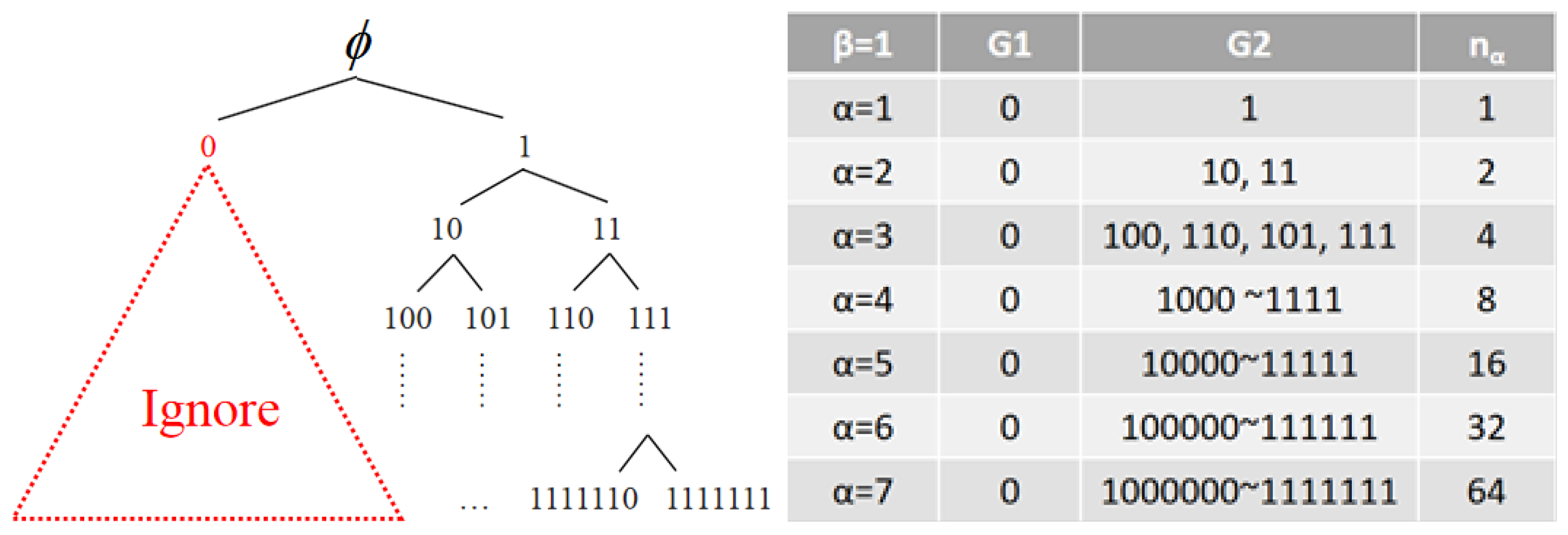
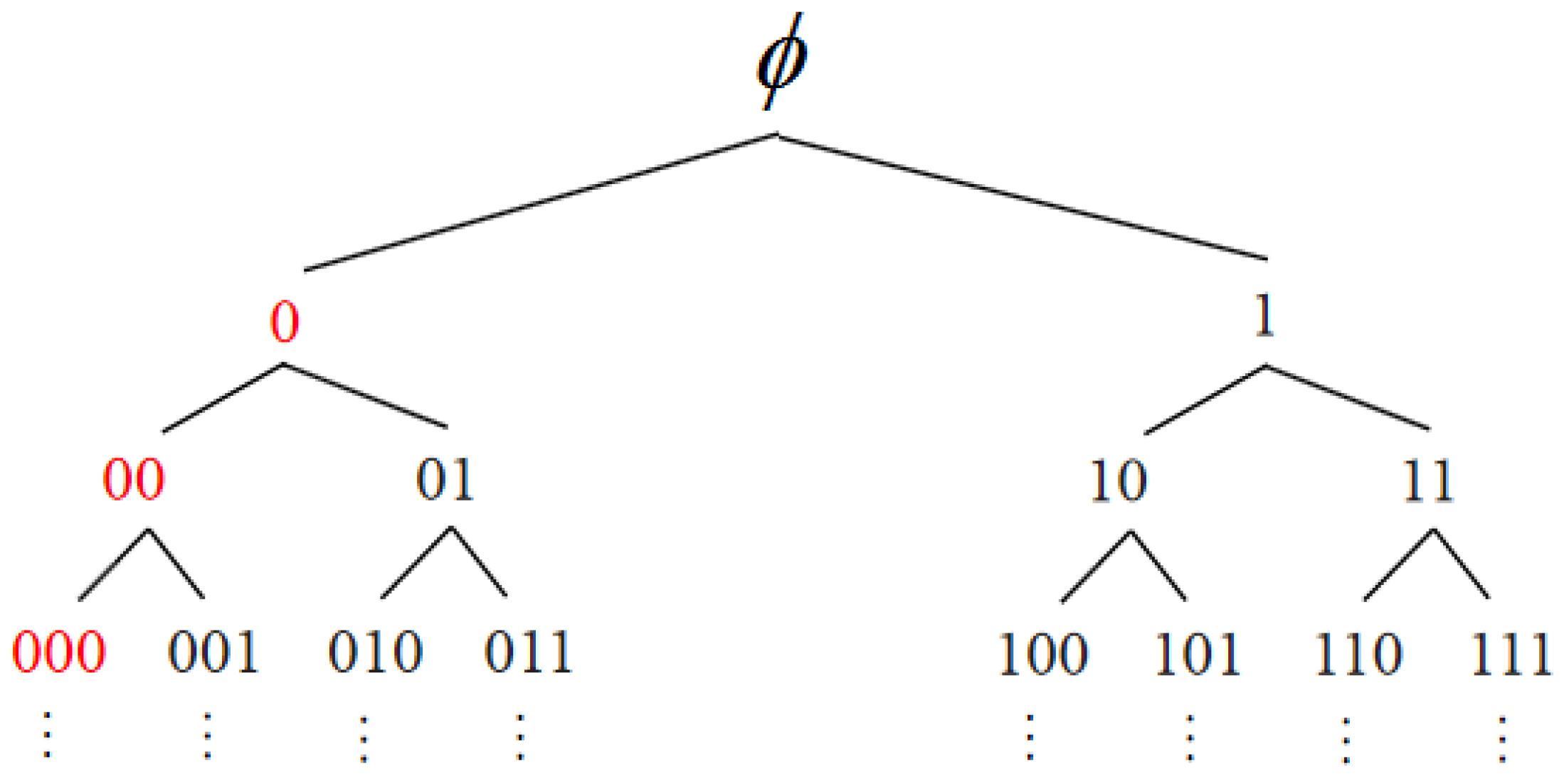
The reversible data hiding in encrypted image using PBTL, proposed by Yi and Zhou [26], first selects sampling pixels of an image as the reference pixels. The other pixels are classified into two different groups, the non-embeddable group G1 and the embeddable group G2, and labeled with PBTL. Figure 1 shows a complete binary tree. The principle of PBTL is to label G1 with the code of a leftmost node as the red codes in Figure 1 and label G2 with the other decodable/distinguishable codes. Each code for G2 is then used to label the pixels of a specified prediction error.

The parameters $\alpha$ and $\beta$ are the lengths of codes for G2 and G1 groups, respectively. An example of $\beta =1$ is shown in Figure 2. The leftmost node with a length of 1-bit is ‘0’, which is applied to label all non-embeddable pixels. The decodable nodes are thus the descended nodes of ‘1’. The value of $\alpha$ determines the number of available nodes to label the pixels in G2. When $\alpha =1$, only the code ‘1’ can be used. As the value of $\alpha$ increases, the number of available codes also increases as listed in Figure 2. For the case of $\beta =2$, the code ‘00’ is applied to label G1. The decodable codes are therefore the descended nodes of ‘01’, ‘10’, and ‘11’. When the chosen value of $\alpha$ is greater than 2, more codes are available to label G2 as listed in Figure 3. A value of is also applicable. Only the leftmost node should be reserve to make the G2 codes decodable. The number of available codes for G2 is denoted with $n_{\alpha }$ and can be analyzed to be

$$n_{\alpha }=\left\{\begin{array}{c}{2}^{\alpha }-1,\alpha \le \beta ,\\ \left(2^{\beta }-1\right)\times 2^{\alpha -\beta },\alpha >\beta .\end{array}\right.$$

(1)

2.2. IPBTL-RDHEI

The reversible data hiding using IPBTL [27] shares the same framework as the hiding scheme using PBTL [26]. The main difference is the reduction of reference pixels. IPBTL exploits the first row and the first column of an image as the reference pixels. Thus, the number of embeddable pixels is greatly increased. Therefore, the total payload is greater than the PBTL-based data-hiding scheme. The IPBTL-RDHEI scheme consists of the following two phases.

2.2.1. Pixel Labeling and Data Hiding

As mentioned, the first row and the first column of the cover image are selected as the reference pixels. Then, the prediction errors of the remaining pixels are calculated. After obtaining the prediction error array, the whole image is encrypted with the image encryption key and each non-reference pixel is labeled according to its prediction error. Finally, the secret information is encrypted with the data-hiding key and embedded into the predefined embeddable space.

2.2.2. Data Extraction and Image Recovery

In the data-extraction phase, the embeddable space can be determined according to the labels in the encrypted image. Then, the secret data are extracted and decrypted with the data-hiding key. To recover the image, the marked encrypted image is first decrypted with the image encryption key. Then, the original image can be exactly recovered according to the prediction errors indicated by the labels.

3. Proposed EPBTL-RDHEI

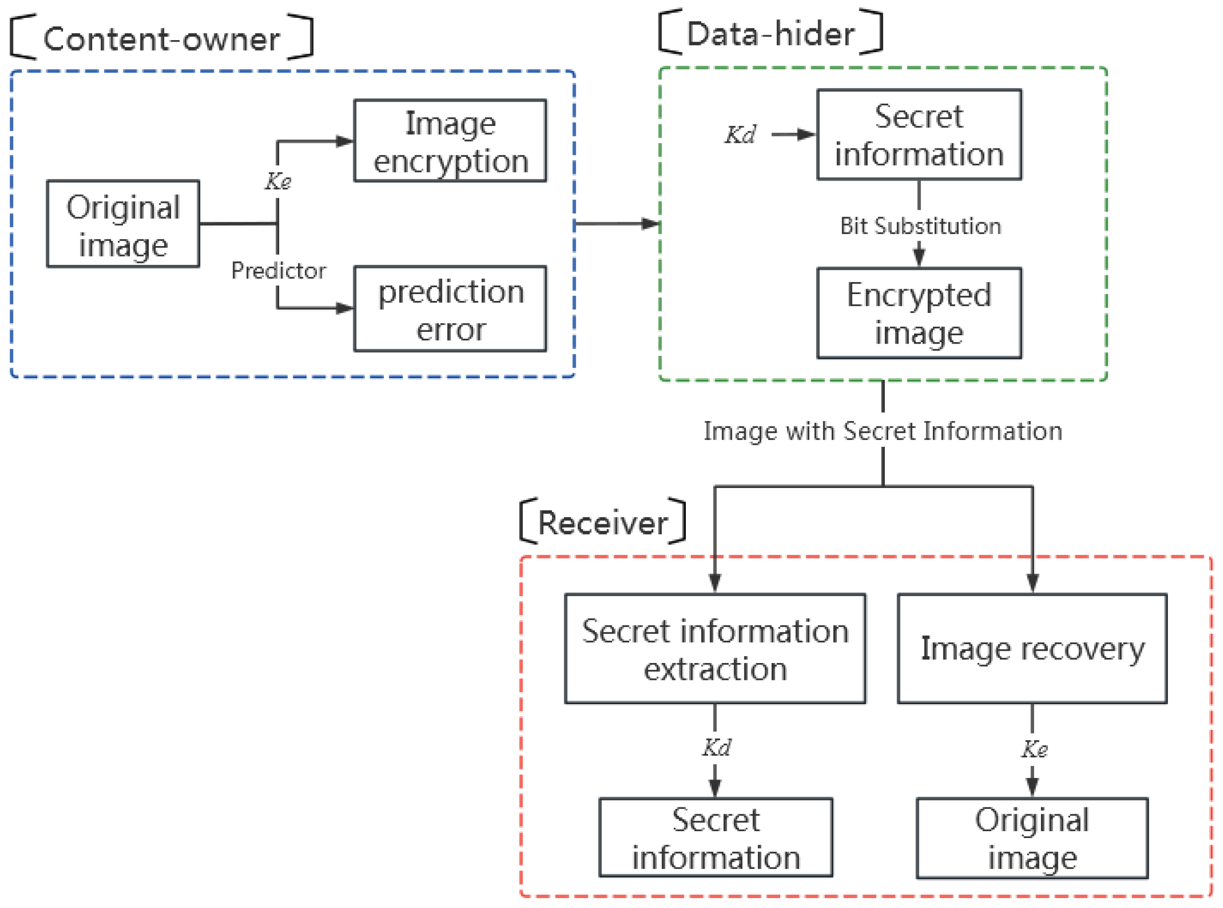
The proposed reversible data hiding in encrypted images with extended parametric binary tree labeling (EPBTL-RDHEI) consists of three phases, namely (1) the image encryption and pixel grouping, (2) the pixel labeling and data hiding, and (3) the data extraction and image recovery. As shown in Figure 4, in the first phase, the content owner uses a predictor to calculate the prediction errors of the cover image. Then, the image is encrypted with the encryption key $k_e$ and the pixels are grouped according to the prediction errors. In the second phase, the data hider embeds the secret information, which is encrypted by the data-hiding key $k_d$, into the encrypted image by bit substitution. In the third phase, the receiver can separately use the data-hiding key $k_d$ to correctly extract the secret information from the encrypted image, or use the encryption key $k_e$ to recover the original image based on the prediction errors. The receiver can do both when the two keys are in hand.

3.1. Image Encryption and Pixel Grouping

There are three steps in this phase, namely the prediction error calculation, the image encryption, and the pixel grouping. Details are as follows.

3.1.1. Prediction Error Calculation

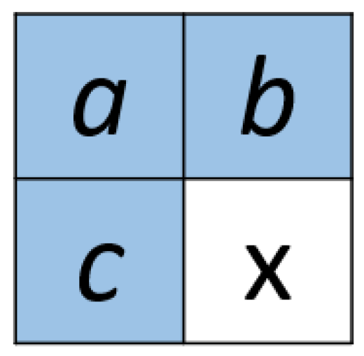
Our approach shares the same framework as IPBTL [27]. The top row and left column of the original image are selected as the reference pixels. The values of the remaining pixels are predicted based on the reference pixels. The median-edge detector (MED) [12] is applied to predict pixel values in the raster scan order. The prediction of MED is illustrated in Figure 5. The pixel marked ‘x’ is predicted using pixels ‘a’, ‘b’, and ‘c’. The predicted value $p_x$ is given by

$$p_x=\left\{\begin{array}{c}max\left(b,c\right),a\le min\left(b,c\right),\\ min\left(b,c\right),a\ge max\left(b,c\right),\\ b+c-a,otherwise.\end{array}\right.$$

(2)

The prediction error is therefore given by

$$e=x-p_x.$$

(3)

Figure 6 shows an example of image I to calculate the prediction error. The subsequent demonstrations of detailed operations in Section 3 are based on this original image I.

3.1.2. Image Encryption

The stream cypher is adopted as the image encryption scheme. A pseudo-random matrix R is generated with the encryption key $k_e$. Then, the bitwise exclusive-or (XOR) operation is applied as

$$x_e^k(i,j)=x^k(i,j)\oplus r^k(i,j),k=1,2,\dots ,8,$$

(4)

where ⊕ is the XOR operation, the notations i and j are the row and column indices of the image, and k denotes the bit index of a pixel. The resulting pixel array is the encrypted image $I_e$ as shown in Figure 7.

3.1.3. Pixel Grouping

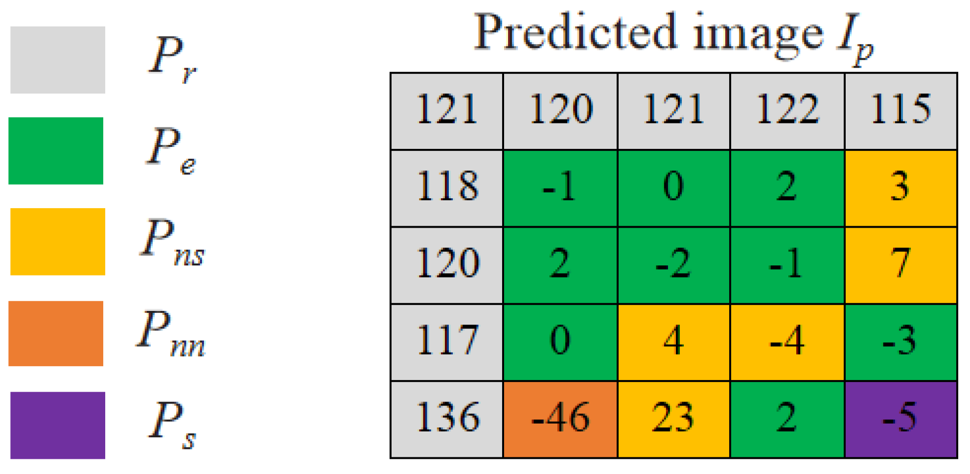
The pixels in the encrypted image $I_e$ are divided into four groups, namely the reference pixel group $P_r$, the special pixel group $P_s$, the embeddable pixel group $P_e$, and the non-embedded pixel group $P_n$. The non-embeddable pixel group $P_n$ is further divided into the self-recordable subgroup $P_{ns}$ and the non-recordable subgroup $P_{nn}$ according to their prediction errors. $P_r$ is composed of the pixels in the top row and the left column of the image. The pixel at the bottom right corner of the image is chosen as the only pixel in the group $P_s$ and is used to record parameter values $\alpha$ and $\beta$.

The remaining pixels are classified into groups $P_e$, $P_{ns}$, and $P_{nn}$ based on their prediction errors. The embeddable pixel group $P_e$ corresponds to the group G2 in PBTL. Recall that the number of different codes in G2 is defined in Equation (1). Thus, we exploit these G2 codes to label the embeddable pixels $P_e$ of prediction errors within the range defined by

$$⌈-\frac{n_a}{2}⌉\le e_i\le ⌊\frac{n_a-1}{2}⌋.$$

(5)

For a non-embeddable pixel, if its prediction error can be encoded in $\left(8-\beta \right)$ bits, it is classified as a $P_{ns}$ pixel. Otherwise, it is classified as a $P_{nn}$ pixel. The precise range of prediction error for the group $P_{ns}$ is given in Equation (6). Figure 8 gives an illustrative example of pixel grouping for $\alpha =3$ and $\beta =2$.

$$\begin{array}{c}\hfill e_i\left(P_n\right)\in \left(-2^{7-\beta }-\frac{\left(2^{\beta }-1\right)\times 2^{\alpha -\beta }}{2}+1,\left.-\frac{\left(2^{\beta }-1\right)\times 2^{\alpha -\beta }}{2}\right]\right.\cup \\ \hfill \left[\frac{\left(2^{\beta }-1\right)\times 2^{\alpha -\beta }}{2}-1,\left.\frac{\left(2^{\beta }-1\right)\times 2^{\alpha -\beta }}{2}+2^{7-\beta }-2\right).\right.\end{array}$$

(6)

3.2. Pixel Labeling and Data Hiding

After classifying the pixels into groups, the encrypted image is ready for labeling. This subsection presents the details for pixel labeling and data hiding.

3.2.1. Recording Parameters

The parameter values of $\alpha$ and $\beta$ are converted into 4-bit and 3-bit, respectively. Then, the 7 bits is recorded to the special pixel $P_s$. The remaining 1 bit is reserved to record the version code, which will be explained later. The replaced eight bits of encrypted pixel value are treated as auxiliary information and appended to the front of secret data.

3.2.2. Labeling of Embeddable Group

The labeling of embeddable pixels follows PBTL. The mapping of prediction errors to the label codes for $\alpha =3$ and $\beta =2$ is given in

Table 1. Coding table of the prediction error when $\alpha =3$ and $\beta =2$.

${\mathit{P}}_{\mathit{n}}$	${\mathit{P}}_{\mathit{e}}$
00	2	1	0	−1	−2	−3
	111	110	101	100	011	010

. An example of pixel labeling is illustrated in Figure 9.

According to Table 1, the pixels with prediction error ranged from −3 to 2 are embeddable. The lowest three bits of an embeddable pixel are used to record the label code. All label codes are recorded backward. For example, the prediction error −1 maps to ‘100’. Thus, ‘001’ is recorded to the lowest three bits of the pixel.

The mapping table in Table 1 is not a fixed version. In general, the histogram of prediction error decreases with increasing absolute error. For $\alpha =3$ and $\beta =2$, there are six G2 codes. Therefore, two possible ranges of prediction error can be selected, i.e., −3 to 2 or −2 to 3. We can select a better version according to the error distribution of the given image.

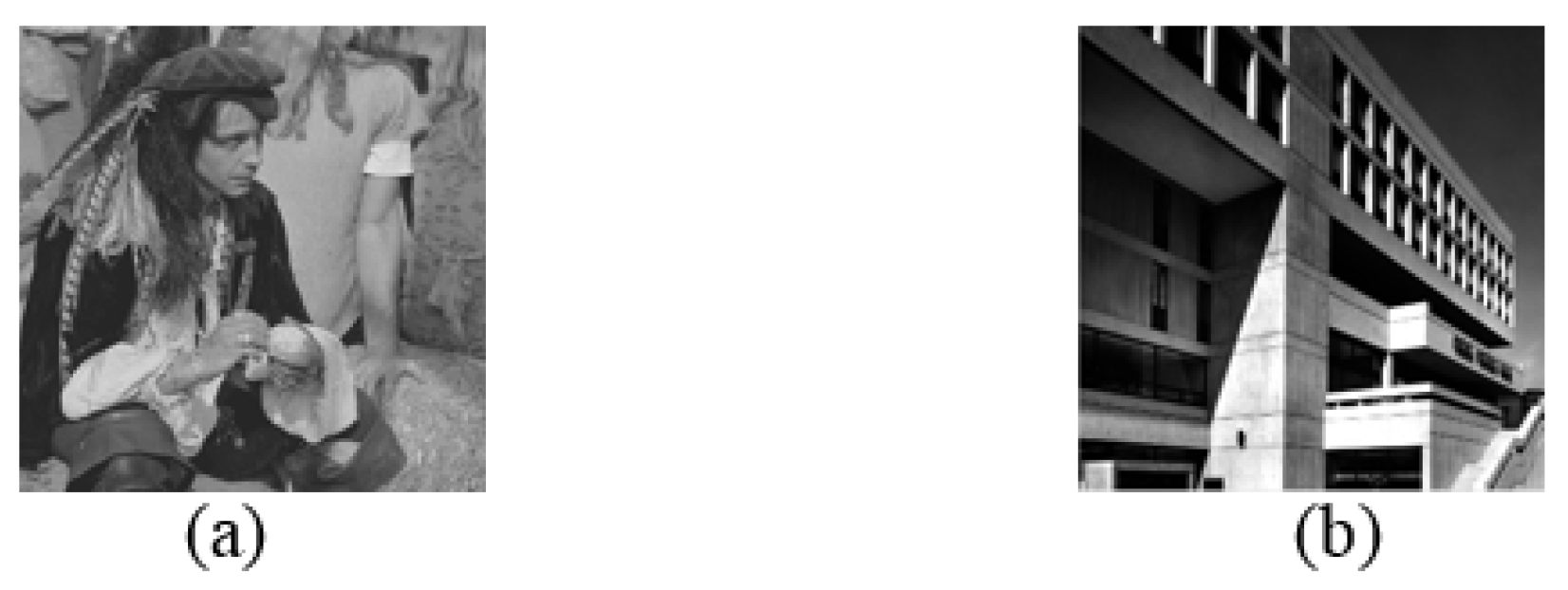
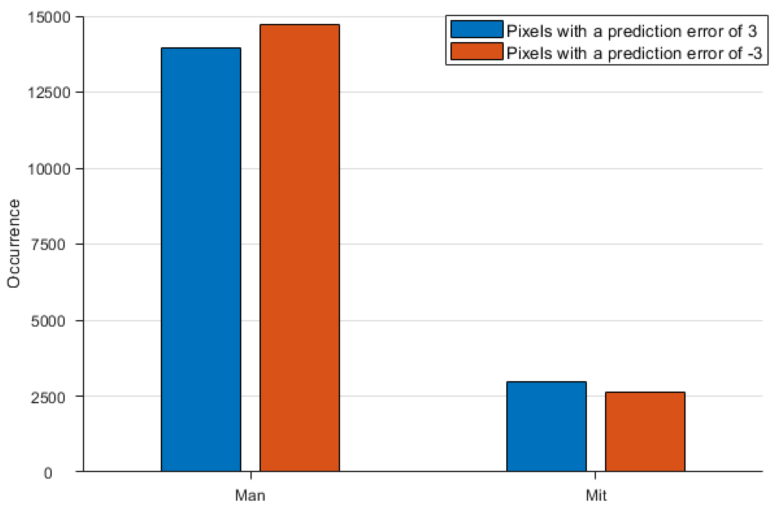
Figure 10 shows two test images and Figure 11 is the histogram of prediction error at −3 and 3 for the two images. As shown in the plot, the number of pixels with a prediction error of −3 is greater than the number of pixels with an error of 3. But the other image behaves quite contrary. Thus, we select the version of −3 to 2 for image ‘Man’ and the version of −2 to 3 for image ‘Mit’. The bit of version code is used to indicate the actual version applied. For the example given in Figure 9, we record the parameters and version code with ‘0011’ for, ‘010’ for, and ‘0’ for the version of −3 to 2.

3.2.3. Labeling of Non-Embeddable Group

Our labeling of the non-embeddable pixels is completely different from PBTL or IPBTL. By extending the representation range of prediction error, we further divide the non-embeddable group into the self-recordable group $P_{ns}$ and the non-recordable group $P_{nn}$. When the prediction error satisfies Equation (6), it can be represented with $\left(8-\beta \right)$ bits and recorded in its current position and classified as a self-recordable pixel.

Suppose $\alpha =3$, $\beta =2$, and the embeddable range of prediction error is $-e_{min}$ to $+e_{max}$. Then, the $8-\beta =6$ bits are used to represent prediction error of a self-recordable pixel. The leading bit is used as sign bit and the remaining five bits are used to represent $e-e_{min}$ for $e<0$ or $e-e_{max}$ for $e>0$. For example, a non-embeddable pixel with $e=3$ is represented as ‘10000100’, where the leading code is ‘1’ for positive, ‘00001’ represents the absolute error $e-e_{max}$ and ‘00’ is the group label. Thus, no auxiliary information is required to record a self-recordable pixel.

For a non-recordable pixel in the $P_{nn}$ group, in addition to the group label ‘00’, the remaining six bits are marked with a stream of zeros ‘000000’ and the whole eight bits are recorded as a part of the auxiliary information.

3.2.4. Data Hiding

The secret data is encrypted with the data-hiding key $k_d$. After appending the auxiliary information (AI), the whole data stream is embedded into the vacated space of the embeddable pixels. The data embedding process is illustrated in Figure 12. Thus, the marked encrypted image $I_s$ is obtained.

3.3. Data Extraction and Image Recovery

To extract secret data, we first classify the pixels into groups according to the labels. Then, extract embedded data from the embeddable group. Count the number of non-recordable pixels and the special pixel and remove their corresponding auxiliary information from the head of the data stream. Finally, decrypt the secret data with the data-hiding key.

To recover image, the parameters and the version code are decoded from the special pixel first. Then, pixels are classified into groups according to the labels. Extract the embedded data from the embeddable group and retrieve the auxiliary information to recover the special pixel and the non-recordable pixels. The reference pixels are recovered with the image encryption key. Finally, the embeddable pixels and the self-recordable pixels are recovered according to the recorded prediction errors. Thus, the original image can be completely restored.

4. Experimental Results

To evaluate the performance of the proposed scheme, we conducted experiments on security analysis, image quality, embedding capacity and comparison of state-of-the-art schemes. As shown in Figure 13, we chose four standard grayscale images as the test images in the experiment. More, the datasets UCID [28], BOSSbase [29], and BOWS-2 [30] were used in the experiments to verify whether the scheme can be applied to most images.

4.1. Security Analysis

Security analysis is a very important step to test the ability of a scheme to resist attacks. Then, we will test the security of the scheme in two parts: the histogram of image and the information entropy.

4.1.1. Histogram of Images

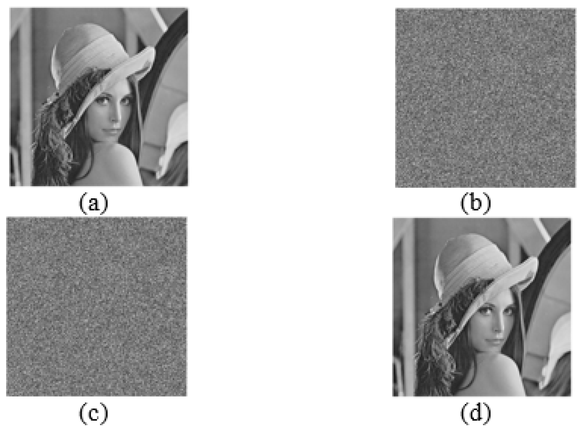
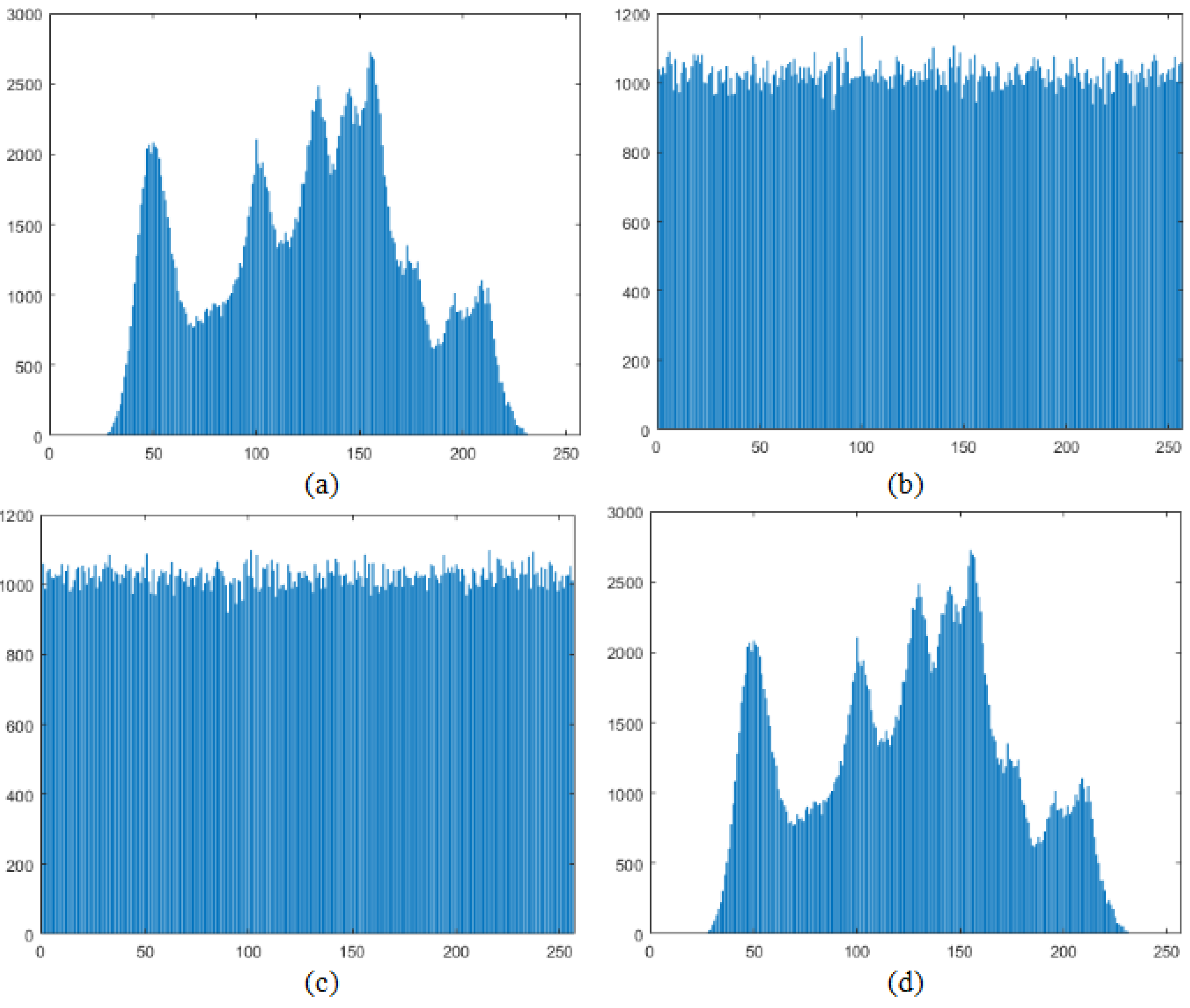
In order to test the pixel distribution of the images generated in different phases, we give the corresponding experimental results and histograms for Lena as an example, as shown in Figure 14 and Figure 15.

As can be seen in Figure 15, the original image (a) and the recovered image (d) in Figure 14 are the same, indicating that the proposed scheme can recover the original image losslessly. In addition, the pixel distribution of the encrypted image (b) and the embebded encrypted image (c) is even and chaotic that is different from the pixel distribution of the original image. It can be concluded that it is almost impossible to obtain the information of the original image from the encrypted image.

4.1.2. Entropy of Image

The advantage of encrypted images is that the information patterns about the pixels cannot be inferred. Therefore, to further verify the security of the proposed scheme, we use information entropy to calculate the pixel randomness of the images at different phases. The information entropy can be obtained from Equation (7), where s represents the gray level of an image pixel, $p\left(s_i\right)$ represents the relative probability of a particular gray level $s_i$ in the image, and $2^n$ represents the total number of gray levels.

$$\begin{array}{c}\hfill H\left(s\right)=-\sum _{i=0}^{2^n-1}p\left(s_i\right)·{log}_2\left(p\left(s_i\right)\right).\end{array}$$

(7)

We conducted experiments using the test images in Figure 13 including Lena, Man, Jetplane and Baboon.

Table 2. Information entropy of the image at different stages.

Image	Original Image	Encrypted Image	Embedded Encrypted Image
Lena	7.4455	7.9985	7.9865
Man	7.1926	7.9862	7.9952
Jetplane	6.6776	7.9923	7.9912
Baboon	7.3899	7.9965	7.9936

shows the information entropy of the test images at different stages, from which we can see that both the encrypted image and the embedded encrypted image are very close to 8. The theoretical maximum of the information entropy is 8, and the closer to 8 the higher the randomness of the image is. This shows that the proposed scheme security is reliable.

4.2. Image Quality Assessment

It is important to assess the quality of the recovered image compared to the original image and the encrypted image. If the recovered image is different from the original cover image, full reversibility is not ensured. If the quality of the encrypted image is high, the scheme is poorly encrypted and there is a risk of information leakage.

The PSNR and the SSIM are often used to evaluate the quality of an image after it has been processed compared to the original image. the PSNR is the peak signal to noise ratio, which is the ratio between the maximum possible power of the signal and the power of the corrupted noise that affects the fidelity of its representation. The unit is decibels (dB). The higher the PSNR, the closer the image is to the original. The SSIM is the Structural Similarity Index. It is a measure of the quality of images based on visual perception and takes a value from 0 to 1. The SSIM value is 1 when the two images are structurally identical.

Four test images in Figure 13 were used for the experiment.

Table 3. PSNR and SSIM between the original image and recovered image.

Image	Lena	Man	Jetplane	Baboon
PSNR (dB)	∞	∞	∞	∞
SSIM	1	1	1	1

shows the PSNR and SSIM for the original and recovered images, where PSNR is ∞ and SSIM is 1. This indicates that the proposed scheme can be made fully reversible.

Table 4. PSNR and SSIM between the original image and embedded encrypted image.

Image	Lena	Man	Jetplane	Baboon
PSNR (dB)	9.1231	7.5832	8.0899	5.9632
SSIM	0.0312	0.0661	0.0349	0.0310

shows a comparison of the original image and embedded encrypted image, where the PSNR does not exceed 10 and the SSIM is close to 0. This shows that the two images are so different that the proposed scheme cannot derive the original image from the embedded encrypted image.

4.3. Embedding Capacity

In order to calculate the embedding capacity of the proposed scheme, we conducted some experiments with test images and datasets. Also, state-of-the-art schemes were compared.

The embedding capacity is the total number of bits in the embedded image. Therefore the embedding rate is used to measure the embedding ability of the original image. The embedding rate represents the number of bits of information that can be embedded into each pixel, and it is measured in bits per pixel (bpp). A larger embedding rate means that the solution is more capable of embedding.

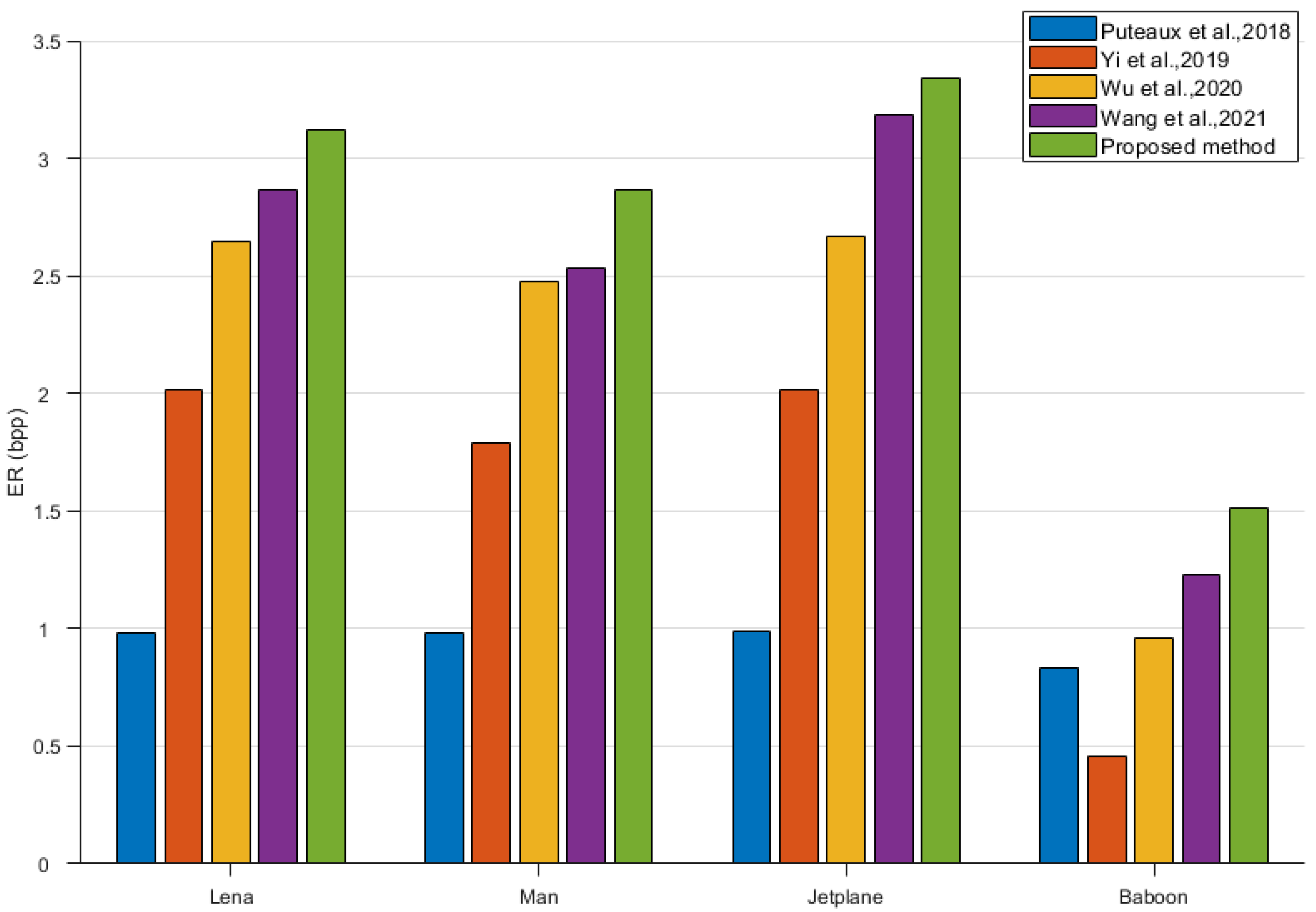
In order to obtain the highest embedding rates in the experiments, all scenarios used the best effect parameter settings. Figure 16 compares the proposed EPBTL scheme and four SOTA schemes including Puteaux et al. [23], Wang et al. [25], Yi et al. [26], Wu et al. [27] on the four testing images including Lena, Man, Jetplane and Baboon in terms of embedding rate. As can be seen in the four test images, the proposed scheme shows varying degrees of improvement in embedding rate over the other four SOTA schemes. The images ’Jetplane’ and ’Lena’ both have an embedding rate of over 3.0 bpp, which is a significant change. The image ’Jetplane’ has a smaller increase compared to the other three images. This is because the prediction errors for the pixels of the image ’Jetplane’ fall less in the self-recordable subgroup ($P_{ns}$). It leads to an increase in the data that needs to be recorded by the auxiliary information.

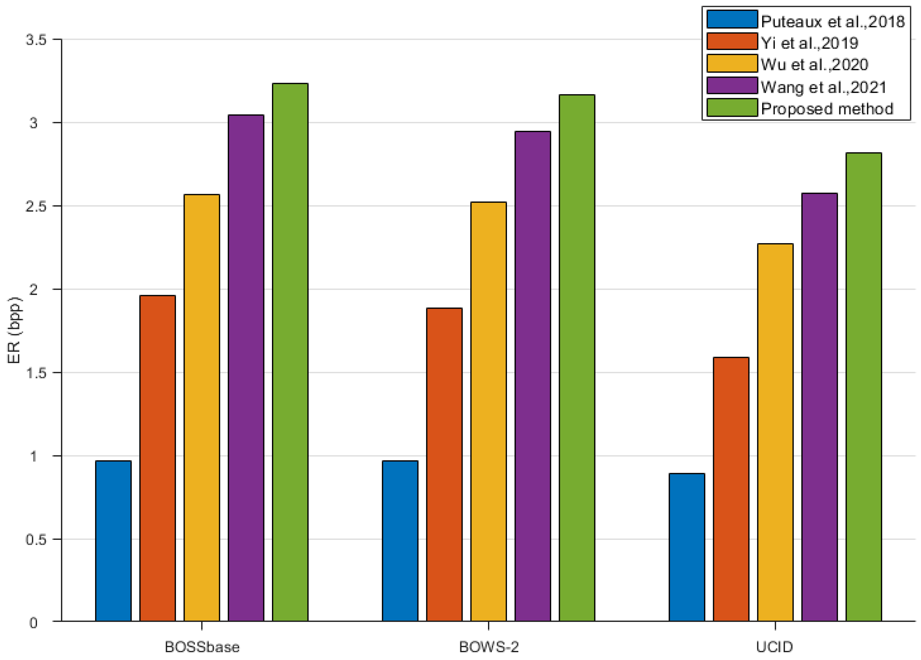
To verify the generality of the scheme, we compare this schemes on the three datasets including UCID [28], BOSSbase [29], and BOWS-2 [30] in terms of average embedding rate. As can be seen in Figure 17, in the datasets BOSSbase and BOWS-2, the proposed scheme also has an embedding rate of more than 3.0 bpp. The embedding rate also improved on the dataset UCID. This indicates that the proposed scheme has a higher embedding rate than the other schemes in the experiment with random images.

Table 5. The embedding rate of the IPBTL-RDHEI scheme when $\beta =2$ and $\alpha =2\sim 7$.

$\left(\mathit{\alpha },\mathit{\beta }\right)$	$\left(1,2\right)$	$\left(2,2\right)$	$\left(3,2\right)$	$\left(4,2\right)$	$\left(5,2\right)$	$\left(6,2\right)$	$\left(7,2\right)$
Lena	/	0.3912	1.6654	2.6812	2.6413	1.9245	0.9945
Man	/	/	0.8173	2.0054	2.4745	1.9015	0.9831
Jetplane	/	1.5354	2.6098	3.0233	2.6745	1.9245	0.9945
Baboon	/	/	/	0.2015	0.9613	1.2445	0.8615

,

Table 6. The embedding rate of the HPBTL scheme when $\beta =2$ and $\alpha =2\sim 7$.

$\left(\mathit{\alpha },\mathit{\beta }\right)$	$\left(1,2\right)$	$\left(2,2\right)$	$\left(3,2\right)$	$\left(4,2\right)$	$\left(5,2\right)$	$\left(6,2\right)$	$\left(7,2\right)$
Lena	/	1.1949	2.5717	3.0926	2.7605	1.9392	0.9736
Man	/	1.2231	2.4553	2.8687	2.6002	1.8743	0.9398
Jetplane	/	1.8044	3.2733	3.3413	2.7848	1.9380	0.9735
Baboon	/	0.1008	0.7210	1.2117	1.5125	1.3134	0.6282

,

Table 7. The embedding rate of the IPBTL-RDHEI scheme when $\beta =3$ and $\alpha =2\sim 7$.

$\left(\mathit{\alpha },\mathit{\beta }\right)$	$\left(1,3\right)$	$\left(2,3\right)$	$\left(3,3\right)$	$\left(4,3\right)$	$\left(5,3\right)$	$\left(6,3\right)$	$\left(7,3\right)$
Lena	/	/	1.7045	2.7872	2.6754	1.9445	0.9974
Man	/	/	0.6545	2.0964	2.5517	1.9945	0.9854
Jetplane	/	0.9855	2.6945	3.0589	2.6945	1.9367	0.9845
Baboon	/	/	/	/	0.8745	1.2502	0.8854

and

Table 8. The embedding rate of the HPBTL scheme when $\beta =3$ and $\alpha =2\sim 7$.

$\left(\mathit{\alpha },\mathit{\beta }\right)$	$\left(1,3\right)$	$\left(2,3\right)$	$\left(3,3\right)$	$\left(4,3\right)$	$\left(5,3\right)$	$\left(6,3\right)$	$\left(7,3\right)$
Lena	/	/	2.4214	3.1249	2.6615	1.8012	0.8248
Man	/	/	2.2063	2.7858	2.4203	1.6445	0.6934
Jetplane	/	/	3.1450	3.3132	2.6863	1.8116	0.8370
Baboon	/	/	/	0.5392	0.7967	0.5228	/

show the embedding rate of the IPBTL-RDHEI scheme and in the proposed EPBTL scheme when $\alpha =2\sim 7$, and $\beta =2$ and 3. We only need to pay attention to the optimal value of each image in all situations. The reason for choosing $\beta =2$, 3, $\alpha =2\sim 7$ is that the experiments can achieve the better embedding rate at this configuration.

In Table 5, Table 6, Table 7 and Table 8, “/” indicates that it is not possible to embed information in this case. The bold data are the best embedding rate for the images. The embedding rates of these four images in the proposed EPBTL scheme can reach 3.1249, 2.8687, 3.3413, and 1.5125, respectively, which have an increase of about 0.3 bpp compared with the results of the IPBTL-RDHEI scheme, i.e., 2.7872, 2.5517, 3.0589, and 1.2502, respectively.

The increase of data payload is due to the reduction of the size of auxiliary information. The reduction in auxiliary information is due to the fact that the remaining $8-\beta$ bits of the pixel point in the $P_{ns}$ group are used to record the prediction error for that pixel point. The prediction error can recover the value of that pixel so that the auxiliary information does not need to record the original pixel value of that pixel. Because of the high number of pixels belonging to the $P_{ns}$ group, there is a significant embedding rate improvement in the proposed EPBTL scheme.

5. Conclusions

We propose a reversible data-hiding scheme in encrypted images with the extended parametric binary tree labeling. By extending the representation range of prediction error, most of the non-embeddable pixels turn to be self-recordable. Thus, the required auxiliary information is greatly reduced and the data payload is significantly improved. Experimental results show that the proposed EPBTL scheme outperforms state-of-the-art schemes in embedding rate. Experimental values under different parameter settings are investigated. The data extraction and image recovery can be executed separately, which is beneficial for the applications based on the cloud storage. Security level of the proposed scheme is also analyzed. Our future work will focus on the improvement of robustness to different security attacks.

References

1. Bailey, K.; Curran, K. An evaluation of image based steganography methods. Multimed. Tools Appl. 2006, 30, 55–88. [Google Scholar] [CrossRef]
2. Megías, D.; Mazurczyk, W.; Kuribayashi, M. Data Hiding and Its Applications: Digital Watermarking and Steganography. Appl. Sci. 2021, 11, 10928. [Google Scholar] [CrossRef]
3. Kim, C.; Shin, D.; Yang, C.; Leng, L. Data Hiding Method for Color AMBTC Compressed Images Using Color Difference. Appl. Sci. 2021, 11, 3418. [Google Scholar] [CrossRef]
4. Ni, Z.; Shi, Y.-Q.; Ansari, N.; Su, W. Reversible data hiding. IEEE Trans. Circuits Syst. Video Technol. 2006, 16, 354–362. [Google Scholar] [CrossRef]
5. Luo, L.; Chen, Z.; Chen, M.; Zeng, X.; Xiong, Z. Reversible Image Watermarking Using Interpolation Technique. IEEE Trans. Inf. Forensics Secur. 2009, 5, 187–193. [Google Scholar] [CrossRef]
6. Li, X.; Zhang, W.; Gui, X.; Yang, B. A Novel Reversible Data Hiding Scheme Based on Two-Dimensional Difference-Histogram Modification. IEEE Trans. Inf. Forensics Secur. 2013, 8, 1091–1100. [Google Scholar] [CrossRef]
7. Tian, J. Reversible data embedding using a difference expansion. IEEE Trans. Circuits Syst. Video Technol. 2003, 13, 890–896. [Google Scholar] [CrossRef]
8. Alattar, A. Reversible Watermark Using the Difference Expansion of a Generalized Integer Transform. IEEE Trans. Image Process. 2004, 13, 1147–1156. [Google Scholar] [CrossRef] [PubMed]
9. Thodi, D.M.; Rodriguez, J.J. Expansion Embedding Techniques for Reversible Watermarking. IEEE Trans. Image Process. 2007, 16, 721–730. [Google Scholar] [CrossRef] [PubMed]
10. Kim, C.; Yang, C.-N.; Baek, J.; Leng, L. Survey on Data Hiding Based on Block Truncation Coding. Appl. Sci. 2021, 11, 9209. [Google Scholar] [CrossRef]
11. Jaya Prakash, S.; Mahalakshmi, K. Improved reversible data hiding scheme employing dual image-based least significant bit matching for secure image communication using style transfer. Vis. Comput. 2021, 38, 4129–4150. [Google Scholar] [CrossRef]
12. Fridrich, J.; Goljan, M.; Du, R. Lossless Data Embedding—New Paradigm in Digital Watermarking. EURASIP J. Adv. Signal Process. 2002, 2002, 986842. [Google Scholar] [CrossRef]
13. Hung, C.-C.; Lin, C.-C.; Wu, H.-C.; Lin, C.-W. A Study on Reversible Data Hiding Technique Based on Three-Dimensional Prediction-Error Histogram Modification and a Multilayer Perceptron. Appl. Sci. 2022, 12, 2502. [Google Scholar] [CrossRef]
14. Li, X.; Li, J.; Li, B.; Yang, B. High-fidelity reversible data hiding scheme based on pixel-value-ordering and prediction-error expansion. Signal Process 2012, 93, 198–205. [Google Scholar] [CrossRef]
15. Kim, C.; Shin, D.; Leng, L.; Yang, C.-N. Lossless data hiding for absolute moment block truncation coding using histogram modification. J. Real-Time Image Process. 2016, 14, 101–114. [Google Scholar] [CrossRef]
16. Puech, W.; Chaumont, M.; Strauss, O. A reversible data hiding method for encrypted images. In Proceedings of the Security, Forensics, Steganography, and Watermarking of Multimedia Contents X, Bellingham, WA, USA, 18 March 2008; Volume 6819, p. 68191E. [Google Scholar] [CrossRef]
17. Zhou, J.; Sun, W.; Dong, L.; Liu, X.; Au, O.C.; Tang, Y.Y. Secure Reversible Image Data Hiding Over Encrypted Domain via Key Modulation. IEEE Trans. Circuits Syst. Video Technol. 2015, 26, 441–452. [Google Scholar] [CrossRef]
18. Qian, Z.; Zhang, X.; Wang, S. Reversible data hiding in encrypted JPEG bitstream. IEEE Trans. Multimed. 2014, 16, 1486–1491. [Google Scholar] [CrossRef]
19. Qin, C.; Qian, X.; Hong, W.; Zhang, X. An efficient coding scheme for reversible data hiding in encrypted image with redundancy transfer. Inf. Sci. 2019, 487, 176–192. [Google Scholar] [CrossRef]
20. Liao, X.; Li, K.; Yin, J. Separable data hiding in encrypted image based on compressive sensing and discrete fourier transform. Multimed. Tools Appl. 2016, 76, 20739–20753. [Google Scholar] [CrossRef]
21. Zhang, X. Separable Reversible Data Hiding in Encrypted Image. IEEE Trans. Inf. Forensics Secur. 2011, 7, 826–832. [Google Scholar] [CrossRef]
22. Ma, K.; Zhang, W.; Zhao, X.; Yu, N.; Li, F. Reversible Data Hiding in Encrypted Images by Reserving Room Before Encryption. IEEE Trans. Inf. Forensics Secur. 2013, 8, 553–562. [Google Scholar] [CrossRef]
23. Puteaux, P.; Puech, W. An Efficient MSB Prediction-Based Method for High-Capacity Reversible Data Hiding in Encrypted Images. IEEE Trans. Inf. Forensics Secur. 2018, 13, 1670–1681. [Google Scholar] [CrossRef]
24. Puyang, Y.; Yin, Z.; Qian, Z. Reversible data hiding in encrypted images with two-MSB prediction. In Proceedings of the 2018 IEEE International Workshop on Information Forensics and Security (WIFS), Hong Kong, China, 11–13 December 2018; pp. 1–7. [Google Scholar]
25. Wang, R.; Wu, G.; Wang, Q.; Yuan, L.; Zhang, Z.; Miao, G. Reversible Data Hiding in Encrypted Images Using Median Edge Detector and Two’s Complement. Symmetry 2021, 13, 921. [Google Scholar] [CrossRef]
26. Yi, S.; Zhou, Y. Separable and Reversible Data Hiding in Encrypted Images Using Parametric Binary Tree Labeling. IEEE Trans. Multimed. 2019, 21, 51–64. [Google Scholar] [CrossRef]
27. Wu, Y.; Xiang, Y.; Guo, Y.; Tang, J.; Yin, Z. An Improved Reversible Data Hiding in Encrypted Images Using Parametric Binary Tree Labeling. IEEE Trans. Multimed. 2019, 22, 1929–1938. [Google Scholar] [CrossRef]
28. Schaefer, G.; Stich, M. UCID: An uncompressed color image database. In Storage and Retrieval Methods and Applications for Multimedia 2004; SPIE: San Jose, CA, USA, 2003; Volume 5307, pp. 472–480. [Google Scholar] [CrossRef]
29. Bas, P.; Filler, T.; Pevný, T. “Break our steganographic system”: The ins and outs of organizing BOSS. In International Workshop on Information Hiding; Springer: Berlin/Heidelberg, Germany, 2011; pp. 59–70. [Google Scholar] [CrossRef] [Green Version]
30. Bas, P.; Furon, T. Image Database of BOWS-2. Available online: http://bows2.ec-lille.fr/ (accessed on 17 July 2007).
Figure 1. Binary code distribution based on a complete binary tree.
Applsci 13 02458 g001
Figure 2. An example of flag bit selection when β = 1 and α = 1 to 7.
Applsci 13 02458 g002
Figure 3. An example of flag bit selection when β = 2 and α = 1 to 7.
Applsci 13 02458 g003
Figure 4. Procedure of the proposed method.
Applsci 13 02458 g004
Figure 5. Median-edge detector.
Applsci 13 02458 g005
Figure 6. Example of the prediction error.
Applsci 13 02458 g006
Figure 7. Image encryption.
Applsci 13 02458 g007
Figure 8. Pixel grouping.
Applsci 13 02458 g008
Figure 9. The labeled encrypted image generation process.
Applsci 13 02458 g009
Figure 10. Testing images: (a) Man, (b) Mit.
Applsci 13 02458 g010
Figure 11. The numbers of the pixels with two different prediction errors.
Applsci 13 02458 g011
Figure 12. AI and secret data hiding.
Applsci 13 02458 g012
Figure 13. The test images: (a) Lena, (b) Man, (c) Jetplane, (d) Baboon.
Applsci 13 02458 g013
Figure 14. The different phases of EPBTL on Lena image: (a) Original image, (b) Encrypted image, (c) Embebded encrypted image, (d) Recovered image.
Applsci 13 02458 g014
Figure 15. The histograms of images at different phases of EPBTL on Lena: (a) Histogram of the original image, (b) Histogram of the encrypted image, (c) Histogram of the embebded encrypted image, (d) Histogram of the recovered image.
Applsci 13 02458 g015
Figure 16. The comparison of the embedding rates of the different schemes on the test images includes Puteaux et al. [23], Wang et al. [25], Yi et al. [26], Wu et al. [27] and Proposed method.
Applsci 13 02458 g016
Figure 17. The comparison of the average embedding rates of the different schemes on the datasets includes Puteaux et al. [23], Wang et al. [25], Yi et al. [26], Wu et al. [27] and Proposed method.
Applsci 13 02458 g017