Effect of Finite Element Method (FEM) Mesh Size on the Estimation of Concrete Stress–Strain Parameters

Abstract

In this research, two components were developed jointly: On the one hand, an experimental plan was created to obtain specific variables of the concrete and serve as a reference for the second model, a numerical and computational type created to address the variability in parameters, such as the elasticity and flow of coarse aggregate and mortar. The experimental work reproduced a specific gradation with a 1” nominal maximum size TMN on spheroidal-shaped particles. To address the diversity of limestone in the national territory, rocks were extracted from five calcareous areas of the country, which were transformed through different activities from lamination and turning with different bits to being carved into spheres until the reference gradation formed. The next stage consisted of determining the mechanical and stress–strain properties of both the mortar and coarse aggregate. In the case of mortar, the compressive stress was obtained from 50 mm × 50 mm × 50 mm cubes and the modulus of elasticity from 100 mm × 200 mm cylinders; for the coarse aggregate, the compressive stress was obtained through tests on cylinders of the calcareous rock used to form the spherical aggregate particles. The materials were mixed according to a previous proportioning for f′_c = 28 MPa and cast in cylinders of 100 mm × 200 mm. Finally, the compressive stress and the modulus of elasticity in these specimens were determined. Separately, a computational model was created to reproduce the experimental model with the same type of materials and load conditions and thereby estimate the compressive stress and modulus of elasticity of the tested material. This model was developed based on finite elements simulating concrete under a two-phase model, in which the coarse aggregate phase was arranged with spheroidal particles that were assembled with the mortar paste, thus finally reproducing a concrete cylinder of 100 mm × 200 mm. Material properties, taken from experimental work, were assigned to these materials. Initially, work was carried out in the elastic range, obtaining, as a result, the modulus of elasticity E_c, and then the specimen was brought to failure, obtaining, as a result, the maximum compressive stress f′_c. To attend to the influence of the effect of the mesh size for modeling on the numerical results of both parameters, several simulations were carried out in which mesh sizes of 4.0, 3.5, 3.0, and 2.5 mm were established for the mortar and the coarse aggregate, respectively, for carrying out the modeling. The results in the computational model showed that the compressive stress turned out to be more sensitive than the modulus of elasticity to the variation in the size of the mesh. For the first, the differences between the 4 mm mesh and the 2.5 mm mesh reached 3%, but for the second, the difference only reached 1% between the results for the same meshes. When the results between the experimental and computational models were compared, we found that the experimental values had the best closeness with results in the 2.5 mm mesh.

1. Introduction

The stress–strain parameters in concrete allow us to determine both the modulus of elasticity and the compressive strength. The modulus of elasticity test is generally carried out through the American Society for Testing and Materials (ASTM C469) and in Colombia from the Colombian technical standard (NTC 4205); the compression resistance evaluation is carried out by the ASTM C49 and NTC 673 standards, respectively. The modulus of elasticity E_c of concrete, together with compressive strength, are the most commonly used concrete properties for the design of buildings and civil structures. Over time, it was decided to express stress–strain parameters as a function of these two elements. The ability to withstand loads is made possible by the concrete resistance f′_c, and the compatibility of displacements and deformations is achieved by incorporating the E_c modulus, which is responsible for rigidity.

On both parameters, there are a large number of variables that significantly affect their values, and they are both related to the concrete components and extended to the testing mechanisms. Some of them have a greater or lesser influence on the compressive stress, other factors have considerable experimental development, some have only been explained by numerical analysis, and finally, some have not yet been addressed by scientific literature.

The modulus of elasticity E_c and the compressive strength f′_c, are influenced by coarse aggregate, mortar paste, the interfacial transition zone (ITZ), and test parameters [1,2]. It is logical to expect that since the coarse aggregate represents, on average, up to 50% of the volume of the concrete, it has an important influence on the mechanical and elastic characteristics of the concrete [3].

The modulus of elasticity of concrete is strongly influenced by the modulus of elasticity of the coarse aggregate [4,5,6,7,8]. However, the maximum size of the aggregate has a much more marked degree of affectation in both parameters [9,10,11,12,13,14].

The effects of the test parameters can be summarized in the influence of the geometry of the specimen that is primarily tested on the compression stress [15,16,17,18]. The affectation of the types of ends used for the test, both in the modulus of elasticity and in compression stress, can have a small to appreciable connotation [19,20], effects that can also be noted differently with the types of mechanisms with which they are applied to perform the test [18,21,22].

All these documented affectations are addressed and valued when formulating the computational model as variables that depend on the material and the test method to which the complications of the model are added, which, in this case, is developed in the Abaqus software of finite elements. However, there are characteristics required in the formulation of the model for its operation that have an inference on the level of accuracy of the results. Complex models are expected to require a more precise definition of the mesh size and element geometry, which, in turn, is reflected in the computational cost [23] of the model used. The search for an optimal solution that concerns the size of the mesh has been required in several investigations of the use of concrete in current engineering [24,25]. However, it is possible that the optimal value sought is not available, due to the restriction in the computational economy [26], and in that sense, it is not possible, for reasons of computational costs, to achieve a mesh level in which the error obtained can be considered irrelevant. However, it is possible to establish a relationship between the different results and their minimum mesh size [27].

Different mesh sizes have been used in finite element modeling for concrete slabs subjected to impact, explosion, and fire [28,29], as well as in the analysis of solid and hollow columns under the effects of eccentric loads and compression [30]. From this relationship, we can calculate the value to which the problem will converge to with a continuous mesh. In the case of the present investigation, the reproduction of various experimental trials, along with the computational exercise, offers us the possibility of choosing the closest model responses.

In the study of concrete and its components, we need to understand that the interactions between components are hardly even null in their experimental reproduction, such as some cases from the study of the influence of the characteristics and properties of the interface on the resistance parameters of the concrete. For this reason, resorting to finite element modeling and proposing scenarios that are impossible to carry out in practice has displayed a more than significant advance in the science of concrete. For this reason, we need to study and analyze the influence of the mesh size on the results obtained, since this raises the proximity to a reality that is distant or close to the event that we wish to investigate.

2. Methods and Materials

2.1. Experimental Model

The activities in this part correspond to: selection of rocks and sands, determination of the physical and mechanical properties of the materials, transformation of rocks into coarse aggregates of spherical particles, mixture of the materials, and finally, compression tests with the measurement of deformations.

The selection of rocks was carried out in 5 calcareous zones of the country, and for this specific work, the area of the municipality of Tolu viejo in the Department of Sucre, Colombia was selected. Samples were extracted in fragments from the existing rock in quarry areas that had limestones dating from the Eocene period. The estimations of physical, mechanical, and elastic properties were carried out on cores, with a section of 100 mm × 200 mm obtained from the original rocks. The transformation of the original rocks (Figure 1) into spherical particles began with the cutting of the rock in sheets of thickness (i) corresponding to each sieve opening (i) in order to extract cylinders of diameter i. These cylinders were worked with a concave head to convert them into spheres. In this way, all the particles required to complete the weight were retained in each sieve (i). The number of particles was controlled by the apparent density of the limestone and also by the weight retained on each sieve (i) of a reference or a pattern gradation. Thus, it was necessary to reproduce the mass retained in each sieve (i) by means of n spheres. In this way, it was necessary to reproduce a total of 1527 particles that also needed to be generated at the time in the computational model, as listed in

Table 1. Particles that needed to be generated at the time in the computational model.

Sieve	Volume	Density	Mass of Particles	Totals of Particles	Mass Retained by Sieve		Cutting Time
mm	cm3	g/cm3	g	No of Units	Referential	Experimental	Days
38.1					g	g
25.4	16.8	2.45	41.1	0	0.0	0
19.1	5.8	2.45	14.1	2	28.3	24.0	0.5
12.7	2.1	2.45	5.2	94	484.7	480.0	5
9.51	0.7	2.45	1.8	183	321.5	320.0	8.5
4.75	0.2	2.45	0.5	1248	580.3	580.0	12
Totals				1527	1414.8	1404	26

. To obtain the reference gradation or pattern, the gradations used in commercialization were used, as well as the crushed aggregates used for concrete throughout the Colombian territory and standardized (by the ASTM C33/C33M-18 standard), a standard in which the selected gradation is called sieve gradation 56; within the text onwards, it has been given the name of gradation referential (Figure 2).

The sand used for the mix was fluvial, with a fineness modulus MF of 2.93. Both coarse and fine aggregates are used commercially to produce concrete in the region. The gradations of both materials were in accordance with the limits established in the ASTM C33/C33M-18 standard. Under a proportioning mixture and attending to a required resistance of f′_c = 28 MPa, the materials were provided for a design resistance of f′_cr = 28 + 8.3 MPa, corresponding to 36.3 MPa. It is necessary to note that there is no referential history of works about aggregates with this type of spherical particles; thus, the materials were provided according to what is listed in

Table 2. Proportioning mixture of the concrete.

Component	Mass (kg)	Type of Material
Cement	2.31	General use
Fine aggregate	4.28	Siliceous
Coarse aggregate	4.61	Calcareous spherical
Water	0.98

, without using any types of additives, to produce 100 mm × 200 mm cylinders for mechanical and elastic tests. The cement used corresponded to the commercial type for general use.

To complete the required tests and finish the experimental model, the manufactured specimens were subjected to curing in a submerged condition for 28 days (specimens were tested according to ASTM C39/C39M-21 and ASTM C469/C469M-14). The 6 cylinders built were categorized as follows: 3 for compression test, 2 for elastic modulus, and 1 to build the entire curve with the deformation measurement, thus obtaining the compressive stress and modulus of elasticity values, respectively (Figure 3).

2.2. Computational Model

A numerical model was made that worked from the data of a specific gradation, unit mass, and apparent density of the coarse aggregate; the function of the model reproduced the gradation supplied, generating a group of particles of spherical shape, whose diameters were a function of the series of sieves in gradation i, in this case, the experimental one. Then, it spatially distributed all of these coarse aggregate particles and arranged them referentially within a standard cylinder with dimensions of 100 mm diameter × 200 mm height. However, for the effect of not appreciating the aggregate particles as if they were segregation effects on the cylinder walls, fractions of approximately 98 mm × 198 mm were used. The code managed to reproduce a gradation that was quite close to the gradation provided, so the results that were deduced once the modeling was executed could be related to the gradation with high reliability.

Generation and spatial distribution of coarse aggregate. In the model, the coarse aggregate was generated by means of a Python algorithm that recreated a number of spheres with mass m_i, diameter d_i, and volume v_i according to the characteristics of mass and gradation in a real cylinder. In the end, the final mass, which was the sum of the masses (m_i) of all the particles, corresponded to the total mass of the coarse aggregate used for a homologous experimental ratio under normal laboratory conditions. In the case of working with a 100 mm × 200 mm model, approximately 1500 g of coarse aggregate was used.

Once the aggregate particles were generated, they were randomly spatially located within the 10 cm × 20 cm mold. The generation started with the larger diameter ones to the smaller diameter ones. The parameters of each aggregate were the coordinates of the center (height, angle, and radius). To obtain these coordinates, 3 random functions were used. Distribution 1 was used for the radius; at the same time, this type of distribution prevented the accumulation of particles in the middle of the cylinder.

$$\mathrm{r}=\mathrm{triangular}\left(0,{\mathrm{r}}_{\mathrm{c}}-\frac{{\mathsf{\theta }}_{\mathrm{e}}}{2},{\mathrm{r}}_{\mathrm{c}}-\frac{{\mathsf{\theta }}_{\mathrm{e}}}{2}\right)$$

(1)

where r_c and θ_e correspond to the diameter of the cylinder and the diameter of the aggregate. The angle θ followed the distribution shown in equation 2 between 0 and 2π. Equation (3) was used to distribute the particles along the cylinder.

$$\mathsf{\theta }=\mathrm{uniform}\left(0,2\mathsf{\pi }\right)$$

(2)

$$\mathrm{r}=\mathrm{uniform}\left(0+\frac{{\mathsf{\theta }}_{\mathrm{e}}}{2},{\mathrm{h}}_{\mathrm{c}}-\frac{{\mathsf{\theta }}_{\mathrm{e}}}{2}\right)$$

(3)

The equations were placed inside a for loop. This meant that for each coarse aggregate, a set of coordinates was created. The algorithm checked for overlaps with the aggregates previously placed within the cylinder. If there were no overlaps, the coordinates were saved for the particle. If an overlap was found, a new set of coordinates was created until there was no overlap. Once a coordinate for a particle was obtained, the algorithm checked that it was not occupied, and if so, it saved it and proceeded to place another particle until completing the amount generated for each sieve. The coordinate results were saved to a text file that saves the diameter and location coordinates of each particle.

The polar coordinates r and θ_e, as well as h and the diameter d_i of each aggregate, were saved in a text file. With this text file, a macro was generated that was called from Abaqus, where the finite element model was generated. In the case of a coarse aggregate with a maximum size of 25 mm, 1527 particles were generated. Figure 4 shows the spatial distribution given to the spherical coarse aggregates by the model at the same time as the mortar phase. Vertical cuts were added in the cylinder to appreciate the details of the interior spacing and the cavities left by the particles on the mortar when each material was observed individually (Figure 4d). Once all the geometry was completely generated, properties were assigned to the 2 phases of the system, such as density, modulus of elasticity, and Poisson’s ratio; then, the support conditions were assigned, as well as the type and magnitude of the loads. With this, the cylinder with the downward vertical load was tested under the conditions, with displacement restriction in the Z axis and freedom of restrictions in the other 2 directions.

This Abaqus model was created using the embedding technique, which allows parts to be embedded within a larger part, called a host element. The technique was previously used in the modeling of dowels in prestressed concrete, showing accurate results [31]. The advantage of this technique is that contact modeling is not required. This reduces the computational cost of the model because it avoids modeling the contact of the spherical particles with the part of the mortar. The element shape used for the models was the tetrahedron.

Table 3. Properties of each generated mesh.

Mesh Size in the Aggregate and Mortar (mm)	Number of Elements	Runtime (h)
4.0	779.992	0.51
3.5	847.072	0.72
3.0	997.475	0.93
2.5	3.333.883	3.2

lists the characteristics of the mesh and the runtimes on a computer with a Core i7 processor and a 16 GB Ram memory.

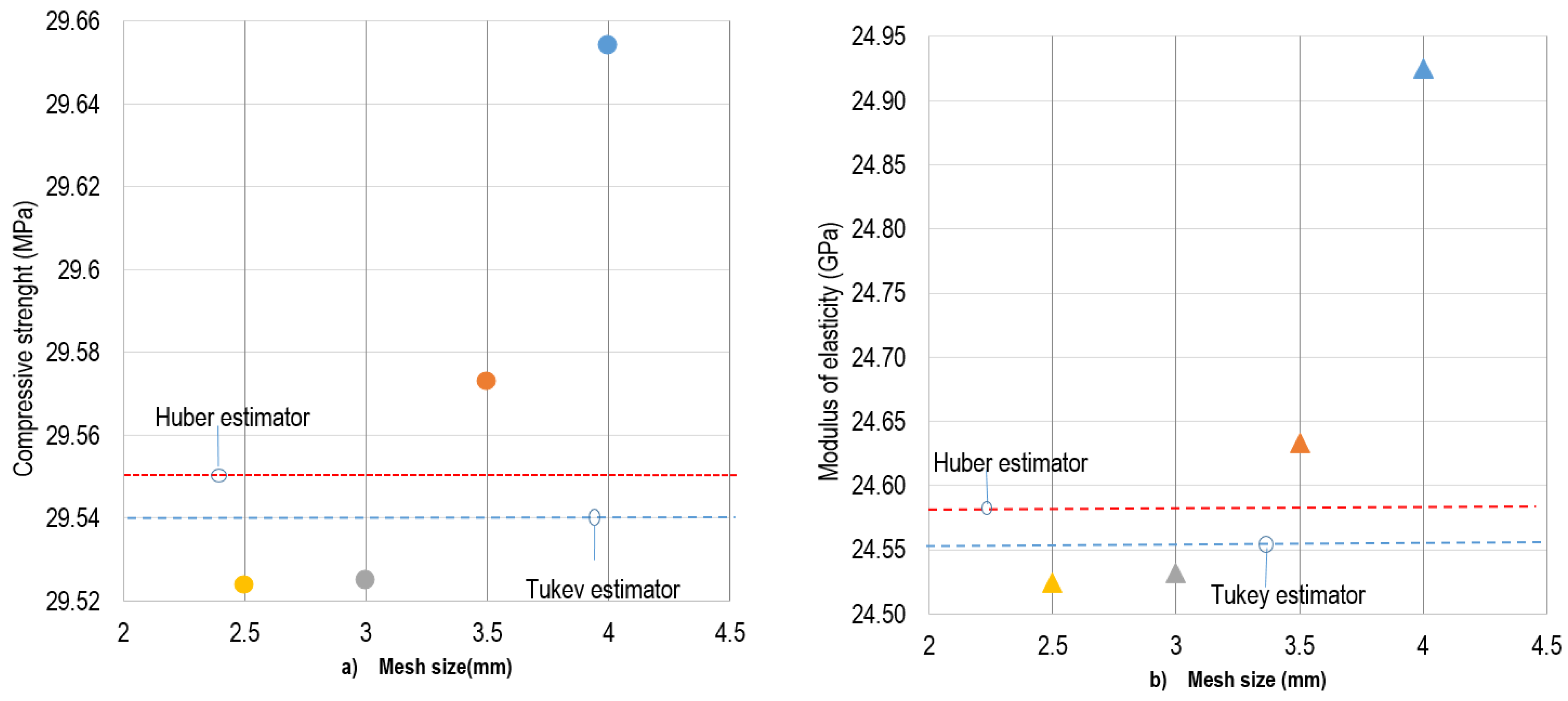
After assigning the properties of the materials obtained in the experimental model, simulations were developed with mesh sizes of 2.5, 3, 3.5, and 4.0 mm, respectively. Because the smallest coarse aggregate particle corresponded to the No. 4 sieve equivalent of 4.75 mm, it was assigned as the maximum mesh size of 4 mm.

Figure 5 contains the top view of the concrete cylinder; it was desired to show the differences in the mesh, where each quadrant of the associated view was assigned a different size. Each quadrant corresponded to a different mesh and showed an analogous way to appreciate the same effect of the meshing difference on the coarse aggregates. In a first stage, the test was carried out only elastically for each mesh size, where the elastic behavior was selected in Abaqus for both materials. In the second stage, the mechanical behavior was added with the help of the data about creep and plastic deformation, both in the coarse aggregate and in the mortar. The data was obtained in the experimental model, and the modeling was carried out until the failure of the cylinder.

3. Results

3.1. Experimental Model

The physical and mechanical properties determined for the materials used are listed in

Table 4. Basic properties of working materials.

Parameter	Test		Mortar	Coarse Aggregate
Modulus of elasticity	ASTM C39	GPa	20	43.6
Compressive strenght	ASTM C469	MPa	16.4	27-40
Unitary weight		KN/m3	21	22

. The results of the compression and elasticity tests are listed in

Table 5. Experimental results of compressive stress and modulus of elasticity.

Cylinder No.	Compressive Strength	Modulus of Elasticity
	MPa	GPa
1	28.63
2	28.71
3	28.81
4		23.42
5		23.62
6	28.73	23.56
Average	28.720	23.533

, and the yield zone data are listed in

Table 6. Characteristics of yielding on the experimental plastic zone.

Mortar		Coarse Aggregate
Yield Stress (MPa)	Plastic Strain	Yield Stress (MPa)	Plastic Strain
12.56	0	37.60	0.000000
15.64	0.0000077	40.54	0.000854
21.29	0.000008	45.20	0.000979
24.78	0.000044	50.07	0.001088
30.03	0.000051	55.29	0.001203
38.92	0.000154	60.35	0.001313
40.88	0.000267	65.11	0.001413
		70.30	0.001522
		75.62	0.001627
		80.14	0.001712

.

3.2. Computational Model

The geometry generated by the model needed to be very close to the experimental one, since the experimental model was required to serve as a comparison to the computational model. For this reason, the similarity between the previous gradations was essential for calibration.

Table 7. Data of gradations used.

Standard Sieve	Size (mm)	% Passing
		Referential	Experimental	Modeling
1″	25.4	100.000	100.000	100.000
3/4″	19.1	98.324	98.336	99.800
1/2″	12.7	64.804	65.049	61.500
3/8″	9.51	42.458	42.857	41.500
4	4.75	1.955	2.635	0.800

compares the granulometric values of the referential, the experimental, and the resulting granulometry in the modeling, showing a high precision between the results. On the other hand, Figure 6 shows us the granulometric curves used.

The modeling was carried out two times. In the first stage or moment, the behaviors of the materials were examined only in the elastic zone, for which the properties of unit weight and modulus of elasticity previously obtained in each of the materials were assigned. In this way, the results of maximum compressive stresses in the elastic zone and the respective elastic deformations were obtained for one of the simulations associated with mesh size, thus determining the modulus of elasticity E_c of the concrete.

Table 8. Characteristics of the elastic zone.

Parameter	4	3.5	3	2.5
Maximum elastic strength (MPa)	9.17	9.07	9.04	9.03
Elastic strain	0.0003679	0.0003682	0.0003685	0.0003682
Modulus of elasticity (GPa)	24.925	24.633	24.531	24.524

lists the individual numerical results associated with each mesh size, while Figure 7 shows the compression test curves for each mesh. Figure 8 shows the curves associated with each modeling by mesh size.

In the final part of the computational model, the plastic behavior was added to the elastic behavior previously worked on, for which it was necessary to add the characteristic data of the yield zone that corresponded to stresses and deformations in the plastic range for each material previously obtained in the test part. In this way, the cylinder was brought to failure in the way it was brought to failure experimentally; this way, it was possible to obtain the results of the maximum compressive strength by using the modeling associated with each mesh size used and graphically comparing them with the experimental value.

Table 9. Descriptive statistics.

	Mínimum Value	Maximum Value	Mean	Desv. Error	Deviation Standar
Compressive strength	29.52	29.65	29.5690	0.03055	0.06111
Modulus of elasticity	24.53	24.93	24.6538	0.09372	0.18744

presents the standard error values of the results, in which the error present in the results of the modulus of elasticity was three times greater than that generated in the compressive strength.

The experimental stress–strain curve in the elastic zone (up to a stress of approximately 9.3 MP) performed on cylinder No. 6 was listed and compared with the curves of the object from the model obtained in the first part of the modeling. Since the maximum unit strains were between 0.00035 and 0.0004, the values of the modulus of elasticity were very close to each other for the modeling and approximate if compared to the experimental value (Figure 9).

The increase in definition in the stress spectrum increased with decreasing mesh size. A cross-section in the main axis of the cylinder, exactly at the center of the cylinder, as shown in Figure 10, showed the sections in mesh sizes of 2.5 mm and 4.0 mm. They were facing each other to determine the difference in the intensity of efforts in the areas of interest. Some of the observations made were presented enclosed in dashed circles. They represented, among others, variations in the efforts and the precisions of areas with some specific effort.

The variations of results in the requested parameters were compared, with respect to the experimental values in

Table 10. Variation of the numerical results, compared to the experimental results.

Mesh Size mm	Variation(%)
	Compressive Strength	Modulus of Elasticity
4	3.150	5.91
3.5	2.877	4.67
3	2.715	4.24
2.5	2.711	4.21

. The differences in the 2.5 mm and 3 mm mesh were presented in the second decimal for the compression stress and in the second decimal for the modulus of elasticity.

M estimators were used as location and scale statistics for each research variable. Table 10 shows the Huber and Tukey estimators for the research variables. In Figure 11, next to the position of the results, these estimators were plotted.

Table 11. Statistical analysis with estimators M.

Parameter	Estimator M of Huber	Biweighted of Tukey
Compressive strength	29.5514	29.5418
Modulus of elasticity	24.5871	24.5636

contains the normal distances of each result with the two estimators. The smallest references were presented with the Turkey estimator in reference to the results of the 3 mm mesh (

Table 12. Statistical analysis with different mesh.

Mesh (mm)	Distance with Huber	Distance with Tukey	Distance with Huber	Distance with Tukey
4	0.103	0.112	0.338	0.362
3.5	0.022	0.031	0.046	0.070
3	0.026	0.017	0.055	0.032
2.5	0.027	0.018	0.062	0.039

), both for compressive strength and for modulus of elasticity.

4. Conclusions

The computational model managed to reproduce the compression test of concrete cylinders, with a good approach to the values of the experimental development in terms of gradation, compressive stress, and modulus of elasticity.

All assigned mesh sizes were close to each other and converged to the experimental value with some variations, depending on the assigned size. These differences appeared in different magnitudes in relation to the search event, such as compressive stress and elastic modulus.

Both at the level of compression and the modulus of elasticity, the mesh that offered the most functional result in terms of time and results was the 3.0 mm mesh. The results in mesh No. 2.5 only varied in the second decimal with respect to that of 3.0 mm, which was inefficient in terms of time. The review carried out with the Tukey estimator showed the 3.0 mm mesh to be the best performance result.

In terms of variation, the modulus of elasticity was more sensitive to variation in mesh size than compressive stress when using finite element analysis. The difference in results for the compressive stress was of the order of 3%, while for the modulus of elasticity, it was 4–6%. The error of the mean in the modulus of elasticity grew three times more than the resistance to compression, which established this parameter as more sensitive than the compressive strength.

Future research. Concrete modeling in its individual phases, in this case, coarse aggregate and mortar, allows us to give way to new possibilities by recreating different geometric shapes. For this, it is necessary to start modeling from known or referenced meshes.

References

1. Mehta, P.; Monteiro PJ, M. Concrete: Microstructure, Properties, and Materials; McGraw-Hill Education: New York, NY, USA, 2011. [Google Scholar]
2. Dos Santos, A.C.; de Arruda da Silva, T.J.; de Carvalho Palma Vitor, P.; Trautwein, L.M. Influence of coarse aggregate on concrete’s elasticity modulus. Acta Scientiarum. Technol. 2017, 19, 17–25. [Google Scholar] [CrossRef]
3. Piotrowska, E. Role of Coarse Aggregates in the Triaxial Behavior of Concrete: Experimental and Numerical Analysis. Ph.D. Thesis, Universite de Grenoble, Grenoble, France, 2013. [Google Scholar]
4. Zhou, F.; Lydon, F.; Barr, B. Effect of coarse aggregate on elastic modulus and compressive strength of high performance concrete. Cem. Concr. Res. 1995, 25, 177–186. [Google Scholar] [CrossRef]
5. Beshr, H.; Almusallam, A.A.; Maslehuddin, M. Effect of coarse aggregate quality on the mechanical properties of high strength concrete. Constr. Build. Mater. 2003, 17, 97. [Google Scholar] [CrossRef]
6. Tanesi, J.; Bentz, D.P.; Jones, S.Z.; Beyene, M.; Kim, M.; Ardani, A.; Arnold, J.; Stutzman, P.E. Influence of Aggregate Properties on Concrete Mechanical Performance. In Proceedings of the Transportation Research Board 96th Annual Meeting, Washington, DC, USA, 8–12 January 2017. [Google Scholar]
7. Vishalakshi, K.; Revathi, V.; Reddy, S.S. Effect of type of coarse aggregate on the strength properties and fracture energy of normal and high strength concrete. Eng. Fract. Mech. 2018, 194, 52–60. [Google Scholar] [CrossRef]
8. Piasta, W.; Góra, J.; Budzyński, W. Stress-strain relationships and modulus of elasticity of rocks and of ordinary and high performance concretes. Constr. Build. Mater. 2017, 153, 728–739. [Google Scholar] [CrossRef]
9. Walker, S.; Bloem, D.L. Effects of Aggregate Size on Properties of Concrete; National Sand and Gravel Association and National Ready Mixed Concrete Association: Washingtong, DC, USA, 1960. [Google Scholar]
10. Al-Oraimi, S.; Taha, R.; Hassan, H. The effect of the mineralogy of coarse aggregate on the mechanical properties of high-strength concrete. Constr. Build. Mater. 2005, 20, 499–503. [Google Scholar] [CrossRef]
11. Li, P.; Yu, Q.; Brouwers, H. Effect of coarse basalt aggregates on the properties of Ultra-high Performance Concrete (UHPC). Constr. Build. Mater. 2018, 170, 649–659. [Google Scholar] [CrossRef]
12. Akçaoğlu, T.; Tokyay, M.; Çelik, T. Effect of coarse aggregate size and matrix quality on ITZ and failure behavior of concrete under uniaxial compression. Cem. Concr. Compos. 2004, 26, 633–638. [Google Scholar] [CrossRef]
13. Meddah, M.S.; Zitouni, S.; Belâabes, S. Effect of content and particle size distribution of coarse aggregate on the compressive strength of concrete. Constr. Build. Mater. 2010, 24, 505–512. [Google Scholar] [CrossRef]
14. Sim, J.-I.; Yang, K.-H.; Jeon, J.-K. Influence of aggregate size on the compressive size effect according to different concrete types. Constr. Build. Mater. 2013, 44, 716–725. [Google Scholar] [CrossRef]
15. Li, M.; Hao, H.; Shi, Y.; Hao, Y. Specimen shape and size effects on the concrete compressive strength under static and dynamic tests. Constr. Build. Mater. 2018, 161, 84–93. [Google Scholar] [CrossRef]
16. Rashid, M.A.; Mansur, M.A.; Paramasivam, P. Correlations between Mechanical Properties of High-Strength Concrete. J. Mater. Civ. Eng. 2002, 14, 230–238. [Google Scholar] [CrossRef]
17. Lee, B.J.; Kee, S.-H.; Oh, T.; Kim, Y.-Y. Effect of Cylinder Size on the Modulus of Elasticity and Compressive Strength of Concrete from Static and Dynamic Tests. Adv. Mater. Sci. Eng. 2015, 2015, 580638. [Google Scholar] [CrossRef]
18. Araújo, S.S.; Guimarães, G.N.; Geyer, A.L.B.; Filho, A.C.; Sousa, J.L.A.D.O.E.; Filho, L.C.P.D.S.; Filho, R.D.T. Influence of the type of measuring device in determining the static modulus of elasticity of concrete. Rev. IBRACON de Estruturas e Mater. 2012, 5, 555–575. [Google Scholar] [CrossRef]
19. Gesoǧlu, M.; Güneyisi, E.; Özturan, T. Effects of end conditions on compressive strength and static elastic modulus of very high strength concrete. Cem. Concr. Res. 2002, 32, 1545–1550. [Google Scholar] [CrossRef]
20. Hunka, P.; Kolísko, J.; Vokáč, M.; Řeháček, S. Test and Technological Influences on Modulus of Elasticity of Concrete-Recapitulation. Procedia Eng. 2013, 65, 266–272. [Google Scholar] [CrossRef]
21. Suchánek, V.; Bednarz, T.; Svojanovský, T. Usage of Digital Image Correlation (DIC) in Determination of Modulus of Elasticity and Poisson’s Ratio of Special Concrete. Solid State Phenom. 2018, 272, 154–159. [Google Scholar] [CrossRef]
22. Huang, Y.; Liu, L.; Sham, F.; Chan, Y.; Ng, S. Optical strain gauge vs. traditional strain gauges for concrete elasticity modulus determination. Optik 2010, 121, 1635–1641. [Google Scholar] [CrossRef]
23. Maleki, M.; Rasoolan, I.; Khajehdezfuly, A.; Jivkov, A.P. On the effect of ITZ thickness in meso-scale models of concrete. Constr. Build. Mater. 2020, 258, 119639. [Google Scholar] [CrossRef]
24. Alañón, A.; Cerro-Prada, E.; Vázquez-Gallo, M.J.; Santos, A.P. Mesh size effect on finite-element modeling of blast-loaded reinforced concrete slab. Eng. Comput. 2017, 34, 649–658. [Google Scholar] [CrossRef]
25. Shishegaran, A.; Khalili, M.R.; Karami, B.; Rabczuk, T.; Shishegaran, A. Computational predictions for estimating the maximum deflection of reinforced concrete panels subjected to the blast load. Int. J. Impact Eng. 2020, 139, 103527. [Google Scholar] [CrossRef]
26. Azimi, M.; Mirjavadi, S.S.; Asli, S.A. Investigation of Mesh Sensitivity Influence to Determine Crack Characteristic by Finite Element Methods. J. Fail. Anal. Prev. 2016, 16, 506–512. [Google Scholar] [CrossRef]
27. González-Herrera, A.; Zapatero, J. Influence of minimum element size to determine crack closure stress by the finite element method. Eng. Fract. Mech. 2004, 72, 337–355. [Google Scholar] [CrossRef]
28. Wahid, N.; Stratford, T. Finite Element Modeling of Non-Loaded Reinforced Concrete One-Way Slab Exposed to Fire. ESTEEM Acad. J. 2022, 18, 11. [Google Scholar]
29. Guo, L.; Xiang, J.; Latham, J.-P.; Izzuddin, B. A numerical investigation of mesh sensitivity for a new three-dimensional fracture model within the combined finite-discrete element method. Eng. Fract. Mech. 2016, 151, 70–91. [Google Scholar] [CrossRef]
30. Mawlood, D.A.; Rafiq DS, K.; Adbullah, M.H. Nonlinear 3D Finite Element Model for Square Composite Columns Under Various Parameters. Iraqi J. Civ. Eng. 2022, 16, 10. [Google Scholar]
31. Breysse, D.; Balayssac, J.P. (Eds.) Non destructive in situ strength assessment of concrete. In Practical Application of Rilem TC249-ISC; Springer: Cham, Switzerland, 2022. [Google Scholar] [CrossRef]
Figure 1. Sequence of transformation activities: (a) original rocks of limestones, (b) cutting cores for mechanical and elastic tests, (c) laminar cutting of rock, (d) spherical shaping of particles, and (e) grouping of shaped particles to make a cylinder of 100 mm × 200 mm.
Applsci 13 02352 g001
Figure 2. Comparison between reference and experimental gradations for spherical particles.
Applsci 13 02352 g002
Figure 3. Sequence of final activities: (a) mixing of materials, (b) conformation of concrete cylinders, and (c) elastic modulus test.
Applsci 13 02352 g003
Figure 4. Phases in the model: (a) spatial distribution of the phase of spherical particles. (b) Mortar phase. (c) Vertical sectional view of the aggregates. (d) Vertical sectional view of the mortar.
Applsci 13 02352 g004
Figure 5. Different mesh sizes used. (left) Top view of the cylinder. (right) Top view of the coarse aggregate particles.
Applsci 13 02352 g005
Figure 6. Granulometric curves used.
Applsci 13 02352 g006
Figure 7. Modeling results vs. experimental value. Modulus of elasticity.
Applsci 13 02352 g007
Figure 8. Modeling results vs. experimental value. Compressive strength.
Applsci 13 02352 g008
Figure 9. Compression curves in the elastic zone for each mesh size.
Applsci 13 02352 g009
Figure 10. Sections generated by cross-section at the center of the cylinder. (a) 2.5 mm mesh, (b) 4 mm mesh.
Applsci 13 02352 g010
Figure 11. Statistical analysis with M estimators. (a) Applied on compressive strength. (b) Applied on modulus of elasticity.
Applsci 13 02352 g011