Reversible Image Processing for Color Images with Flexible Control

Abstract

In this paper, we propose an image processing method for color images to reversibly achieve flexible functions. Most previous research has focused on reversible contrast enhancement (CE) for grayscale images. When we directly apply these methods to color images, hue distortion is caused. Several previous methods have been proposed for color images. These methods, however, only have a CE function. We previously proposed a reversible method for color images that enhances the brightness contrast and improves the saturation. Without losing the advantages of our previous method, we propose a new method to expand the ability of image processing. The proposed method reversibly achieves not only CE and saturation improvement but also sharpening or smoothing and brightness increases or decreases. It ensures full reversibility and thus perfectly reconstructs raw images in any case. The experimental results demonstrate the effectiveness of the proposed method in terms of image quality and reversibility.

1. Introduction

Recently, we widely use image processing applications to obtain desired images. These techniques, however, do not ensure reversibility. If we aim to recover a raw image, then the raw image itself or editing information is required in addition to the processed image (hereafter the output image). This problem notably affects devices with a limited storage capacity, such as smartphones and laptops. Furthermore, in fields for particular types of images such as medical, military, and satellite images, it is essential to perfectly restore raw images. Thus, reversible image processing techniques have been actively researched to recover raw images without increasing the image’s data amount. Specifically, reversible contrast enhancement (CE) [1,2,3,4,5,6,7,8,9,10,11,12,13] methods have been proposed. They have been commonly researched for images with uncompressed formats such as tiff, bmp, and pgm or ppm. These methods guarantee reversibility by using reversible data hiding (RDH) techniques.

Data hiding techniques have been studied to detect malicious alterations in images and prevent unauthorized use of images [14,15]. They are classified as two types: irreversible and reversible. The former has accomplished high resistance against attacks and a high hiding capacity. However, it can never restore raw images, even after data extraction. On the other hand, the latter is generally vulnerable against attacks and has a relatively low hiding capacity, while raw images can be perfectly recovered after data extraction. The above reversible CE methods are based on the latter technique and can reconstruct raw images by embedding recovery information into the images.

Most of the reversible CE methods [1,2,3,4,5,6,7,8,9,10] have been investigated for eight-bit grayscale images. Multiple methods [1,2,3,4,5] were proposed for natural images to refine the CE effect, while some other methods [6,7,8] focused on medical images. On another front, the methods developed by the authors of [9,10] had an automatic CE function without manually controlling complex parameters. When these methods are directly applied to color images, perceptible hue distortion arises. Additionally, there are few methods specifically for color images. Nevertheless, two previous methods [11,12] have been proposed to tackle this problem. These methods execute the CE function for color images but still cause hue distortion or cannot ensure reversibility. Furthermore, they perform only the CE function, and other functions have not been considered. Note that the bit depth of their target color images is 24 bits.

To attain an extra function, we previously proposed a reversible image processing method for color images [13] that is based on the method in [12]. It achieves CE and saturation improvement independently. To ensure reversibility, it embeds the recovery information by using an RDH method.

In this paper, we propose a novel image processing method for color images with perfect reversibility. The proposed method enables flexible control for brightness (i.e., sharpening, smoothing, increasing, decreasing, and CE). Additionally, the saturation can be selectively improved. This method is an extension of our previous method [13] and preserves its advantages. Through our experiments, we verify the availability of the proposed method from the standpoints of image quality and reversibility.

The rest of this paper is organized as follows. In Section 2, we describe the related works and background information to facilitate understanding of the proposed method. In Section 3, we propose a new reversible image processing method. The experimental results demonstrate the performance of the proposed method in Section 4. Finally, we conclude this paper in Section 5.

2. Related Works

2.1. Contrast Enhancement Methods for Grayscale Images

Reversible CE methods [1,2,3,4,5,6,7,8,9,10] have been widely researched for grayscale images. Their main purpose is to reversibly enhance the contrast without increasing the data amount for each image. Reversible CE methods perfectly reconstruct raw images by using RDH techniques.

Wu et al. [1] designed a reversible CE method for grayscale images by using a histogram shifting (HS)-based RDH technique. This method embeds recovery information into an image histogram, and the raw images are perfectly restored. On the basis of this fundamental method, many extended approaches have been published [2,3,4,5,6,7,8,9,10] in which the CE function is refined in terms of local contrast, output image quality, CE effect, application to medical images, automation, or brightness preservation. The local contrast was improved by Jafar et al. [2]. In their method, k-means clustering is conducted by using the correlation among each pixel and its three neighboring pixels. Zhang et al. [3] built upon Jafar et al.’s method [2] to improve the effectiveness of k-means clustering. Their method refers to four neighboring pixels for each pixel and considers the correlation among them using multiple elements, such as the variance, mean, and median. Wu et al. [4] modified the preprocessing of the CE function [1]. This method prevents perceptual distortion caused by preprocessing, so the output images have a high image quality. To refine the CE effect, a two-dimensional image histogram was used by Wu et al. [5]. Their method can obtain the correlation among pixels with higher accuracy and provide more effective CE. For medical images, several CE methods [6,7,8] have been proposed. These methods first apply a region segmentation process to a raw image and divide the image into regions of interest (ROIs) and non-ROIs. The CE function is subsequently executed on the ROIs only. Kim et al. [9] developed an automatic CE method. Their method automatically repeats the CE function until the amount of recovery information exceeds the hiding capacity. The automatic CE method, however, causes an excessive enhancement effect and cannot preserve the brightness. To improve the performance of this method, an extended method [10] was designed. Their method optimally defines the direction in which to shift the image histogram in each HS sequence so as to maintain the mean of the brightness. Additionally, when the CE function excessively changes the brightness, their method breaks the repetition process. Consequently, this method can preserve the brightness and prevent the excessive enhancement effect.

The above CE methods are designed for grayscale images. If these methods are applied to color images, then hue distortion occurs. To tackle this issue, several CE methods [11,12] have been considered for color images.

2.2. Contrast Enhancement Methods for Color Images

To enhance the contrast without hue distortion, effective methods have been proposed for color images [11,12]. A reversible CE method for color images [11] was published that combines the advantages of previous methods [5,10]. This method applies a single reversible CE algorithm to the R, G, and B components independently, and raw images are perfectly restored. This method not only preserves the brightness but also refines the CE effect. However, hue distortion is still caused. Wu et al. [12] designed another method by using the HSV color space. Their method enhances the brightness contrast, which is simply referred to as contrast hereafter, without saturation or hue distortion. However, rounding errors arise in the preservation functions for the saturation and hue. The restored images have a high image quality, but raw images cannot be fully reconstructed.

These previous methods [11,12] can carry out the CE function on color images. Nevertheless, they only focus on the CE function, and other functions have not been considered. We previously proposed a reversible method [13] for color images based on the method in [12] to not only enhance the contrast but also improve the saturation.

2.3. Contrast Enhancement and Saturation Improvement Method for Color Images

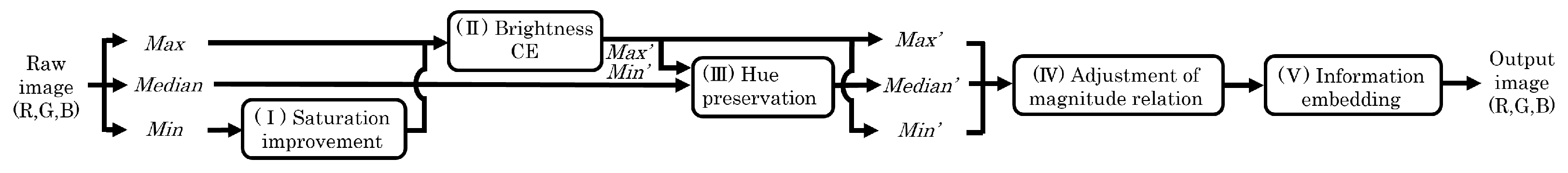
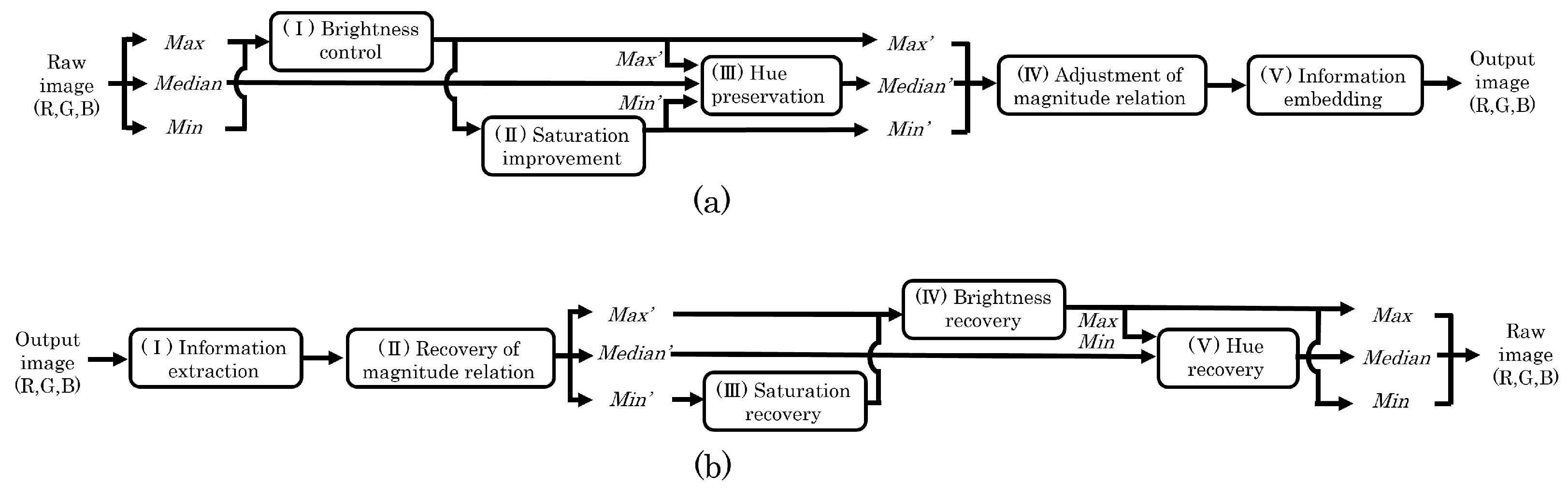
Our previously proposed method [13] for color images based on [12] enables CE and saturation improvement independently. Additionally, perfect reversibility can be ensured by embedding recovery information.

This method uses the HSV color space to enable both CE and saturation improvement functions without hue distortion. The HSV color space consists of the hue (H), saturation (S), and brightness (V). The color space is classified under two types: the cylinder model [16] and cone model [17,18]. The HSV components are generally given by

$$H=\left\{\begin{array}{cc}60\times \frac{G-B}{Max-Min}\hfill & \mathrm{if}Max=R\hfill \\ 60\times (\frac{B-R}{Max-Min}+2)\hfill & \mathrm{if}Max=G\hfill \\ 60\times (\frac{R-G}{Max-Min}+4)\hfill & \mathrm{if}Max=B\hfill \\ notdefined\hfill & \mathrm{if}Max=0,\hfill \end{array}\right.$$

(1)

$$S_{cylinder}=\left\{\begin{array}{cc}\frac{Max-Min}{Max}\hfill & \mathrm{if}Max\ne 0\hfill \\ 0\hfill & \mathrm{if}Max=0,\hfill \end{array}\right.$$

(2)

$$S_{cone}=Max-Min,$$

(3)

$$V=Max,$$

(4)

where $Max$, $Median$, and $Min$ indicate the largest, middle, and smallest values in the RGB components, respectively. Note that the above variables are used as matrices in this paper. The method in [12] uses the cylinder model, where the saturation has fractional values with Equation (2). Thus, rounding errors arise by controlling the saturation. In comparison, our previous method uses the cone model. Since the saturation has integer values in the cone model with Equation (3), this method can reversibly improve the saturation without rounding errors.

We give an outline of our previous method in Figure 1. The largest, middle, and smallest values in the R, G, and B components of each pixels are assigned to $Max$, $Median$, and $Min$, respectively. First, the saturation is improved by decreasing the $Min$ values (see Figure 1(I)). In the case that we would not like to improve the saturation, this function can be skipped. The contrast is then enhanced by applying the HS method [1] to the $Max$ values (see Figure 1(II)). Next, we adjust the $Median$ values to avoid hue distortion (see Figure 1(III)). The $Ma{x}^{\prime }$, $Media{n}^{\prime }$, and $Mi{n}^{\prime }$ values are further calibrated to maintain the magnitude relation among RGB components and turned back into R, G, and B values, respectively (see Figure 1(IV)). Finally, the recovery information, which is used to restore the raw image, is embedded into each color component by the prediction error expansion with histogram shifting (PEE-HS) method [19] (see Figure 1(V)). Accordingly, our previous method can conduct CE and saturation improvement reversibly and independently.

Note that color space conversion from RGB to HSV is not used in this method. If a series of processes is applied in the HSV color space, then a number of rounding errors arise through the color space conversion. These rounding errors prevent us from perfectly recovering the raw images. Thus, the H, S, and V values are indirectly controlled using the $Max$, $Median$, and $Min$, and all functions in our previous method are practically carried out in the RGB color space.

In the next section, we propose a novel reversible processing method for color images based on our previous method. The proposed method features both a sharpening and smoothing function and brightness increase and decrease function, along with the advantages of our previous method.

3. Proposed Method

We propose an image processing method for color images with perfect reversibility and multiple functions. As described in the former section, the previous methods focused only on the CE function, so other functions were not considered. In comparison, the proposed method enables a sharpening and smoothing function and brightness increase and decrease function. The method can also perform CE and saturation improvement, which are the advantages of our previous method [13]. In the proposed method, all the functions can be carried out independently from each other. In comparison, several functions can be applied to an image simultaneously. Specifically, we can choose one or two types of brightness controls and saturation improvement. We describe the procedures for image processing and raw image recovery in detail as follows.

3.1. Image Processing

Here, we explain the outline of image processing in Figure 2a. We can select one or two types of functions from among five brightness controls: sharpening and smoothing, brightness increase and decrease, and CE functions. Here, our method can carry out two types of brightness controls simultaneously.

The largest, middle, and smallest values in the R, G, and B components of each pixel are assigned to $Max$, $Median$, and $Min$, respectively. We regulate the $Max$ and $Min$ values so as to use the selected brightness controls (see Figure 2a(I)). Depending on the user’s intention, the saturation is subsequently improved (see Figure 2a(II)). The $Median$ value is then adjusted to avoid hue distortion (see Figure 2a(III)). The $Ma{x}^{\prime }$, $Media{n}^{\prime }$, and $Mi{n}^{\prime }$ values are further calibrated to maintain the magnitude relation among RGB components and turned back into R, G, and B values, respectively (see Figure 2a(IV)). Recovery information is finally embedded into each color component by using the PEE-HS method [19] (see Figure 2a(V)). Accordingly, our new method can reversibly control the brightness and improve the saturation.

As described above, our proposed method can conduct one or two functions for brightness from five control types: sharpening and smoothing, brightness increase and decrease, and CE functions. It also performs brightness control and saturation improvement independently. The recovery information is required for each function. In the case where the number of functions is increased, the amount of recovery information is accumulated and might exceed the hiding capacity. In such a case, reversibility cannot be fully ensured. Through our experiments, reversibility was constantly ensured under the combination of up to two types of brightness controls and saturation improvement. We separately explain the sharpening and smoothing function, the brightness increase and decrease function, and how to guarantee reversibility.

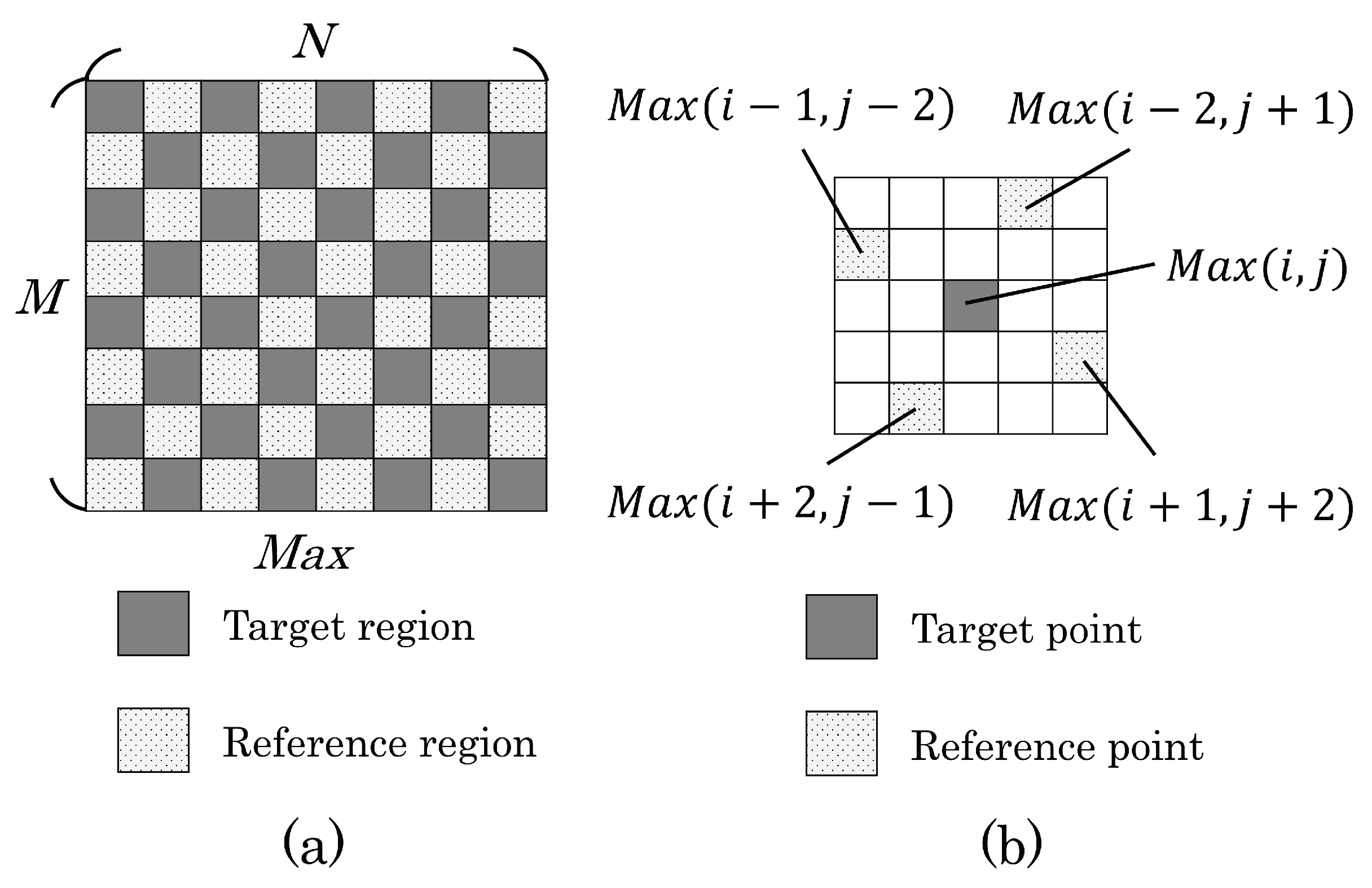
3.1.1. Sharpening and Smoothing

As shown in Figure 3a, the $Max$ values are divided into target and reference regions in a checkered pattern. We define each $Max$ value in the target and reference regions as target or reference points, respectively. Our method carries out the sharpening or smoothing function for each target point by using four reference points. Figure 3b shows the relationship among the target and adjacent points. We give details on the procedure below:

Step 1:

Divide the $Max$ values into the target and reference regions.

Step 2:

Apply Equation (5) for sharpening or Equation (6) for smoothing to each target point:

$$\begin{array}{cc}\hfill Ma{x}^{\prime }(i,j)& =round[2\times Max(i,j)-\frac{1}{5}\times \{Max(i-2,j+1)\hfill \\ \hfill & +Max(i-1,j-2)+Max(i,j)\hfill \\ \hfill & +Max(i+2,j-1)+Max(i+1,j+2)\left\}\right],\hfill \end{array}$$

(5)

$$\begin{array}{cc}\hfill Ma{x}^{\prime }(i,j)& =round[\frac{1}{5}\times \{Max(i-2,j+1)+Max(i-1,j-2)\hfill \\ \hfill & +Max(i,j)+Max(i+2,j-1)+Max(i+1,j+2)\left\}\right].\hfill \end{array}$$

(6)

Given an image with a size of $M\times N$, $Max(i,j)$ and $Ma{x}^{\prime }(i,j)$ denote the original and output target points, respectively. $Max(i-2,j+1)$, $Max(i-1,j-2)$, $Max(i+2,j-1)$, and $Max(i+1,j+2)$ represent the four reference points, where $3\le i\le M-2$ and $3\le j\le N-2$.

Step 3:

Obtain $Mi{n}^{\prime }$ with the following equation on the basis of Equation (3):

$$Mi{n}^{\prime }=Ma{x}^{\prime }-S_{cone}.$$

(7)

This step prevents saturation distortion.

The proposed method rounds the fractional parts of $Max$. Another type of error due to underflows (UFs) might be caused for $Mi{n}^{\prime }$ by Equation (7). Such errors prevent the raw image from being recovered. Therefore, our method preserves the errors as recovery information. We will elaborate on this in Section 3.1.3.

Depending on the user’s intention, the above procedure can be repeated by exchanging the target and reference regions. The proposed method can iterate a series of the above steps until the amount of the recovery information exceeds the capacity of the embedding process. We define the number of processing times for sharpening and smoothing as $I_{VSH}$ and $I_{VSM}$, respectively. These parameters enable us to control the degree of effect of these functions.

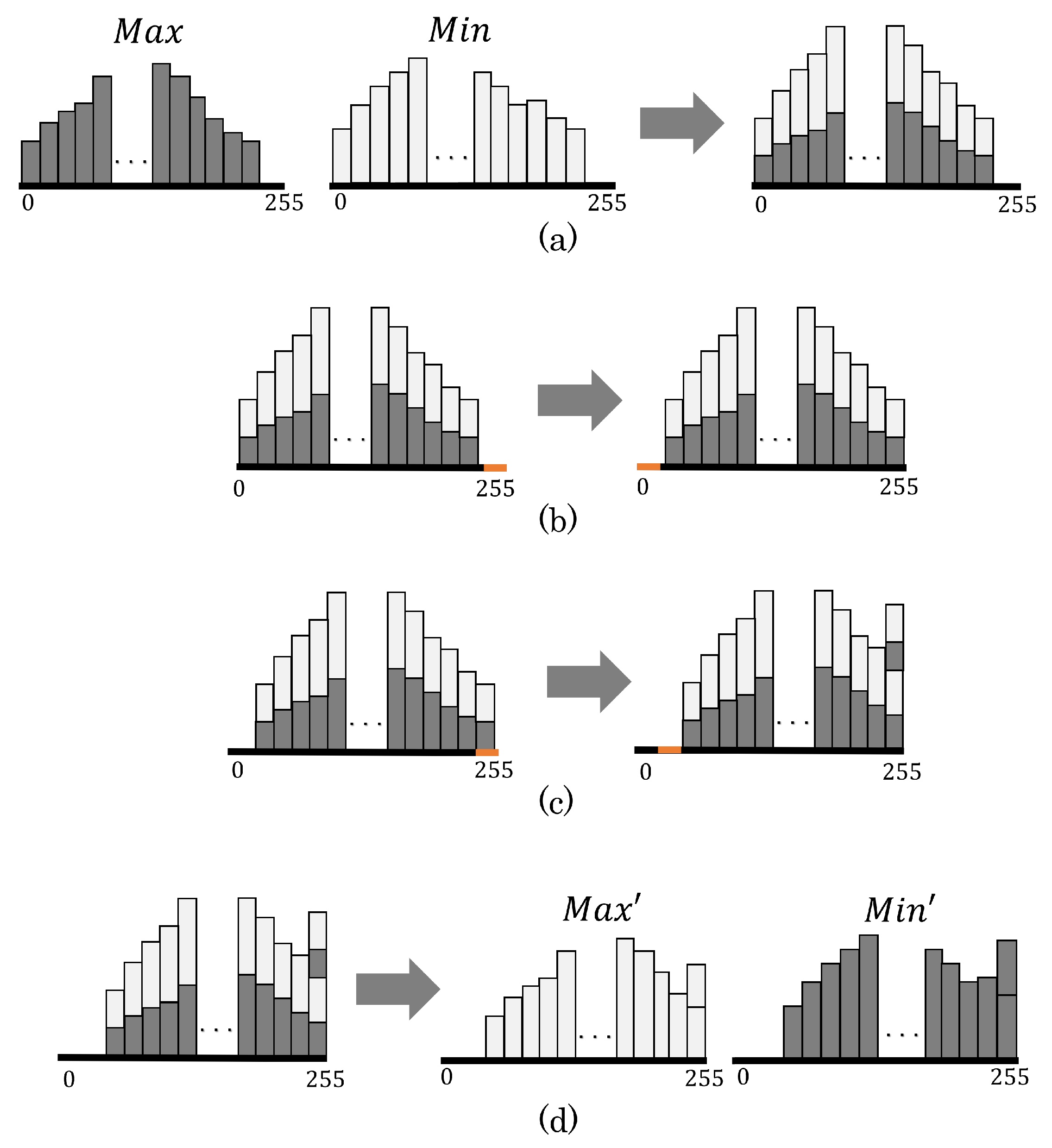
3.1.2. Brightness Increase or Decrease

The proposed method can increase or decrease the brightness by shifting the integrated histograms of $Max$ and $Min$. The integrated histogram is essential for the proposed method so as to ensure that the magnitude relation is invariant before and after the shifting process. In the practical implementation, our method concatenates the $Max$ and $Min$ matrices to obtain the integrated histogram while splitting the concatenated matrix into the $Max’$ and $Min’$ ones. We will first describe the brightness increase function:

Step 1:

Integrate the histograms of $Max$ and $Min$ (see Figure 4a).

Step 2:

Define the rightmost bin of the histogram as the reference bin. In the case where the number of pixels belonging to the reference bin exceeds 1% of the total number of pixels, the left adjacent bin is alternatively defined as the reference bin.

Step 3:

Shift the pixels contained in the bins between the reference and the leftmost ones by +1 (see Figure 4b,c). In the case where the reference bin is not empty, the pixels in the reference and left adjacent bins are superimposed (see Figure 4c).

Step 4:

Separate the integrated histogram into the $Ma{x}^{\prime }$ and $Mi{n}^{\prime }$ ones (see Figure 4d).

In comparison, in the brightness decrease function, the leftmost bin is defined as the reference bin in Step 2, and the pixels belonging to the bins between the reference and rightmost ones are shifted by −1 in Step 3. Here, the threshold of 1% in Step 2 is the optimal parameter determined through our experiments. By introducing this parameter, the proposed method can automatically select a bin with a small number of pixels as a reference bin. The reference bin will be merged with the adjacent bin. This leads to the reduction of the amount of recovery information. We define the numbers of processing times for a brightness increase or decrease as $I_{VI}$ and $I_{VD}$, respectively. These parameters enable us to control the degree of effect of these functions. We will give details on the essential information for the recovery process in Section 3.1.3.

3.1.3. Recovery Information

The proposed method embeds the recovery information to restore raw images. Three-bit data are first required to distinguish the five types of brightness controls: sharpening, smoothing, increase, decrease, and CE. One-bit data are further used to verify the numbers of the brightness controls to be conducted. This method can apply one or two functions for the brightness. When the CE function is selected, the other recovery information is the same as in the previous method [13]; otherwise, we need the following information:

(i)

For Sharpening and Smoothing

As described in Section 3.1.1, the sharpening and smoothing functions cause rounding errors in the $Ma{x}^{\prime }$ and $Mi{n}^{\prime }$ vlaues. These errors prevent us from restoring the raw images. Thus, we need to record the rounding errors as recovery information. If a large number of rounding errors arises, then the amount of recovery information may exceed the hiding capacity. Two location maps are prepared for $Max$ and $Min$ to store the pixels with rounding errors. Our method compresses the maps and error values according to the JBIG2 standard [20] and Huffman coding, respectively. The above data are required for every single process. Additionally, the parameter values of $I_{VSH}$ or $I_{VSM}$ should be stored for reversibility.

(ii)

For Brightness Increase or Decrease

The bin data before image processing (hereafter the intact bin data) need to be stored. The intact bin data mainly consist of three types of data. The first is the eight-bit pixel value of the reference bin in Step 2. The second is the one-bit classification data for distinguishing whether the reference bin is empty or not in Step 3. In the case where the reference bin is not empty, extra one-bit data are essential for each integrated pixel to discriminate the original bin, namely the reference or adjacent bin. The above data are required for every single process.

The recovery information is embedded into the RGB components in the final step. In this paper, we use the PEE-HS method [19], which is one of the most typical methods in this area. The PEE-HS method can hide information in a prediction error histogram with the minimum perceptional distortion, so many extended methods have been proposed based on it. Note that we can use another RDH method on behalf of this method.

To reduce the amount of recovery information, we further modified the preprocessing of an efficient RDH method [4] and introduced the extended one into our method. Here, the preprocessing is conducted on the integrated histogram of the R, G, and B components to restrain the hue distortion. In contrast, a PEE-HS method is applied to RGB components independently.

3.2. Raw Image Recovery

Figure 2b illustrates a block diagram of the recovery process. The recovery information is extracted from each color component (see Figure 2b(I)). The largest, middle, and smallest values in the R, G, and B components of each pixel are assigned to $Ma{x}^{\prime }$, $Media{n}^{\prime }$, and $Mi{n}^{\prime }$, respectively. Then, the original magnitude relation is recovered (see Figure 2b(II)). If the saturation has been improved, then the original saturation is recovered (see Figure 2b(III)). The type of brightness control is identified with the recovery information, and we can restore $Max$ and $Min$ through the recovery process (see Figure 2b(IV)). In the case where two types of brightness controls have been applied, the recovery process for the latter one should be carried out first. The hue is subsequently restored, and the $Median$ value is recovered (see Figure 2b(V)). Finally, $Max$, $Median$, and $Min$ are turned back into R, G, and B values, respectively. Accordingly, our new method can perfectly reconstruct the raw image. We will elaborate on the way we retrieve the raw image for each function.

3.2.1. Recovery from Sharpening and Smoothing

The proposed method retrieves raw images from the sharpening or smoothing function by using the information described in Section 3.1.3(i). The recovery process consists of three steps:

Step 1:

Divide $Ma{x}^{\prime }$ into target and reference regions, similar to with $Max$ in Step 1 of Section 3.1.1.

Step 2:

Restore the original of each target point by using Equation (5) for sharpening or Equation (6) for smoothing. Accordingly, $Max$ is recovered.

Step 3:

Restore $Min$ from $Mi{n}^{\prime }$ by using Equations (3) and (7).

When errors are caused by rounding or UF for $Ma{x}^{\prime }$ or $Mi{n}^{\prime }$, these errors are modified by the recovery information. Additionally, in the case where the sharpening or smoothing function has been repeated in Section 3.1.1, $Max$ and $Min$ are restored by the recovery process $I_{VSH}$ or $I_{VSM}$ times, respectively.

3.2.2. Recovery from Brightness Increase or Decrease

The proposed method recovers raw images from the brightness increase or decrease function by using the information described in Section 3.1.3(ii). We first describe the procedure for the brightness increase function:

Step 1:

Integrate the histograms of $Ma{x}^{\prime }$ and $Mi{n}^{\prime }$.

Step 2:

Obtain the reference bin value and the classification data, which indicate whether the reference bin was empty or not before the increasing process, from the recovery information.

Step 3:

Shift the pixels belonging to the bins between the reference and leftmost ones by −1. In the case where the reference bin was not empty before the increasing process, the pixels, which have been integrated in the left adjacent bin, are turned back to the reference bin by referring to the recovery information. Accordingly, the original values of $Max$ and $Min$ are recovered.

Step 4:

Separate the integrated histogram into $Max$ and $Min$ histograms.

$Max$ and $Min$ are recovered by the above processes $I_{VI}$ times. For the recovery process for the brightness decrease function, the pixels belonging to the bins between the reference and rightmost ones are shifted by +1 in Step 3, and the number of processing times will be $I_{VD}$.

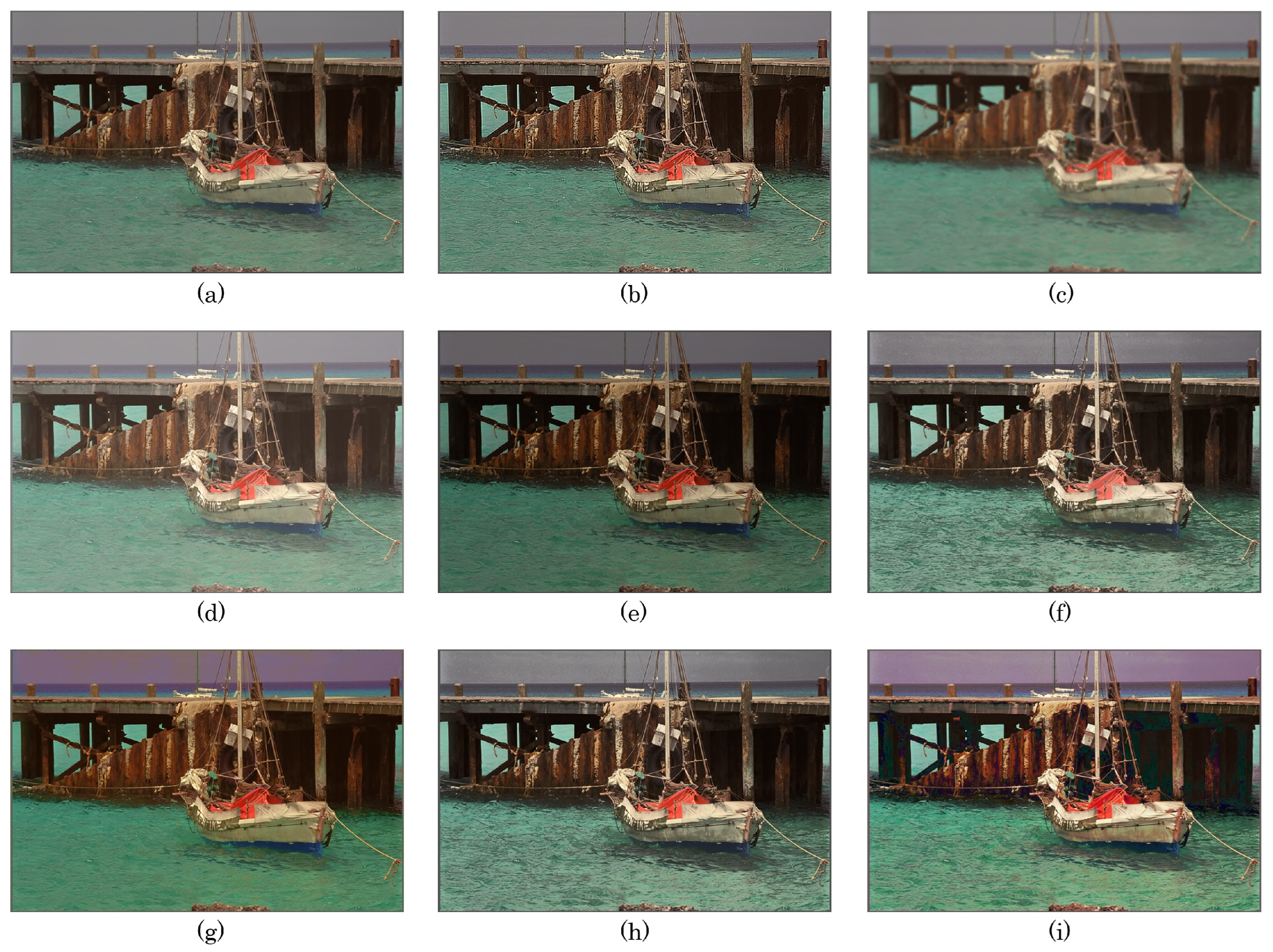
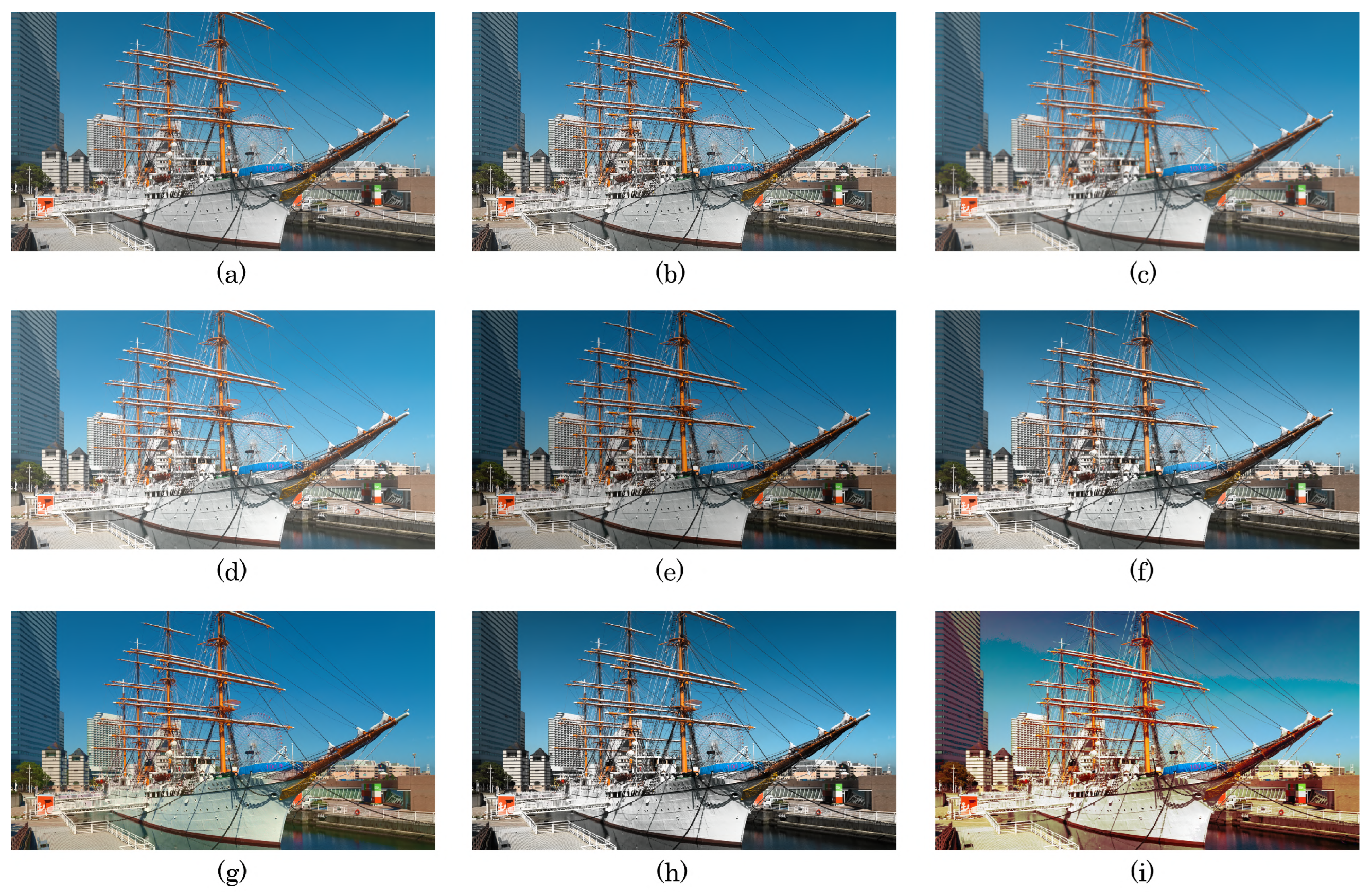
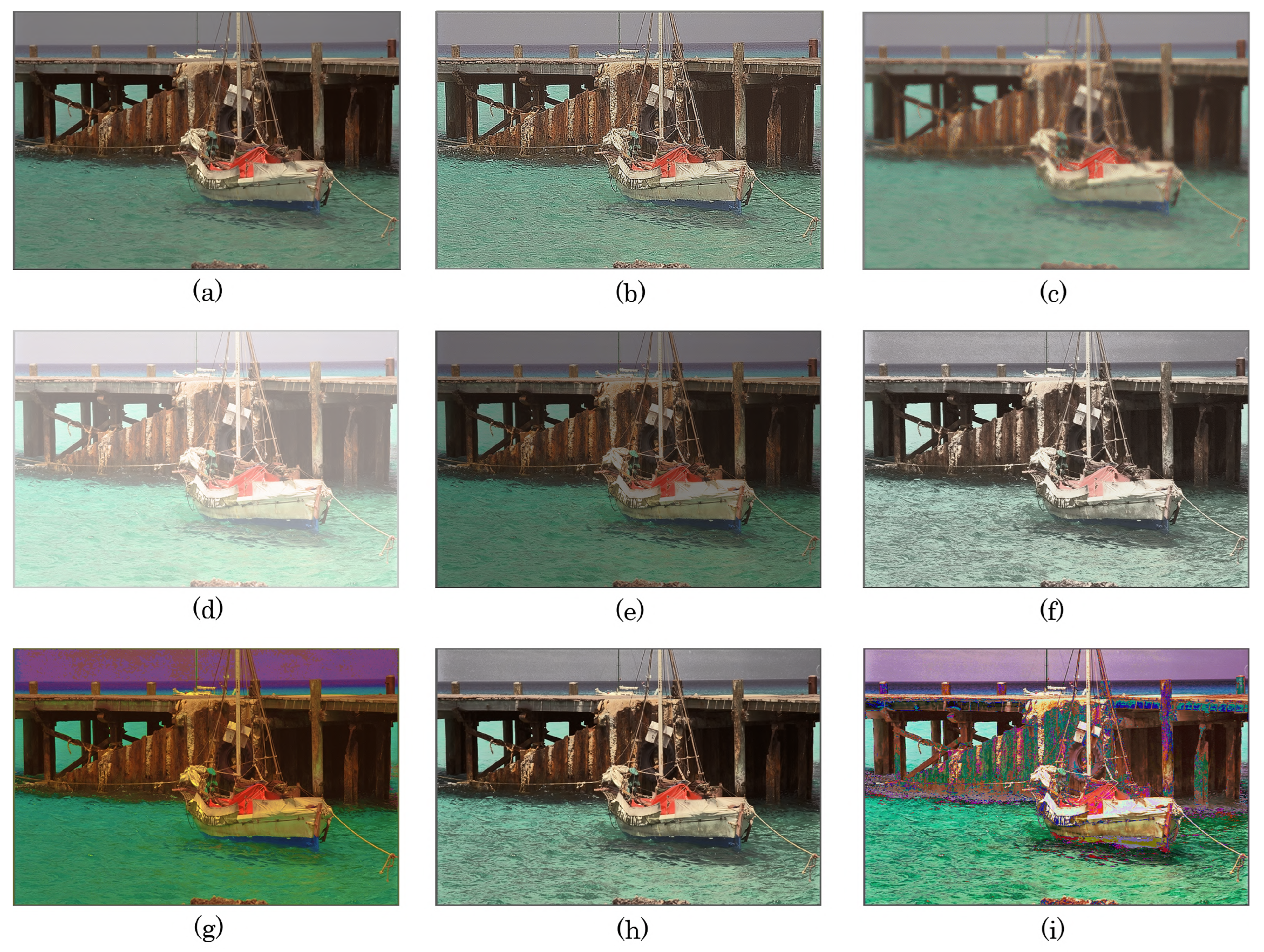
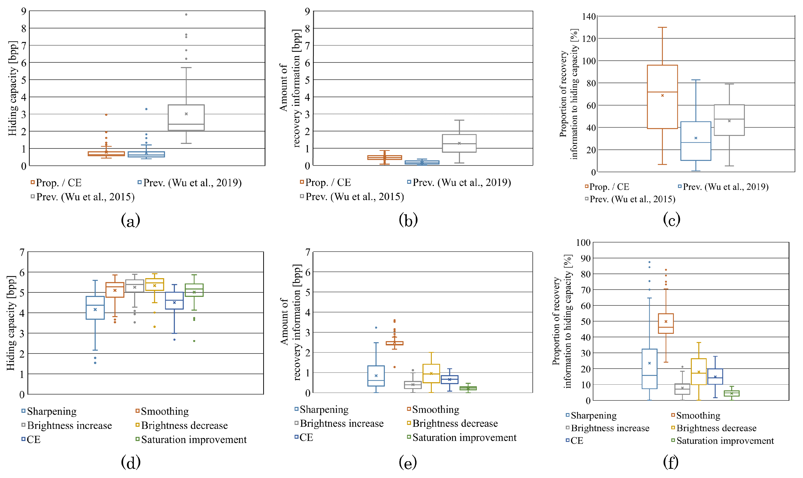
4. Experimental Results

We assessed the output images derived with the proposed method and the previous methods [1,12] from the perspectives of image quality and reversibility. In the experiments, 64 color images were used from five databases [21,22,23,24,25].

Table 1. Test images.

Database	# of Images	Image Size
Kodak [21]	24	768 × 512
SIPI [22]	6	512 × 512
McMaster [23]	18	500 × 500
IHC [24]	6	4608 × 3456
ITE [25]	10	1920 × 1080 (converted from bit depth of 48 to 24)

gives the details on the test images. The target format of the proposed method is the 24 bit depth color image. Thus, the test images of the ITE database were converted from a bit depth of 48 to 24 so as to have an identical bit depth with those of the other databases. Note that $I_{VSH}$, $I_{VSM}$, $I_{VI}$, $I_{VD}$, $I_{VC}$, and $I_S$ represent the number of processing times for sharpening and smoothing, brightness increase and decrease, CE, and saturation improvement, respectively.

The rest of this section is organized as follows. Section 4.1 gives details on the evaluation indices. In Section 4.2, we confirm the effectiveness of the brightness control, saturation improvement, and hue preservation for the proposed method. With respect to the CE function, we compare the output images derived by the proposed method and previous methods. The images output with the maximum level of each function are assessed in Section 4.3. Section 4.4 presents an evaluation on reversibility. The performance of the embedding process is evaluated in Section 4.5. In Section 4.6, we further verify the effectiveness of coregulation with multiple functions in the proposed method.

4.1. Evaluation Indices

Multiple types of evaluation indices are used in the following subsections. First, we assessed the levels of sharpening and smoothing through the difference in standard deviations between the raw and output images. For the brightness increase or decrease levels, the brightness difference was used. We explored the CE level with the relative contrast error (RCE) [26]:

$$RCE=0.5+\frac{st{d}_{V^{\prime }}-st{d}_V}{255},$$

(8)

where $st{d}_V$ and $st{d}_{V^{\prime }}$ denote the standard deviations of the brightness for the raw and output images, respectively. The RCE value ranges from 0 to 1. When the contrast is enhanced from a raw image, the RCE value exceeds 0.5. In regard to the saturation improvement level, the saturation difference was calculated. Hue preservation was further confirmed by the absolute hue difference. To verify reversibility, the quality of the restored images was assessed by using PSNR, SSIM [27], and CIEDE2000 [28].

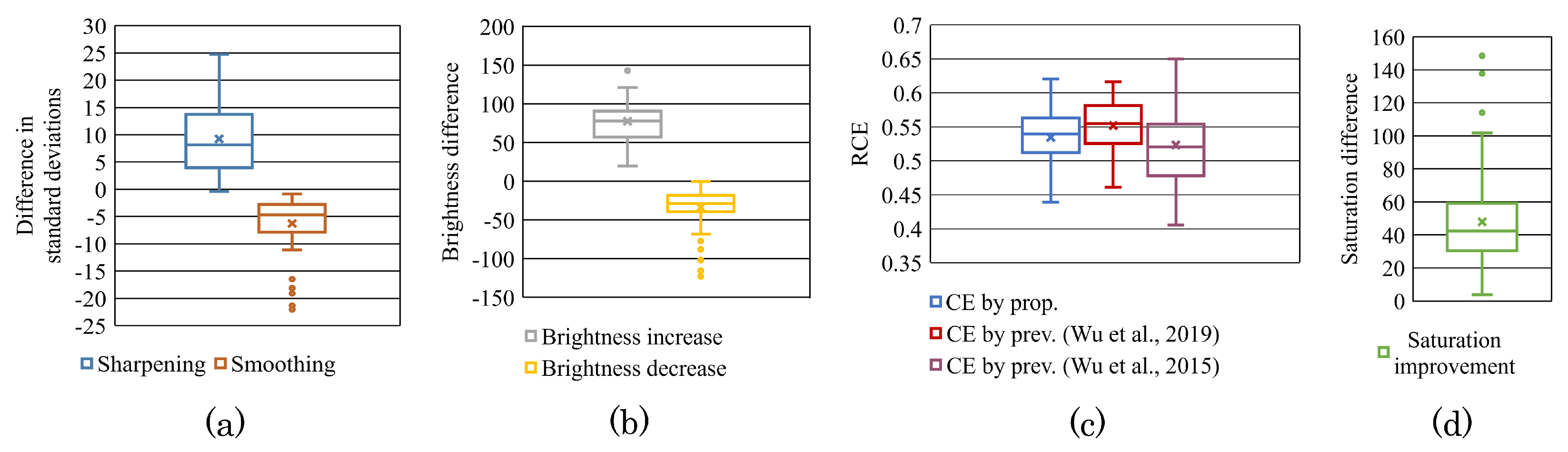
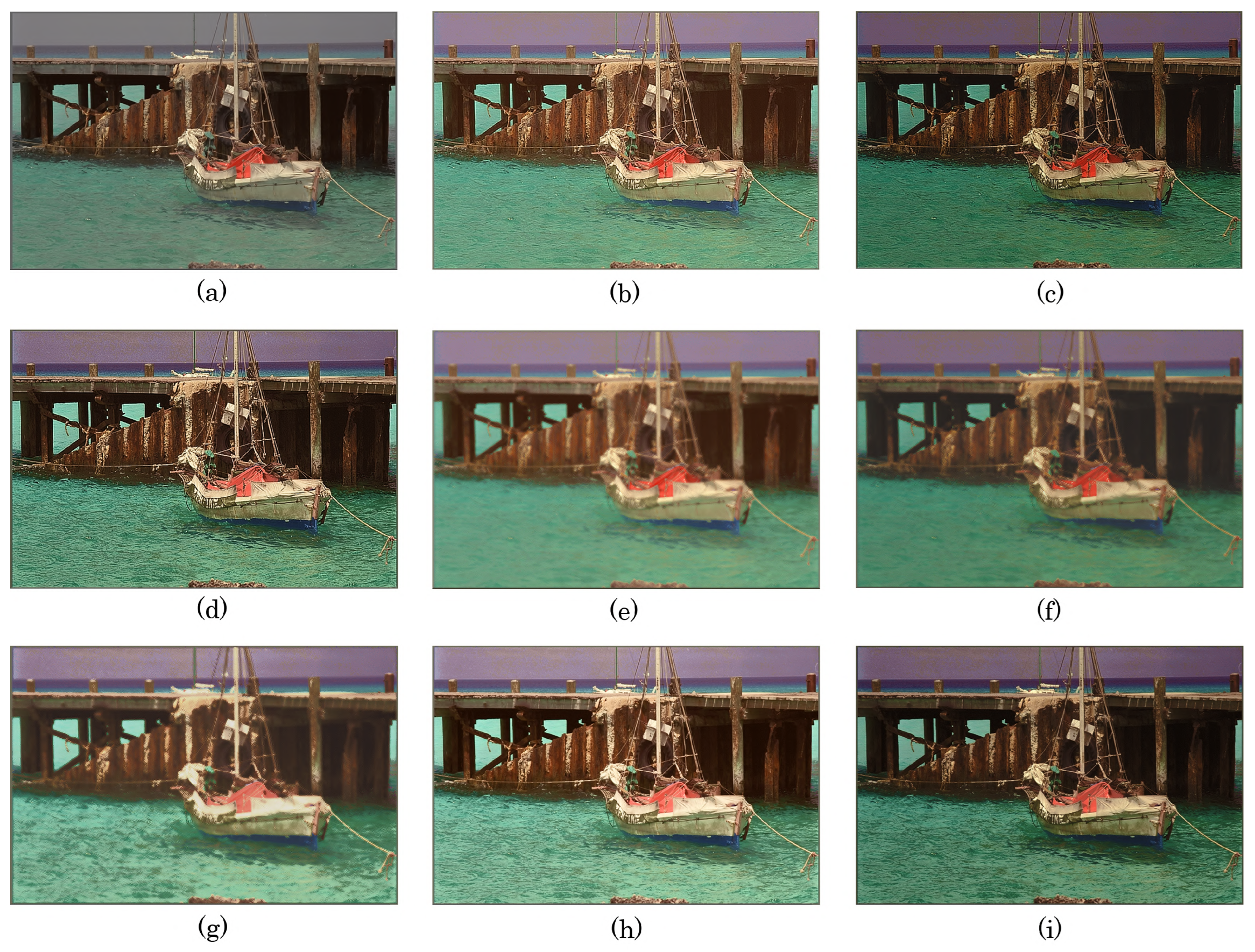
4.2. Visual and Quantitative Evaluation

First, we visually evaluated the output images with brightness control or saturation improvement. Figure 5 and Figure 6 shows the raw image and output images derived with the proposed method and previous methods [1,12]. In this experiment, we defined $I_{VSH}=I_{VSM}=$ 2, $I_{VI}=I_{VD}=I_{VC}=$ 30, and $I_S=$ 20. Figure 5b–f and Figure 6b–f demonstrate that the proposed method effectively executed a single brightness control from among the five types: sharpening and smoothing, increase and decrease, and CE. As can be seen in Figure 5g and Figure 6g, we can verify that our new method practically improved the saturation. In regard to the previous methods [1,12], they also enhanced the contrast as shown in Figure 5h,i and Figure 6h,i. These previous methods, however, cannot carry out other types of brightness controls and saturation improvement. Furthermore, Figure 5i and Figure 6i reveal that the previous method [1] caused hue distortion with the CE function.

Next, we quantitatively confirmed the availability of brightness control, saturation improvement, and hue preservation functions.

Table 2. Evaluations of brightness control, saturation improvement, and hue preservation.

		Brightness						Saturation		Hue
		Difference in Standard Deviations		Difference		RCE		Difference		Absolute Difference (degree)
		Saturation Improvement
		${\mathit{I}}_{\mathit{S}}$ = 0	${\mathit{I}}_{\mathit{S}}$ = 20	${\mathit{I}}_{\mathit{S}}$ = 20	${\mathit{I}}_{\mathit{S}}$ = 20	${\mathit{I}}_{\mathit{S}}$ = 0	${\mathit{I}}_{\mathit{S}}$ = 20	${\mathit{I}}_{\mathit{S}}$ = 0	${\mathit{I}}_{\mathit{S}}$ = 20	${\mathit{I}}_{\mathit{S}}$ = 0	${\mathit{I}}_{\mathit{S}}$ = 20
Sharpening	$I_{VSH}=$ 1	1.94	1.69	2.08	3.21	0.5076	0.5066	1.43	16.08	2.71	2.12
	$I_{VSH}=$ 2	3.52	3.12	4.44	6.07	0.5138	0.5123	0.53	14.86	4.28	3.87
Smoothing	$I_{VSM}=$ 1	−1.55	−1.96	3.06	5.57	0.4939	0.4923	1.68	16.87	3.66	2.80
	$I_{VSM}=$ 2	−4.04	−4.71	6.83	12.50	0.4842	0.4815	1.42	16.99	6.19	5.34
Brightness increase	$I_{VI}$ = 15	−1.05	−1.22	15.44	15.71	0.4959	0.4952	1.51	20.75	2.38	1.12
	$I_{VI}$ = 30	−2.61	−2.59	29.04	29.20	0.4898	0.4898	0.78	20.79	2.64	1.14
Brightness decrease	$I_{VD}$ = 15	−0.80	−0.84	−12.29	−11.91	0.4968	0.4967	0.06	12.02	2.86	2.28
	$I_{VD}$ = 30	−2.57	−2.57	−24.44	−23.82	0.4899	0.4899	−3.18	6.64	3.61	3.16
CE	$I_{VC}$ = 15	4.56	4.21	1.63	2.12	0.5179	0.5165	−1.26	14.32	2.43	1.39
	$I_{VC}$ = 30	8.39	7.99	3.27	3.56	0.5329	0.5313	−6.47	10.46	3.10	1.47
CE by prev. [12]	$I_{VC}$ = 15	5.64	-	−1.10	-	0.5221	-	−0.46	-	0.76	-
	$I_{VC}$ = 30	10.14	-	−0.55	-	0.5397	-	−0.24	-	0.87	-
CE by prev. [1]	$I_{VC}$ = 15	4.88	-	3.23	-	0.5191	-	0.59	-	16.72	-
	$I_{VC}$ = 30	7.27	-	9.40	-	0.5285	-	3.76	-	30.56	-

shows the mean value of each evaluation index for all the test images under different parameters. Note that $I_S=$ 0 means that the saturation is intact. In the case of the sharpening or smoothing function, the differences in standard deviations between the raw and output images increased or decreased. The brightness differences increased or decreased depending on the brightness increase or decrease function. With respect to the CE function, the RCE values exceeded 0.5 for the proposed and previous methods. The saturation differences increased in response to the saturation improvement function. In regard to the hue, the absolute differences were relatively small for the proposed method and previous method [12], while that of the previous method [1] was considerably large. From the aforementioned results, we verified that the proposed method has flexible functions for brightness and an improvement function for saturation without distorting the hue.

The proposed method has many advantages over the previous methods [1,12], but there still exists a constraint. To ensure reversibility, our new method requires the recovery information to be embedded as described in Section 3.1.3. This embedding process causes slight perceptual distortion and deteriorates the performance of each function.

4.3. Maximum Level of Each Process

Figure 7 shows the output images obtained with the maximum limit for each one of the functions. As shown in Figure 7b–g, the proposed method attained a wide range of control for each function. We can control the degree of effect of each function by regulating the parameters within the range from zero to the maximum. By using the previous methods [1,12], the contrast was enhanced to the maximum, as can be seen in Figure 7h,i. However, the method in [1] caused serious artifacts due to hue distortion, and the other method [12] could not guarantee reversibility.

We quantitatively analyzed the output images for all the test images in the case where the control level was at its maximum. Figure 8 shows the differences in standard deviations, brightness, RCE, and saturation. It is clear that the effect of each function with the maximum limit was much larger than that with the intermediate level shown in Table 2. Nonetheless, the effect depends on the features of the raw images, so it might not be fully effective for some images.

4.4. Reversibility

We confirmed the quality of the restored images obtained with each method.

Table 3. Quality of restored images.

		PSNR (dB)	SSIM	CIEDE2000
Sharpening	$I_{VSH}=$ 2	$+\infty$	1.0000	0.0000
Smoothing	$I_{VSM}=$ 2
Brightness increase	$I_{VI}=$ 30
Brightness decrease	$I_{VD}=$ 30
CE	$I_{VC}=$ 30
Saturation improvement	$I_S=$ 20
CE by prev. [12]	$I_{VC}=$ 30	59.16	0.9992	0.1001
CE by prev. [1]	$I_{VC}=$ 30	$+\infty$	1.0000	0.0000

shows the mean values of PSNR, SSIM, and CIEDE2000. We evaluated the image quality under $I_{VSH}=I_{VSM}=$ 2, $I_{VI}=I_{VD}=I_{VC}=$ 30, and $I_S=$ 20. As shown in this table, the proposed method and previous method [1] ensured perfect reversibility for all the test images. In comparison, the previous method [12] could never reconstruct the raw images completely, while the recovered images had a high image quality.

4.5. Effectiveness of Embedding Process

We compared the amount of recovery information with the hiding capacity. The previous methods [1,12] with the CE function used the RDH-based HS method [1] to enhance the contrast and embed the recovery information simultaneously. The proposed method also uses the RDH-based HS method for the CE function. If the amount of recovery information for CE exceeds the hiding capacity, then the residual information will be embedded later with the other recovery information in the proposed method. The recovery information for the other functions and the above residual information for CE were embedded using the PEE-HS method [19].

Figure 9 exhibits the hiding capacity, amount of the recovery information, and proportion of recovery information to the hiding capacity in the RDH-based HS and PEE-HS methods, where $I_{VSH}=I_{VSM}=$ 2, $I_{VI}=I_{VD}=I_{VC}=$ 30, and $I_S=$ 20. The proportion of recovery information to the hiding capacity is defined as

$$\begin{array}{c}\hfill Proportionofrecoveryinformationtohidingcapacity[\%]\\ \hfill & =\frac{Amountofrecoveryinformation}{Hidingcapacity}\times 100.\hfill \end{array}$$

(9)

In Figure 9c,f, all of the recovery information can be perfectly embedded when the index indicates a value less than 100%.

Figure 9a–c shows the results for the CE function using the HS method for each method. As can be seen in these figures, the previous methods [1,12] constantly embedded the entire recovery information. On the contrary, in the proposed method, the amount of recovery information was larger than the hiding capacity for several images. In such a case, the residual information would be embedded with the PEE-HS method as mentioned below.

Figure 9d–f exhibits the results for all the functions using the PEE-HS method in our new method. With respect to the CE function, the above residual information and the other essential recovery information were embedded in this process. In the other functions, all of the recovery information was embedded at once. According to these figures, it is clear that the proposed method could perfectly embed all of the recovery information in any function. Note that we calculated the hiding capacity under the condition that the PEE-HS method was carried out with a single repetition to ensure a sufficient capacity. The number of processing times was variable, depending on the amount of recovery information to be embedded.

4.6. Discussion on Coregulation

Here, we discuss coregulation, where multiple functions are simultaneously applied to a single image. We assumed that two types of brightness controls and saturation improvement were used. Figure 10 shows the output images under the condition where three functions were applied. One of the three functions was always saturation improvement. There existed eight combinations from which to choose two types of brightness controls: sharpening and brightness increase (Figure 10b), sharpening and brightness decrease (Figure 10c), sharpening and CE (Figure 10d), smoothing and brightness increase (Figure 10e), smoothing and brightness decrease (Figure 10f), smoothing and CE (Figure 10g), brightness increase and CE (Figure 10h), and brightness decrease and CE (Figure 10i). Note that we defined $I_{VSH}=I_{VSM}=$ 2, $I_{VI}=I_{VD}=I_{VC}=$ 30, and $I_S=$ 20 in this experiment. Here, the controllable range of each function depended on the features of the raw images. Thus, the above parameter values would not be adapted to any images. Through this experiment, we confirmed the effectiveness of coregulation with the proposed method. Note that if the output image would still have the residual capacity, then we could apply another function to the image. The discussion of this matter is our future work.

5. Conclusions

We proposed a novel image processing method for color images to reversibly control multiple functions. In particular, the proposed method attained not only CE but also sharpening and smoothing, brightness increase and decrease, and saturation improvements. This method has three main advantages. First, we verified that one or two types of functions can be used from among five brightness controls: sharpening and smoothing, brightness increase and decrease, and CE. Second, the regulations for the brightness and saturation can be executed independently. Specifically, the regulations never interfere with one another. Finally, full reversibility is ensured by embedding the recovery information so the raw images can be retrieved from the output images.

The experimental results demonstrated the availability of the proposed method from the standpoints of image quality and reversibility. We first confirmed the effect of each function visually and quantitatively. The proposed method flexibly controlled the brightness and improved the saturation without hue distortion. Next, we explored the maximum limit of each function. It was verified that this method has a wide range of control for each function. With respect to reversibility, the proposed method perfectly reconstructed the raw images in any case. For the embedding process, we compared the amount of recovery information with the hiding capacity. It was proven that the proposed method perfectly embedded all of the recovery information. We finally verified the performance of coregulation. Our method could effectively apply three functions, namely two types of brightness controls and saturation improvement, to a single image. Through our experiments, it is clear that the proposed method achieved multiple functions for brightness and saturation with full reversibility.

As described above, our new method has unique advantages over the previous methods. However, there still exists a constraint: the proposed method ensures reversibility for specific functions only. As one solution to tackle this matter, we will investigate flexible control for the hue component. Additionally, we aim to make the combination of multiple functions for a single image free so as to achieve more flexible processing.

References

1. Wu, H.-T.; Dugelay, J.-L.; Shi, Y.-Q. Reversible image data hiding with contrast enhancement. IEEE Signal Process. Lett. 2015, 22, 81–85. [Google Scholar]
2. Jafar, I.F.; Darabkh, K.A.; Saifan, R.R. SARDH: A novel sharpening-aware reversible data hiding algorithm. J. Vis. Commun. Image Represent. 2016, 39, 239–252. [Google Scholar]
3. Zhang, T.; Hou, T.; Weng, S.; Zou, F.; Zhang, H.; Chang, C.-C. Adaptive reversible data hiding with contrast enhancement based on multi-histogram modification. IEEE Trans. Circuits Syst. Video Technol. 2022, 32, 5041–5054. [Google Scholar]
4. Wu, H.-T.; Tang, S.; Huang, J.; Shi, Y.-Q. A novel reversible data hiding method with image contrast enhancement. Signal Process. Image Commun. 2018, 62, 64–73. [Google Scholar] [CrossRef]
5. Wu, H.-T.; Mai, W.; Meng, S.; Cheung, Y.-M.; Tang, S. Reversible data hiding with image contrast enhancement based on two-dimensional histogram modification. IEEE Access 2019, 7, 83332–83342. [Google Scholar]
6. Wu, H.-T.; Huang, J.; Shi, Y.-Q. A reversible data hiding method with contrast enhancement for medical images. J. Vis. Commun. Image Represent. 2015, 31, 146–153. [Google Scholar] [CrossRef]
7. Gao, G.; Wan, X.; Yao, S.; Cui, Z.; Zhou, C.; Sun, X. Reversible data hiding with contrast enhancement and tamper localization for medical images. Inf. Sci. 2017, 385–386, 250–265. [Google Scholar]
8. Yang, Y.; Zhang, W.; Liang, D.; Yu, N. A ROI-based high capacity reversible data hiding scheme with contrast enhancement for medical images. Multimed. Tools Appl. 2018, 77, 18043–18065. [Google Scholar] [CrossRef]
9. Kim, S.; Lussi, R.; Qu, X.; Kim, H.J. Automatic contrast enhancement using reversible data hiding. In Proceedings of the IEEE International Workshop on Information Forensics and Security, Rome, Italy, 16–19 November 2015; pp. 1–5. [Google Scholar]
10. Kim, S.; Lussi, R.; Qu, X.; Huang, F.; Kim, H.J. Reversible data hiding with automatic brightness preserving contrast enhancement. IEEE Trans. Circuits Syst. Video Technol. 2019, 29, 2271–2284. [Google Scholar] [CrossRef]
11. Wu, H.-T.; Cao, X.; Jia, R.; Cheung, Y.-M. Reversible data hiding with brightness preserving contrast enhancement by two-dimensional histogram modification. IEEE Trans. Circuits Syst. Video Technol. 2022, 32, 7605–7617. [Google Scholar] [CrossRef]
12. Wu, H.-T.; Wu, Y.; Guan, Z.; Cheung, Y.-M. Lossless Contrast Enhancement of Color Images with Reversible Data Hiding. Entropy 2019, 21, 910. [Google Scholar] [CrossRef]
13. Sugimoto, Y.; Imaizumi, S. An Extension of Reversible Image Enhancement Processing for Saturation and Brightness Contrast. J. Imaging 2022, 8, 27. [Google Scholar] [PubMed]
14. Kumar, C.; Singh, A.K.; Kumar, P. A recent survey on image watermarking techniques and its application in e-governance. Multimed. Tools Appl. 2018, 77, 3597–3622. [Google Scholar] [CrossRef]
15. Shi, Y.-Q.; Li, X.; Zhang, X.; Wu, H.-T.; Ma, B. Reversible data hiding: Advances in the past two decades. IEEE Access 2016, 4, 3210–3237. [Google Scholar] [CrossRef]
16. Smith, A.R. Color gamut transform pairs. Comput. Graph. 1978, 12, 12–19. [Google Scholar] [CrossRef]
17. Hamachi, T.; Tanabe, H.; Yamawaki, A. Development of a Generic RGB to HSV Hardware. In Proceedings of the 1st International Conference on Industrial Applications Engineering 2013, Fukuoka, Japan, 27–28 March 2013; pp. 169–173. [Google Scholar]
18. Zhou, Y.; Chen, Z.; Huang, X. A system-on-chip FPGA design for real-time traffic signal recognition system. In Proceedings of the 2016 IEEE International Symposium on Circuits and Systems (ISCAS), Montreal, QC, Canada, 22–25 May 2016; pp. 1778–1781. [Google Scholar]
19. Thodi, D.M.; Rodriguez, J.J. Expansion Embedding Techniques for Reversible Watermarking. IEEE Trans. Image Process. 2007, 16, 721–730. [Google Scholar] [CrossRef] [PubMed]
20. Howard, P.G.; Kossentini, F.; Martins, B.; Forchhammer, S.; Rucklidge, W.J. The emerging JBIG2 standard. IEEE Trans. Circuits Syst. Video Technol. 1998, 8, 838–848. [Google Scholar]
21. Kodak Lossless True Color Image Suite. Available online: http://www.r0k.us/graphics/kodak/ (accessed on 14 October 2022).
22. The USC-SIPI Image Database. Available online: https://sipi.usc.edu/database/ (accessed on 14 October 2022).
23. McMaster Dataset. Available online: https://www4.comp.polyu.edu.hk/~cslzhang/CDM_Dataset.htm (accessed on 14 October 2022).
24. IHC Evaluation Resources. Available online: https://www.ieice.org/iss/emm/ihc/ (accessed on 14 October 2022).
25. ITE Evaluation Resources. Available online: https://www.ite.or.jp/content/chart/uhdtv/ (accessed on 14 October 2022).
26. Gao, M.Z.; Wu, Z.G.; Wang, L. Comprehensive evaluation for HE based contrast enhancement techniques. Adv. Intell. Syst. Appl. 2013, 2, 331–338. [Google Scholar]
27. Wang, Z.; Bovik, A.C.; Sheikh, H.R.; Simoncelli, E.P. Image quality assessment: From error visibility to structural similarity. IEEE Trans. Image Process. 2004, 13, 600–612. [Google Scholar] [CrossRef] [PubMed] [Green Version]
28. Sharma, G.; Wu, W.; Dalal, E.N. The CIEDE2000 color-difference formula: Implementation notes, supplementary test data, and mathematical observations. Color Res. 2005, 30, 21–30. [Google Scholar]
Figure 1. Block diagram of our previous method [13].
Applsci 13 02297 g001
Figure 2. Block diagrams of proposed method. (a) Image processing. (b) Raw image recovery.
Applsci 13 02297 g002
Figure 3. Sharpening and smoothing using M a x . (a) Region segmentation. (b) Target and reference points.
Applsci 13 02297 g003
Figure 4. Histogram transition of M a x and M i n for brightness increase function. (a) Raw histograms and integrated histogram of M a x and M i n (b) In case the reference bin is empty. (c) In case the reference bin is not empty. (d) Separation into M a x and M i n .
Applsci 13 02297 g004
Figure 5. Raw image and output images from proposed and previous methods [1,12] (kodim11). (a) Raw image. (b) Sharpening ( I V S H = 2). (c) Smoothing ( I V S M = 2). (d) Brightness increase ( I V I = 30). (e) Brightness decrease ( I V D = 30). (f) CE ( I V C = 30). (g) Saturation improvement ( I S = 20). (h) CE under previous method [12] ( I V C = 30). (i) CE under previous method [1] ( I V C = 30).
Applsci 13 02297 g005
Figure 6. Raw image and output images through proposed and previous methods [1,12] (Ship). (a) Raw image. (b) Sharpening ( I V S H = 2). (c) Smoothing ( I V S M = 2). (d) Brightness increase ( I V I = 30). (e) Brightness decrease ( I V D = 30). (f) CE ( I V C = 30). (g) Saturation improvement ( I S = 20). (h) CE under previous method [12] ( I V C = 30). (i) CE under previous method [1] ( I V C = 30).
Applsci 13 02297 g006
Figure 7. Maximum level of each brightness control and saturation improvement (kodim11). (a) Raw image. (b) Sharpening ( I V S H = 3). (c) Smoothing ( I V S M = 4). (d) Brightness increase ( I V I = 140). (e) Brightness decrease ( I V D = 139). (f) CE ( I V C = 59). (g) Saturation improvement ( I S = 182). (h) CE under previous method [12] ( I V C = 50). (i) CE under previous method [1] ( I V C = 64).
Applsci 13 02297 g007
Figure 8. Maximum level of each evaluation index. (a) Difference in standard deviations. (b) Brightness difference. (c) RCE for proposed and previous methods [1,12]. (d) Saturation difference.
Applsci 13 02297 g008
Figure 9. Performance of HS and PEE-HS methods ( I V S H = I V S M = 2, I V I = I V D = I V C = 30, and I S = 20). (a) Hiding capacity (HS) for proposed and previous methods [1,12]. (b) Amount of recovery information (HS) for proposed and previous methods [1,12]. (c) Proportion of recovery information to hiding capacity (HS) for proposed and previous methods [1,12]. (d) Hiding capacity (PEE-HS). (e) Amount of recovery information (PEE-HS). (f) Proportion of recovery information to hiding capacity (PEE-HS).
Applsci 13 02297 g009
Figure 10. Raw image and output images under proposed method with two types of brightness controls and saturation improvement (kodim11, I S = 20). (a) Raw image. (b) Sharpening and brightness increase ( I V S H = 2 and I V I = 30). (c) Sharpening and brightness decrease ( I V S H = 2 and I V D = 30). (d) Sharpening and CE ( I V S H = 2 and I V C = 30). (e) Smoothing and brightness increase ( I V S M = 2 and I V I = 30). (f) Smoothing and brightness decrease ( I V S M = 2 and I V D = 30). (g) Smoothing and CE ( I V S M = 2 and I V C = 30). (h) Brightness increase and CE ( I V I = 30 and I V C = 30). (i) Brightness decrease and CE ( I V D = 30 and I V C = 30).
Applsci 13 02297 g010